Feb 3, 2015 - a merely âmodalâ interpretation by requiring the brackets to take values in Z2 (1 = possible, 0 = impossible). But the usual QM brackets ãÏ|Ïã ...
arXiv:1502.01048v1 [quant-ph] 3 Feb 2015
On classical finite probability theory as a quantum probability calculus David Ellerman Department of Philosophy U. of California/Riverside February 5, 2015 Abstract This paper shows how the classical finite probability theory (with equiprobable outcomes) can be reinterpreted and recast as the quantum probability calculus of a pedagogical or ”toy” model of quantum mechanics over sets (QM/sets). There have been four previous attempts to develop a quantum-like model with the base field of C replaced by Z2 , but they are all forced into a merely ”modal” interpretation by requiring the brackets to take values in Z2 (1 = possible, 0 = impossible). But the usual QM brackets hψ|ϕi give the ”overlap” between states ψ and ϕ, so for sets S, T ⊆ U , the natural definition is hS|T i = |S ∩ T |. This allows QM/sets to be developed with a full probability calculus that turns out to be the perfectly classical Laplace-Boole finite probability theory. The point is not to clarify finite probability theory but to elucidate quantum mechanics itself by seeing some of its quantum features (e.g., two-slit experiment) in a classical setting.
Contents 1 Introduction
2
2 Laplace-Boole probability theory
2
3 Recasting finite probability theory as a quantum probability calculus 3.1 Vector spaces over Z2 . . . . . . . . . . . . . . . . . . . . . . . . . . . . . 3.2 The brackets . . . . . . . . . . . . . . . . . . . . . . . . . . . . . . . . . . 3.3 Ket-bra resolution . . . . . . . . . . . . . . . . . . . . . . . . . . . . . . . 3.4 The norm . . . . . . . . . . . . . . . . . . . . . . . . . . . . . . . . . . . . 3.5 Numerical attributes and linear operators . . . . . . . . . . . . . . . . . . 3.6 Completeness and orthogonality of projection operators . . . . . . . . . . 3.7 The Born Rule for measurement in QM and QM/sets . . . . . . . . . . . 3.8 Summary of QM/sets and QM . . . . . . . . . . . . . . . . . . . . . . . .
. . . . . . . .
. . . . . . . .
. . . . . . . .
. . . . . . . .
. . . . . . . .
. . . . . . . .
3 3 4 4 5 5 6 7 8
4 Measurement in QM/sets 4.1 Measurement, Partitions, and Distinctions . . . 4.2 Example of a nondegenerate measurement . . . 4.3 Example of a degenerate measurement . . . . . 4.4 Measurement using density matrices . . . . . . 4.5 Quantum dynamics and the two-slit experiment
. . . . .
. . . . .
. . . . .
. . . . .
. . . . .
. . . . .
8 8 10 11 12 15
5 Further steps
. . . . . . . . . . . . . . . . . . . . . . . . . . . . in QM/sets
. . . . .
. . . . .
. . . . .
. . . . .
. . . . .
. . . . .
. . . . .
. . . . .
18 1
1
Introduction
This paper develops a pedagogical or ”toy” model of quantum mechanics over sets (QM/sets) where the quantum probability calculus is the ordinary Laplace-Boole finite logical probability theory ([15], [2]) and where the usual vector spaces over C for QM are replaced with vector spaces over Z2 in QM/sets. Quantum mechanics over sets is a bare-bones ”logical” (e.g., non-physical1 ) version of QM with appropriate versions of spectral decomposition, the Dirac brackets, ket-bra resolution, the norm, observable-attributes, and the Born rule all in the simple classical setting of sets, but that nevertheless provides models of characteristically quantum results (e.g., a QM/sets version of the double-slit experiment). In that manner, QM/sets can serve not only as a pedagogical (or ”toy”) model of QM but perhaps as an engine to better elucidate QM itself by representing the quantum features in a simple classical setting. There have been at least four previous attempts at developing a version of QM over sets, i.e., where the base field of C is replaced by Z2 ([18], [13], [19], and [1]). All these attempts use the aspect of full QM that the brackets and the observables take their values in the base field. When the base field is Z2 , then the models do ”not make use of the idea of probability”[18, p. 919] and have instead only a modal interpretation (1 = possibility and 0 = impossibility). The model of QM over sets developed here is based on a different understanding of the relation between the pedagogical model and full QM. Instead of trying to mimic QM (replacing C with Z2 ), the idea is that QM/sets can perfectly well have the brackets and observables take values outside the base field of Z2 (e.g., use real-valued observables = real-valued random variables in classical finite probability theory) and even defining a more primitive version of ”eigenvectors” and ”eigenvalues” that are not (in general) the eigenvectors and eigenvalues of linear operators on the vector space over Z2 . The transitioning from QM/sets to full QM is then seen not as going from one model to another model of a set of axioms (e.g., as in [1]) but as a process of ”internalization” allowed by increasing the base field from Z2 to C. The increased power of C (e.g., algebraic completeness) then allows the primitive ”eigenvectors” and ”eigenvalues” of QM/sets to be ”internalized” as true eigenvectors and eigenvalues of (Hermitian) linear operators on vector spaces over C and the brackets can then also be ”internalized” as a bilinear inner product taking values in the base field C. Hence under this approach (and in contrast to the four previous approaches), the ”taking values in the base field” is seen only as an aspect of full QM over C and not as a necessary aspect of a pedagogical proto-QM model such as QM/sets with the base field of Z2 .
2
Laplace-Boole probability theory
Since our purpose is conceptual rather than mathematical, we will stick to the simplest case of finite probability theory with a finite sample space U = {u1 , ..., un } of n equiprobable outcomes and to finite dimensional QM.2 The events are the subsets S ⊆ U , and the probability of an event S |S| . Given that a conditioning event occurring in a trial is the ratio of the cardinalities: Pr (S) = |U| ∩S) |T ∩S| S ⊆ U occurs, the conditional probability that T ⊆ U occurs is: Pr(T |S) = Pr(T Pr(S) = |S| . The ordinary probability Pr (T ) of an event T can be taken as the conditional probability with U as the conditioning event so all probabilities can be seen as conditional probabilities. Given a (real-valued) random variable, i.e., a numerical attribute f : U → R on the elements of U , the probability of observing a value r given an event S is the conditional probability of the event f −1 (r) given S:
Pr (r|S) =
|f −1 (r)∩S | |S|
.
1 In full QM, the DeBroglie relations connect mathematical notions such as frequency and wave-length to physical notions such as energy and momentum. QM/sets is ”non-physical” in the sense that it is a sets-version of the pure mathematical framework of (finite-dimensional) QM without those direct physical connections. 2 The mathematics can be generalized to the case where each point u in the sample space has a probability p but i i the simpler case of equiprobable points serves our conceptual purposes.
2
That is all the probability theory we will need here. Our task is to show how the mathematics of finite probability theory can be recast using the mathematical notions of quantum mechanics with the base field of Z2 is substituted, mutatis mutandis, for the complex numbers C.
3
Recasting finite probability theory as a quantum probability calculus
3.1
Vector spaces over Z2
To show how classical Laplace-Boole finite probability theory can be recast as a quantum probability calculus, we use finite dimensional vector spaces over Z2 .3 The power set ℘ (U ) of U = {u1 , ..., un } is a vector space over Z2 = {0, 1}, isomorphic to Zn2 , where the vector addition S + T is the symmetric difference (or inequivalence) of subsets. That is, for S, T ⊆ U , S + T = (S − T ) ∪ (T − S) = S ∪ T − S ∩ T . The U -basis in ℘ (U ) is the set of singletons {uP 1 } , {u2 } , ..., {un }, i.e., the set {{u}}u∈U . A vector by its Z2 -valued S ∈ ℘ (U ) is specified in the U -basis as S = u∈S {u} and it is characterized P characteristic function χS : U → Z2 ⊆ R of coefficients since S = u∈U χS (u) P{u}. Similarly, a vector v in Cn is specified in terms of an orthonormal basis {|vi i} as v = i ci |vi i and is characterized by a C-valued function h |vi : {vi } → C assigning a complex amplitude hvi |vi = ci to each basis vector |vi i. One of the key pieces of mathematical machinery in QM, namely the inner product, does not exist in vector spaces over finite fields but brackets can still be defined starting with h{u} |U Si = χS (u) (see below) and a norm can be defined to play a similar role in the probability calculus of QM/sets. Seeing ℘ (U ) as the abstract vector space Zn2 allows different bases in which the vectors can be expressed (as well as the basis-free notion of a vector as a ”ket”). Hence the quantum probability calculus developed here can be seen as a ”non-commutative” generalization of the classical LaplaceBoole finite probability theory where a different basis corresponds to a different equicardinal sample space U ′ = {u′1 , ..., u′n }. Consider the simple case of U = {a, b, c} where the U -basis is {a}, {b}, and {c}. The three subsets {a, b}, {b, c}, and {a, b, c} also form a basis since: {b, c} + {a, b, c} = {a}; {b, c} + {a, b} + {a, b, c} = {b}; and {a, b} + {a, b, c} = {c}. These new basis vectors could be considered as the basis-singletons in another equicardinal universe U ′ = {a′ , b′ , c′ } where {a′ }, {b′ }, and {c′ } refer to the same abstract vector as {a, b}, {b, c}, and {a, b, c} respectively. In the following ket table, each row is an abstract vector of Z32 expressed in the U -basis, the ′ U -basis, and a U ′′ -basis. U = {a, b, c} {a, b, c} {a, b} {b, c} {a, c} {a} {b} {c} ∅ 3 We
U ′ = {a′ , b′ , c′ } {c′ } {a′ } {b′ } {a′ , b′ } {b′ , c′ } {a′ , b′ , c′ } {a′ , c′ } ∅
U ′′ = {a′′ , b′′ , c′′ } {a′′ , b′′ , c′′ } {b′′ } {b′′ , c′′ } {c′′ } {a′′ } {a′′ , b′′ } {a′′ , c′′ } ∅
are assuming some basic familarity with the mathematics of finite dimensional QM.
3
Vector space isomorphism: Z32 ∼ = ℘ (U ) ∼ = ℘ (U ′ ) ∼ = ℘ (U ′′ ) where row = ket. In the Dirac notation [4], the ket |{a, c}i represents the abstract vector that is represented in the U -basis as {a, c}. A row of the ket table gives the different representations of the same ket in the different bases, e.g., |{a, c}i = |{a′ , b′ }i = |{c′′ }i.
3.2
The brackets
p In a Hilbert space, the inner product is used to define the brackets hvi |vi and the norm |v| = hv|vi. In a vector space over Z2 , the Dirac notation can still be used to define the brackets and norm even though there is no inner product. For a singleton basis vector {u} ⊆ U , the bra h{u}|U : ℘ (U ) → R is defined by the bracket : � 1 if u ∈ S h{u} |U Si = = |{u} ∩ S| = χS (u). 0 if u ∈ /S Note that the bra and the bracket is defined in terms of the U -basis and that is indicated by the U -subscript on the bra portion of the bracket. Then for ui , uj ∈ U , h{ui } |U {uj }i = χ{uj } (ui ) = χ{ui } (uj ) = δij (the Kronecker delta function) which is the QM/sets-version of hvi |vj i = δij for an orthonormal basis {|vi i} of Cn . The bracket linearly extends in the reals to any two vectors T, S ∈ ℘ (U ):4 hT |U Si = |T ∩ S|. This is the QM/sets-version of the Dirac brackets in the mathematics of QM. For more motivation, consider an orthonormal basis set {|vi i}i=1,...,n in an n-dimensional P Hilbert space V and the association {ui } ↔ |vi i for i = 1, ..., n. Given two subsets T, S ⊆ U , T = ui ∈T {ui } P corresponds to the unnormalized ψT = ui ∈T |vi i and similarly for ψS . Then their inner product (defined using the {|vi i}i=1,...,n basis) in V is hψT |ψS i = |T ∩ S| = hT |U Si. In both cases, the bracket gives a measure of the overlap or indistinctness of the two vectors.5
3.3
Ket-bra resolution
The ket-bra |{u}i h{u}|U is defined as the one-dimensional projection operator: |{u}i h{u}|U = {u} ∩ () : ℘ (U ) → ℘ (U ) and the ket-bra identity holds as usual: P P u∈U ({u} ∩ ()) = I : ℘ (U ) → ℘ (U ) u∈U |{u}i h{u}|U =
where the summation is the symmetric difference of sets in ℘ (U ) and I is the identity map [as a linear operator on ℘ (U )]. The overlap hT |U Si can be resolved using the ket-bra identity in the same basis: 4 Here hT | Si = |T ∩ S| takes values outside the base field of Z just like, say, the Hamming distance function 2 U dH (T, S) = |T + S| on vector spaces over Z2 in coding theory. [16] Thus the bra hS|U is not to be confused with the dual functional χS : ℘ (U ) → Z2 that does take values in the base field. The brackets taking values in the base field is a consequence of the base field being strengthened to C. It is not a necessary feature of a quantum probability calculus as we see in QM/sets. 5 Indeed in QM/sets, the brackets hT | Si = |T ∩ S| for T, T ′ , S ⊆ U should be thought of only as a measure of the U overlap since they are not even linear, e.g., hT + T ′ |U Si = 6 hT |U Si + hT ′ |U Si whenever T ∩ T ′ 6= ∅. Only as the base field Z2 is increased to C (or R) do the brackets ’fall into place’ as a bilinear inner product. QM/sets is not ’supposed’ to have completely the same mathematical structure as QM only with Z2 replacing C. QM/sets is a proto-QM where things only ’fall into place’ and are ’internalized’ as the transition is made from Z2 to C as the base field.
4
hT |U Si =
P
u
hT |U {u}i h{u} |U Si.
Similarly a ket |Si for S ⊆ U can be resolved in the U -basis; P P P |Si = u∈U |{u}i h{u} |U Si = u∈U h{u} |U Si |{u}i = u∈U |{u} ∩ S| |{u}i
where a subset S ⊆ U is just expressed as the sum of the singletons {u} ⊆ S. That is ket-bra resolution in QM/sets. The ket |Si is the same as the ket |S ′ i for some subset S ′ ⊆ U ′ in another U ′ -basis, but when the bra h{u}|U is applied to the ket |Si = |S ′ i, then it is the subset S ⊆ U , not S ′ ⊆ U ′ , that comes outside the ket symbol |i in h{u} |U Si = |{u} ∩ S|.6
3.4
The norm
The U -norm kSkU : ℘ (U ) → R is defined, as usual, as the square root of the bracket:7 p p p kSkU = hS|U Si = |S ∩ S| = |S| p for S ∈ ℘ (U ) which is the QM/sets-version of the norm |ψ| = hψ|ψi in ordinary QM. Note that √a ket has to be expressed in the U -basis to apply the U -norm definition so, for example, k{a′ }kU = 2 since |{a′ }i = |{a, b}i.
3.5
Numerical attributes and linear operators
In classical physics, the observables are numerical attributes, e.g., the assignment of a position and momentum to particles in phase space. One of the differences between classical and quantum physics is the replacement of these observable numerical attributes by linear operators associated with the observables where the values of the observables appear as eigenvalues of the operators. But this difference may be smaller than it would seem at first since a numerical attribute f : U → R can be recast into an operator-like format in QM/sets, and there is even a QM/sets-analogue of spectral decomposition. An observable, i.e., a Hermitian operator, on a Hilbert space V has a home basis set of orthonormal eigenvectors. In a similar manner, a real-valued attribute f : U → R defined on U has the U -basis as its ”home basis set.” The connection between the numerical attributes f : U → R of QM/sets and the Hermitian operators of full QM can be established by seeing the function f as being like an ”operator” f ↾ () on ℘ (U ) in that it is used to define a sets-version of an ”eigenvalue” equation [where f ↾ S is the restriction of f to S ∈ ℘ (U )]. For any subset S ∈ ℘ (U ), the definition of the equation is: f ↾ S = rS holds iff f is constant on the subset S with the value r. This is the QM/sets-version of an eigenvalue equation for numerical attributes f : U → R. Whenever S satisfies f ↾ S = rS for some r, then S is said to be an eigenvector in the vector space ℘ (U ) of the numerical attribute f : U → R, and � r ∈ R is the associated eigenvalue. Each eigenvalue r determines as usual an eigenspace ℘ f −1 (r) of its eigenvectors which is a subspace of the vector space ℘ (U ). The whole space ℘� (U ) can be expressed as usual as the direct sum of the eigenspaces: ℘ (U ) = L −1 (r) . Moreover, for distinct eigenvalues r 6= r′ , any corresponding eigenvectors S ∈ r∈f (U) ℘� f � ℘ f −1 (r) and T ∈ ℘ f −1 (r′ ) are orthogonal in the sense that hT |U Si = 0. In general, for vectors S, T ∈ ℘ (U ), orthogonality means zero overlap, i.e., disjointness. 6 The term ”{u} ∩ S ′ ” is not even defined since it is the intersection of subsets {u} ⊆ U and S ′ ⊆ U ′ of two different universe sets U and U ′ . 7 We use the double-line notation kSk U for the U -norm of a set to distinguish it from the single-line notation |S| for the cardinality of a set, whereas the customary absolute value notation for the norm of a vector v in ordinary QM p is |v| = hv|vi. The context should suffice to distinguish |S| from |v|.
5
The characteristic function χS : U → R for S ⊆ U has the eigenvalues of 0 and 1 so it is a numerical attribute that can be ”internalized” as a linear operator S ∩ () : ℘ (U ) → ℘ (U ). Hence in this case, the ”eigenvalue equation” f ↾ T = rT for f = χS becomes an actual eigenvalue equation S ∩ T = rT for a linear8 operator S ∩ () with the resulting eigenvalues of 1 and 0, and with the resulting eigenspaces ℘ (S) and ℘ (S c ) (where S c is the complement of S) agreeing with those ”eigenvalues” and ”eigenspaces” defined above for an arbitrary numerical attribute f : U → R. The characteristic attributes χS : U → R are characterized by the property that their value-wise product, i.e., (χS • χS ) (u) = χS (u) χS (u), is equal to the attribute value χS (u), and that is reflected in the idempotency of the corresponding operators: S∩()
S∩()
S∩()
℘ (U ) −→ ℘ (U ) −→ ℘ (U ) = ℘ (U ) −→ ℘ (U ). Thus the operators S ∩ () corresponding to the characteristic attributes χS are projection operators.9 The (maximal) f −1 (r) for f , with r in the image or spectrum f (U ) ⊆ R, span the P eigenvectors −1 set U , i.e., U = r∈f (U) f (r). Hence the attribute f : U → R has a spectral decomposition in terms of its (projection-defining) characteristic functions: P f = r∈f (U) rχf −1 (r) : U → R Spectral decomposition of set attribute f : U → R P which is the QM/sets-version of the spectral decomposition L = λ λPλ of a Hermitian operator L in terms of the projection operators Pλ for its eigenvalues λ.
3.6
Completeness and orthogonality of projection operators
For any vector S ∈ ℘ (U ), the operator S ∩ () : ℘ (U ) → ℘ (U ) is the linear projection operator to the subspace ℘ (S) ⊆ ℘ (U ). The usual completeness and orthogonality conditions on projection operators Pλ to the eigenspaces of an observable-operator have QM/sets-versions for numerical attributes f : U → R: P 1. completeness: λ Pλ = I : V → V in QM has the QM/sets-version: P −1 (r) ∩ () = I : ℘ (U ) → ℘ (U ), and rf Pµ
0
P
λ 2. orthogonality: for λ 6= µ, V −→ V −→ V = V −→ V (where 0 is the zero operator) has the ′ QM/sets-version: for r 6= r ,
℘ (U )
f −1 (r ′ )∩()
−→
℘ (U )
f −1 (r)∩()
−→
0
℘ (U ) = ℘ (U ) −→ ℘ (U ).
Note that in spite of the lack of an inner product, the orthogonality of projection operators S ∩ () is perfectly well-defined in QM/sets where it boils down to the disjointness of subsets, i.e., the cardinality of subsets’ overlap (instead of their inner product) being 0. 8 It should be noted that the projection operator S ∩ () : ℘ (U ) → ℘ (U ) is not only idempotent but linear, i.e., (S ∩ T1 ) + (S ∩ T2 ) = S ∩ (T1 + T2 ). Indeed, this is the distributive law when ℘ (U ) is interpreted as a Boolean ring with intersection as multiplication. 9 In order for general real-valued attributes to be internalized as linear operators, in the way that characteristic functions χS were internalized as projection operators S ∩ (), the base field would have to be strengthened to C and that would take us, mutatis mutandis, from the probability calculus of QM/sets to that of full QM.
6
3.7
The Born Rule for measurement in QM and QM/sets
An orthogonal decomposition of a finite set U is just a partition π = {B} of U since the blocks B, B ′ , ... are orthogonal (i.e., disjoint) and their sum is U . Given such an orthogonal decomposition of U , we have the: P kU k2U = B∈π kBk2U Pythagorean Theorem for orthogonal decompositions of sets. An old question is: ”why the squaring of amplitudes in the Born rule of QM?” A superposition state between certain definite orthogonal alternatives A and B, where the latter are represented by → − → − → − − → − → vectors A and B , is represented by the vector sum C = A + B . But what is the ”strength,” ”inten→ − → − → − sity,” or relative importance of the vectors A and B in the vector sum C ? That question requires a scalar measure of strength or magnitude or ”length” given by the norm kk does not
−
intensity.
→ The →
→ −
−
answer the question since A + B 6= C . But the Pythagorean Theorem shows that the norm
−
→ 2 −
→ 2
→ 2 − squared gives the scalar measure of ”intensity” that answers the question: A + B = C in vector spaces over Z2 or over C. And when the superposition state is reduced by a measurement, then the probability that the indefinite state will reduce to one of the definite alternatives is given by that relative scalar measure of the eigen-alternative’s ”strength” or ”intensity” in the indefinite state–and that is the Born Rule. In a slogan, Born is the off-spring of Pythagoras. Given an orthogonal basis {|vi i} in a finite dimensional Hilbert space and given the U -basis for the vector space ℘ (U ), the corresponding Pythagorean results for the basis sets are: |ψ|2 =
P hvi |ψi∗ hvi |ψi = i |hvi |ψi|2 and P 2 2 kSkU = u∈U h{u} |U Si .
P
i
Given an observable-operator in QM and a numerical attribute in QM/sets, the corresponding Pythagorean Theorems for the complete sets of orthogonal projection operators are: P 2 2 |ψ| = λ |Pλ (ψ)| and
P P 2 2 kSkU = r f −1 (r) ∩ S U = r f −1 (r) ∩ S = |S|. Normalizing gives:
|Pλ (ψ)|2 = 1 and |ψ|2 P |f −1 (r)∩S | P kf −1 (r)∩S k2U = r r |S| kSk2U
P
λ
=1
so the non-negative summands can be interpreted as probabilities–which is the Born rule in QM and in QM/sets.10 (ψ)|2 is the ”mysterious” quantum probability of getting λ in an L-measurement of ψ, Here |Pλ|ψ| 2 kf −1 (r)∩S k2U |f −1 (r)∩S | while = has the rather unmysterious interpretation in the pedagogical model, |S| kSk2U QM/sets, as the probability Pr (r|S) of the numerical attribute f : U → R having the eigenvalue r when ”measuring” S ∈ ℘ (U ). Thus the QM/sets-version of the Born Rule is the perfectly ordinary 10 Note that there is no notion of a normalized vector in a vector space over Z (another consequence of the lack of 2 an inner product). The normalization is, as it were, postponed to the probability algorithm which is computed in the reals. This ”external” probability algorithm is ”internalized” when Z2 is strengthened to C in going from QM/sets to full QM.
7
|f −1 (r)∩S | , that given S ⊆ U , a random Laplace-Boole rule for the conditional probability Pr (r|S) = |S| variable f : U → R takes the value r. In QM/sets, when the indefinite state S is being ”measured” using the observable f where the 2 kf −1 (r)∩S kU |f −1 (r)∩S | probability Pr (r|S) of getting the eigenvalue r is = , the ”damned quantum 2 |S| kSk U
jump” (Schr¨odinger) goes from S by the projection operator f −1 (r) ∩ () to the projected resultant � −1 −1 state f (r) ∩ S which is in the eigenspace ℘ f (r) for that eigenvalue r. The state resulting from the measurement represents a more-definite state f −1 (r) ∩ S that now has the definite f -value of r–so a second measurement would yield the same eigenvalue r with probability: � |f −1 (r)∩[f −1 (r)∩S ]| |f −1 (r)∩S | = |f −1 (r)∩S| = 1 Pr r|f −1 (r) ∩ S = |f −1 (r)∩S| � � and the same resulting vector f −1 (r) ∩ f −1 (r) ∩ S = f −1 (r) ∩ S using the idempotency of the projection operators. Hence the treatment of measurement in QM/sets is all analogous to the treatment of measurement in standard Dirac-von-Neumann QM.
3.8
Summary of QM/sets and QM
The QM/set-versions of the corresponding QM notions are summarized in the following table for the finite U -basis of the Z2 -vector space ℘ (U ) and for an orthonormal basis {|vi i} of a finite dimensional Hilbert space V . QM/sets over Z2 Projections: S ∩ () : ℘ (U ) → P ℘ (U ) Spectral Decomposition.: f = r rχf −1 (r) P −1 Completeness.: f (r) ∩ () = I� r �� � Orthog.: r 6= r′ , f −1 (r) ∩ () f −1 (r′ ) ∩ () = ∅ ∩ () Brackets:PhS|U T i = |S ∩ T | = P overlap of S, T ⊆ U = Ket-bra: u∈U |{u}i h{u}| u∈U ({u} ∩ ()) = I U P hS| Resolution: hS|p T i = U u pU {u}i h{u} |U T i Norm: kSkU = hS|U Si = |S| where S ⊆ U P 2 2 Basis Pythagoras: kSkU = u∈U h{u} |U Si = |S| P P h{u}|U Si2 1 =1 = u∈S |S| Normalized: u∈U kSk2 U
2
U Si Basis Born rule: Pr ({u} |S) = h{u}| kSk2U
2 P Attribute Pythagoras: kSk2U = r f −1 (r) ∩ S U P |f −1 (r)∩S | P kf −1 (r)∩S k2U = r =1 Normalized: r |S| kSk2U 2 −1 −1 kf (r)∩S kU |f (r)∩S | = Attribute Born rule: Pr(r|S) = |S| kSk2
Standard QM over C P :V →V P where P 2 = P LP= λ λPλ λ Pλ = I λ 6= µ, Pλ Pµ = 0 hψ|ϕi = Poverlap of ψ and ϕ i |v Pi i hvi | = I hψ|vi i hvi |ϕi hψ|ϕi = ip |ψ| = hψ|ψi P ∗ 2 |ψ| = i hvi |ψi hvi |ψi P hvi |ψi∗ hvi |ψi P |hvi |ψi|2 = i |ψ|2 = 1 i |ψ|2
U
2
i |ψi| Pr (vi |ψ) = |hv|ψ| 2 P 2 |ψ| = λ |Pλ (ψ)|2 P |Pλ (ψ)|2 =1 λ |ψ|2
Pr (λ|ψ) =
|Pλ (ψ)|2 |ψ|2
Probability calculus for QM/sets over Z2 and for standard QM over C
4 4.1
Measurement in QM/sets Measurement, Partitions, and Distinctions
In QM/sets, numerical attributes f : U → R can be considered as random variables on a set of equiprobable � states �{u} ⊆ U . The inverse images of attributes (or random variables) define set partitions f −1 = f −1 (r) r∈f (U) on the set U . Considered abstractly, the partitions on a set U 8
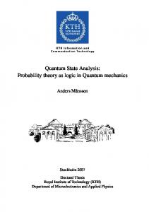
are partially ordered by refinement where a partition π = {B} refines a partition σ = {C}, written σ � π, if for any block B ∈ π, there is a block C ∈ σ such that B ⊆ C. The principal logical operation needed here is the partition join where the join π ∨ σ is the partition whose blocks are the non-empty intersections B ∩ C for B ∈ π and C ∈ σ. Each partition π can be represented as a binary relation dit (π) ⊆ U × U on U where the ordered pairs (u, u′ ) in dit (π) are the distinctions or dits of π in the sense that u and u′ are in distinct blocks of π. These dit sets dit (π) as binary relations might be called partition relations which are also called ”apartness relations” in computer science. An ordered pair (u, u′ ) is an indistinction or indit of π if u and u′ are in the same block of π. The set of indits, indit (π), as a binary relation is just the equivalence relation associated with the partition π, the complement of the dit set dit (π) in U × U . In the category-theoretic duality between sub-sets (which are the subject matter of Boole’s subset logic, the latter being usually mis-specified as the special case of ”propositional” logic) and quotient -sets or partitions ([6] or [10]), the elements of a subset and the distinctions of a partition are corresponding concepts.11 The partial ordering of subsets in the Boolean lattice ℘ (U ) is the Q inclusion of elements, and the refinement partial ordering of partitions in the partition lattice (U ) is just the inclusion of distinctions, i.e., σ � π iff dit (σ) ⊆ dit (π). The top of the Boolean lattice is the subset U of all possible elements and the top of the partition lattice is the discrete partition 1 = {{u}}u∈U of singletons which makes all possible distinctions: dit (1) = U × U − ∆ (where ∆ = {(u, u) : u ∈ U } is the diagonal). The bottom of the Boolean lattice is the empty set ∅ of no elements and the bottom of the lattice of partitions is the indiscrete partition (or blob) 0 = {U } which makes no distinctions. The two lattices can be illustrated in the case of U = {a, b, c}.
Figure 1: Subset and partition lattices In the correspondences between QM/sets and QM, a block S in a partition on U [i.e., a vector S ∈ ℘ (U )] corresponds to pure state in QM, and a partition π = {B} on U is the mixed state of orthogonal pure states B. In QM, a measurement makes distinctions, i.e., makes alternatives distinguishable, and that turns a pure state into a mixture of probabilistic outcomes. A measurement in QM/sets process of turning a pure state S ∈ ℘ (U ) into a mixed state � is the distinction-creating partition f −1 (r) ∩ S r∈f (U) on S. The distinction-creating process of measurement in QM/sets is � � the action on S of the inverse-image partition f −1 (r) r∈f (U) in the join {S, S c } ∨ f −1 (r) with the partition {S, S c }, so that action on S is: � S −→ f −1 (r) ∩ S r∈f (U) � Action on the pure state S of an f -measurement-join to give mixed state f −1 (r) ∩ S r∈f (U) on S. 11 Boole has been included along with Laplace in the name of classical finite probability theory since he developed it as the normalized counting measure on the elements of the subsets of his logic. Applying the same mathematical move to the dual logic of partitions results in developing the notion of logical entropy h (π) of a partition π as the normalized counting measure on the dit set dit (π), i.e., h (π) = |dit(π)| . ([5], [7]) |U ×U |
9
� The states f −1 (r) ∩ S r∈f (U) are all possible or ”potential” but the actual indefinite state S turns into one of the definite states with the probabilities given by the probability calculus: Pr(r|S) = 2 kf −1 (r)∩S kU |f −1 (r)∩S | . Since the reduction of the state S to the state f −1 (r)∩S is mathematically = |S| kSk2 U
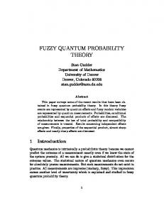
described by applying the projection operator f −1 (r) ∩ (), it is called a projective measurement. Hermann Weyl was at least one quantum theorist who touched on the relation between what was, in effect, QM/sets and QM. He called a partition a ”grating” or ”sieve,” and then considered both set partitions and vector space partitions (direct sum decompositions) as the respective types of gratings.[20, pp. 255-257] He started with a numerical attribute on a set, e.g., f : U → R, which defined � −1 the set partition or ”grating” [20, p. 255] with blocks having the same attribute-value, e.g., f (r) r∈f (U) . Then he moved to the QM case where the universe set, e.g., U = {u1 , ..., un }, or ”aggregate of n states has to be replaced by an n-dimensional Euclidean vector space” [20, p. 256]. The appropriate notion of a vector space partition or ”grating” is a ”splitting of the total vector → space into mutually orthogonal subspaces” so that ”each vector − x splits into r component vectors lying in the several subspaces” [20, p. 256], i.e., a direct sum decomposition of the space. After referring to a partition as a ”grating” or ”sieve,” Weyl notes that ”Measurement means application of a sieve �or grating” [20, p. 259], e.g., in QM/sets, the application (i.e.,�join) of the set-grating or partition f −1 (r) r∈f (U) to the pure state {S} to give the mixed state f −1 (r) ∩ S r∈f (U) . For some mental imagery of measurement, we might think of the grating as a series of regularpolygonal-shaped holes that might shape an indefinite blob of dough. In a measurement, the blob of dough falls through one of the polygonal holes with equal probability and then takes on that shape.
Figure 2: Measurement as randomly giving an indefinite blob of dough a definite polygonal shape.
4.2
Example of a nondegenerate measurement
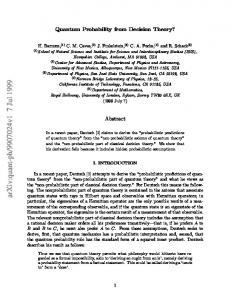
In the simple example illustrated below, we start at the one block or state of the indiscrete partition or blob which is the completely indistinct entity {a, b, c}. A measurement always uses some attribute that defines an inverse-image partition on U = {a, b, c}. In the case at hand, there are ”essentially” four possible attributes that could be used to ”measure” the indefinite entity {a, b, c} (since there are four partitions that refine the indiscrete partition in Figure 3). For an example of a nondegenerate measurement in QM/sets, consider any attribute f : U → R which has the discrete partition as its inverse image (i.e., is injective), such as the ordinal number of the letter in the alphabet: f (a) = 1, f (b) = 2, and f (c) = 3. This attribute has three (nonzero) eigenvectors: f ↾ {a} = 1 {a}, f ↾ {b} = 2 {b}, and f ↾ {c} = 3 {c} with the corresponding eigenvalues. The eigenvectors are {a}, {b}, and {c}, the blocks in the discrete partition of U . The nondegenerate measurement using the observable f acts on the pure state U = {a, b, c} to give the mixed state of the discrete partition 1: 10
� U → U ∩ f −1 (r) r=1,2,3 = 1. |f −1 (r)∩S | = Each such measurement would return an eigenvalue r with the probability of Pr (r|S) = |S| 1 for r ∈ f (U ) = {1, 2, 3}. 3 A projective measurement makes distinctions in the measured state that are sufficient to induce the ”quantum jump” or projection to the eigenvector associated with the observed eigenvalue. If the observed eigenvalue was 3, then the state {a, b, c} projects to f −1 (3)∩{a, b, c} = {c}∩{a, b, c} = {c} as pictured below.
Figure 3: Nondegenerate measurement and resulting ”quantum jump” It might be emphasized that this is a state reduction from the single indefinite state {a, b, c} to the single definite state {c}, not a subjective removal of ignorance as if the state had all along been {c}.
4.3
Example of a degenerate measurement
For an example of a degenerate measurement, we choose an attribute with a non-discrete inverseimage partition such as the partition π = {{a} , {b, c}}. Hence the attribute could just be the characteristic function χ{b,c} with the two eigenspaces ℘({a}) and ℘({b, c}) and the two eigenvalues � � 0 and 1 respectively. Since the eigenspace ℘ χ−1 {b,c} (1)
= ℘ ({b, c}) is not one dimensional, the
eigenvalue of 1 is a QM/sets-version of a degenerate eigenvalue. This attribute χ{b,c} has four (nonzero) eigenvectors: χ{b,c} ↾ {b, c} = 1 {b, c}, χ{b,c} ↾ {b} = 1 {b}, χ{b,c} ↾ {c} = 1 {c}, and χ{b,c} ↾ {a} = 0 {a}.
The ”measuring apparatus” makes distinctions by joining the attribute inverse-image partition n o −1 −1 χ−1 = χ (1) , χ (0) = {{b, c} , {a}} {b,c} {b,c} {b,c} with the pure state representing the indefinite entity U = {a, b, c}. The action on the pure state is: −1 U → {U } ∨ χ−1 {b,c} = χ{b,c} = {{b, c} , {a}}.
The measurement of that attribute returns one of the eigenvalues with the probabilities: Pr(0|U ) =
|{a}∩{a,b,c}| |{a,b,c}|
=
1 3
and Pr (1|U ) =
|{b,c}∩{a,b,c}| |{a,b,c}|
= 23 .
Suppose it returns the eigenvalue 1. Then the indefinite entity {a, b, c} reduces to the projected eigenstate χ−1 {b,c} (1) ∩ {a, b, c} = {b, c} for that eigenvalue [3, p. 221].
11
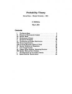
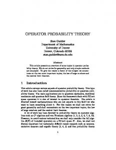
� � Since this is a degenerate result (i.e., the eigenspace ℘ χ−1 = ℘ ({b, c}) doesn’t have {b,c} (1) dimension one), another measurement is needed to make more distinctions. Measurements by attributes, such as χ{a,b} or χ{a,c} , that give either of the other two partitions, {{a, b} , {c}} or {{b} , {a, c}} as inverse images, would suffice to distinguish {b, c} into {b} or {c}. Then either attribute together with the attribute χ{b,c} would form a Complete Set of Compatible Attributes or CSCA (i.e., the QM/sets-version of a Complete Set of Commuting Operators or CSCO [4]), where complete means that the join of the attributes’ inverse-image partitions gives the discrete partition and where compatible means that all the attributes can be taken as defined on the same set of (simultaneous) basis eigenvectors, e.g., the U -basis. Taking, for example, the other attribute as χ{a,b} , the join of the two attributes’ partitions is discrete: −1 χ−1 {b,c} ∨ χ{a,b} = {{a} , {b, c}} ∨ {{a, b} , {c}} = {{a} , {b} , {c}} = 1.
Hence all the eigenstate singletons can be characterized by the ordered pairs of the eigenvalues of these two attributes: {a} = |0, 1i, {b} = |1, 1i, and {c} = |1, 0i (using Dirac’s ket-notation to give the ordered pairs and listing the eigenvalues of χ{b,c} first on the left). The second projective measurement of the indefinite entity {b, c} using the attribute χ{a,b} with the inverse-image partition χ−1 {a,b} = {{a, b} , {c}} would have the pure-to-mixed state action: � {b, c} → {b, c} ∩ χ{a,b} (1), {b, c} ∩ χ{a,b} (0) = {{b} , {c}}.
The distinction-making measurement would cause the indefinite entity {b, c} to turn into one of the definite entities of {b} or {c} with the probabilities: Pr (1| {b, c}) =
|{a,b}∩{b,c}| |{b,c}|
=
1 2
and Pr (0| {b, c}) =
|{c}∩{b,c}| |{b,c}|
= 21 .
If the measured eigenvalue is 0, then the state {b, c} projects to χ−1 {a,b} (0) ∩ {b, c} = {c} as pictured below.
Figure 4: Degenerate measurement The two projective measurements of {a, b, c} using the complete set of compatible (e.g., both defined on U ) attributes χ{b,c} and χ{a,b} produced the respective eigenvalues 1 and 0 so the resulting eigenstate was characterized by the eigenket |1, 0i = {c}. Again, this is all analogous to standard Dirac-von-Neumann quantum mechanics.
4.4
Measurement using density matrices
The previous treatment of the role of partitions in measurement can be restated using density matrices [17, p. 98] over the reals. Given a partition π = {B} on U = {u1 , ..., un }, the blocks B ∈ π can be thought of as (nonoverlapping or ”orthogonal”) ”pure states” where the ”state” B occurs with 12
the probability pB = |B| |U| . Then we can mimic the usual procedure for forming the density matrix ρ (π) for the ”orthogonal pure states” B with the probabilities pB . The ”pure state” B normalized in the reals to length 1 is represented by the column vector |Bi1 = √1 [χB (u1 ) , ..., χB (un )]t (where []t |B|
indicates the transpose). Then the density matrix ρ (B) for the pure state B ⊆ U is then (calculating in the reals): χB (u1 ) χB (u2 ) t 1 ρ (B) = |Bi1 (|Bi1 ) = |B| [χB (u1 ) , ..., χB (un )] .. .
χB (u1 ) χB (u2 ) χB (u1 ) 1 = |B| .. .
χB (un ) χB (u1 ) χB (u2 ) χB (u2 ) .. .
χB (un ) χB (u1 ) χB (un ) χB (u2 )
··· ··· .. .
···
χB (u1 ) χB (un ) χB (u2 ) χB (un ) . .. . χB (un )
For instance if U = {u1 , u2 , u3 }, then for the blocks in the partition 1 1 0 0 0 2 2 ρ ({u1 , u2 }) = 12 21 0 and ρ ({u3 }) = 0 0 0 0 0 0 0
π = {{u1 , u2 } , {u3 }}: 0 0. 1
Then the ”mixed state” density matrix ρ (π) of the partition π is the weighted sum: P ρ (π) = B∈π pB ρ (B). In the example, this is:
ρ (π) =
1
2 2 1 2 3
0
1 2 1 2
0
0 0 + 0
0 0 1 0 0 3 0 0
1 0 3 0 = 13 0 1
1 3 1 3
0
0 0 . 1 3
While this construction mimics the usual construction of the density matrix for orthogonal pure states, the remarkable thing is that the entries have a direct interpretation in terms of the dits and indits of the partition π: � 1 |U| if (uj , uk ) ∈ indit (π) . ρjk (π) = 0 if (uj , uk ) ∈ / indit (π) All the entries are real ”amplitudes” whose squares are the two-draw probabilities of drawing a pair of elements from U (with replacement) that is anq indistinction of π. As in the quantum case, the 1 1 1 non-zero entries of the density matrix ρjk (π) = |U| |U| = |U| are the ”coherences” [3, p. 302] which indicate that uj and uk ”cohere” together in a block or ”pure state” of the partition, i.e., (uj , uk ) ∈ indit (π). Since the ordered pairs (uj , uj ) in the diagonal ∆ ⊆ U × U are always indits of 1 . any partition, the diagonal entries in ρ (π) are always |U| Combinatorial theory gives another way to define the density matrix of a partition. A binary relation R ⊆ U × U on U = {u1 , ..., un } can be represented by an n × n incidence matrix I(R) where � 1 if (ui , uj ) ∈ R I (R)ij = 0 if (ui , uj ) ∈ / R. Taking R as the equivalence relation indit (π) associated with a partition π, the density matrix ρ (π) defined above is just the incidence matrix I (indit (π)) normalized to be of trace 1 (sum of diagonal entries is 1): 13
ρ (π) =
1 |U| I
(indit (π)). t
If the subsets T ∈ ℘ (U ) are represented by the n-ary column vectors [χT (u1 ) , ..., χT (un )] , then the action of the projection operator B ∩ () : ℘ (U ) → ℘ (U ) is represented by the n × n diagonal matrix PB where the diagonal entries are: � 1 if ui ∈ B (PB )ii = = χB (ui ) 0 if ui ∈ /B which is idempotent, PB2 = PB , and symmetric, PBt = PB . For any state S ∈ ℘ (U ), the trace (sum of diagonal entries) of PB ρ (S) is: tr [PB ρ (S)] = so given f : U → R,
1 |S|
Pn
Pr (r|S) =
i=1
χS (ui ) χB (ui ) =
|f −1 (r)∩S | |S|
|B∩S| |S|
= Pr (B|S)
� � = tr Pf −1 (r) ρ (S) .
We saw previously how the action of a measurement in QM/sets could be described using the partition join S operation. The join π ∨ σ of the partitions π = {B} and σ = {C} could be seen as the result C∈σ {C ∩ B 6= ∅ : B ∈ π} of the projection operators C ∩ () acting on the B ∈ π for all t C ∈ σ. Substituting the normalized |Bi1 for B with the density matrix ρ (B) = |Bi1 (|Bi1 ) and the matrix projection operators PC for C ∩ (), the application of PC to |Bi1 yields the density matrix: (PC |Bi1 ) (PC |Bi1 )t = PC |Bi1 (|Bi1 )t PCt = PC ρ (B) PC . P Summing with the probability weights gives: PB∈π pB PC ρ (B) PC = PC ρ (π) PC and then summing over the different projection operators gives: C∈σ PC ρ (π) PC . A little calculation then shows that this is exactly the density matrix of the partition join: P C∈σ PC ρ (π) PC = ρ (π ∨ σ). Density matrix version of the partition join We are modeling, using density matrices, the QM/sets projective measurement of an attribute f : U → R starting with a pure state S. Then measurement converts the pure state |Si to one of � −1 (r)∩S| the states f −1 (r) ∩ S with the probability |f |S| . In the previous example of a (degenerate) measurement with U = {a, b, c} and f = χ{b,c} , then the measurement, in terms nof partitions, had o � −1 −1 the effect of making distinctions on the partition {U } by the partition f = χ{b,c} using the join operation: n o {U } → {U } ∨ χ−1 {b,c} = {{b, c} , {a}}. −1 The mixed state {{b, c} , {a}} has the projected outcomes χ−1 {b,c} (1) ∩ U = {b, c} and χ{b,c} (0) ∩ U = {a} which occur with the probabilities Pr (1|U ) = χ−1 {b,c} (1) ∩ U / |U | = 2/3 and Pr (0|U ) = −1 χ{b,c} (0) ∩ U / |U | = 1/3. We now have the density matrix version of the partition join operation, so in the general case c of starting with the pure state S, we might take starting � −1 the � −1 partition on U as π = {S, S } and then take the measurement join with σ = f = f (r) r∈f (U) which yields the density matrix (using linearity):
14
� � P ρ {S, S c } ∨ f −1 = r∈f (U) Pf −1 (r) ρ ({S, S c }) Pf −1 (r) P P = pS r∈f (U) Pf −1 (r) ρ (S) Pf −1 (r) + pS c r∈f (U) Pf −1 (r) ρ (S c ) Pf −1 (r) . t
Thus starting with the pure state density matrix ρ (S) = |Si1 (|Si1 ) , the action of the measurement given by the partition join (ignoring the action on the complement S c ) is to create the mixed state ρˆ (S): ρ (S) −→ ρˆ (S) =
P
r∈f (U)
Pf −1 (r) ρ (S) Pf −1 (r)
Action of measurement of attribute f on the pure state density matrix ρ (S). � In that mixed state, the projected state f −1 (r) ∩ S occurs with the probability tr[Pf −1 (r) ρ (S)] = |f −1 (r)∩S| |S|
= Pr (r|S). In full QM, the projective Pm measurement using a Hermitian observable operator L with the spectral decomposition L = i=1 λi Pi of a normalized pure state |ψi results in the state Pi |ψi with the probability pi = tr [Pi ρ (ψ)] = Pr (λi |ψ) where ρ (ψ) = |ψi hψ|. The projected resultant state Pi ρ(ψ)Pi i |ψihψ|Pi Pi |ψi has the density matrix Ptr[P = tr[P so the mixed state describing the probabilistic i ρ(ψ)] i ρ(ψ)] results of the measurement is [17, p. 101]: P P P Pi ρ(ψ)Pi Pi ρ(ψ)Pi = i tr [Pi ρ (ψ)] tr[P = i Pi ρ (ψ) Pi . ρˆ (ψ) = i pi tr[P i ρ(ψ)] i ρ(ψ)]
Thus we see how the density matrix treatment of measurement in QM/sets is just a sets-version of the density matrix treatment of projective measurement in standard Dirac-von-Neumann QM. And we have the additional philosophically-relevant information that the measurement is described by the distinction-creating partition join operation in QM/sets–which confirms the observation in QM that the essence of measurement is distinguishing the alternative possible states. For instance, Richard Feynman always emphasized the importance of distinctions as characterizing what amounts to a ”measurement.” If you could, in principle, distinguish the alternative final states (even though you do not bother to do so), the total, final probability is obtained by calculating the probability for each state (not the amplitude) and then adding them together. If you cannot distinguish the final states even in principle, then the probability amplitudes must be summed before taking the absolute square to find the actual probability.[12, p. 3.9]
4.5
Quantum dynamics and the two-slit experiment in QM/sets
To illustrate a two-slit experiment in quantum mechanics over sets, we need to introduce some ”dynamics.” In quantum mechanics, the no-distinctions requirement is that the linear transformation has to preserve the degree of indistinctness hψ|ϕi, i.e., that it preserved the inner product. Where two normalized states are fully distinct if hψ|ϕi = 0 and fully indistinct if hψ|ϕi = 1, it is also sufficient to just require that full distinctness and indistinctness be preserved since that would imply orthonormal bases are preserved and that is equivalent to being unitary. In QM/sets, we have no inner product but the idea of a linear transformation A : Zn2 → Zn2 preserving distinctness would simply The condition analogous to preserving inner product is
mean being non-singular. � hS|U T i = A (S) |A(U) A (T ) where A (U ) = U ′ is defined by A ({u}) = {u′ }. For non-singular A, the image A (U ) of the U -basis is a basis, i.e., the U ′ -basis, and the ”bracket-preserving” condition holds since |S ∩ T | = |A (S) ∩ A (T )| for A (S) , A (T ) ⊆ A (U ) = U ′ . Hence the QM/sets analogue of the unitary dynamics of full QM is ”non-singular dynamics,” i.e., the change-of-state matrix is non-singular.12 12 In Schumacher and Westmoreland’s modal quantum theory [18], they also take the dynamics to be any nonsingular linear transformation.
15
Consider the dynamics given in terms of the U -basis where: {a} → {a, b}; {b} → {a, b, c}; and {c} → {b, c} in one time period. This is represented by the non-singular one-period change of state matrix: 1 1 0 A = 1 1 1. 0 1 1 The seven nonzero vectors in the vector space are divided by this ”dynamics” into a 4 -orbit: {a} → {a, b} → {c} → {b, c} → {a}, a 2-orbit: {b} → {a, b, c} → {b}, and a 1-orbit: {a, c} → {a, c}. If we take the U -basis vectors as ”vertical position” eigenstates, we can device a QM/sets version of the ”two-slit experiment” which models ”all of the mystery of quantum mechanics” [11, p. 130]. Taking a, b, and c as three vertical positions, we have a vertical diaphragm with slits at a and c. Then there is a screen or wall to the right of the slits so that a ”particle” will travel from the diaphragm to the wall in one time period according to the A-dynamics.
Figure 5: Two-slit setup We start with or ”prepare” the state of a particle being at the slits in the indefinite position state {a, c}. Then there are two cases. First case of distinctions at slits: The first case is where we measure the U -state at the slits and then let the resultant position eigenstate evolve by the A-dynamics to hit the wall at the right where the position is measured again. The probability that the particle is at slit 1 or at slit 2 is: Pr ({a} measured at slits | {a, c} at slits) = Pr ({c} measured at slits | {a, c} at slits) =
h{a}|U {a,c}i2 k{a,c}k2U h{c}|U {a,c}i2 k{a,c}k2U
= =
|{a}∩{a,c}| |{a,c}| |{c}∩{a,c}| |{a,c}|
= 21 ; = 12 .
If the particle was at slit 1, i.e., was in eigenstate {a}, then it evolves in one time period by the A-dynamics to {a, b} where the position measurements yield the probabilities of being at a or at b as:
Pr ({a} measured at wall | {a, b} at wall) = Pr ({b} measured at wall | {a, b} at wall) =
h{a} |U {a, b}i2 2 k{a, b}kU
|{a} ∩ {a, b}| 1 = |{a, b}| 2
=
1 |{b} ∩ {a, b}| = . |{a, b}| 2
2
h{b} |U {a, b}i 2 k{a, b}kU
=
If on the other hand the particle was found in the first measurement to be at slit 2, i.e., was in eigenstate {c}, then it evolved in one time period by the A-dynamics to {b, c} where the position measurements yield the probabilities of being at b or at c as: 16
Pr ({b} measured at wall | {b, c} at wall) =
Pr ({c} measured at wall | {b, c} at wall) =
|{b}∩{b,c}| |{b,c}| |{c}∩{b,c}| |{b,c}|
= =
1 2 1 2.
Hence we can use the laws of probability theory to compute the probabilities of the particle being measured at the three positions on the wall at the right if it starts at the slits in the superposition state {a, c} and the measurements were made at the slits: Pr({a} measured at wall | {a, c} at slits) = 21 21 = 14 ; Pr({b} measured at wall | {a, c} at slits) = 12 21 + 21 21 = 12 ; Pr({c} measured at wall | {a, c} at slits) = 12 21 = 41 .
Figure 6: Final probability distribution with measurements at slits Second case of no distinctions at slits: The second case is when no measurements are made at the slits and then the superposition state {a, c} evolves by the A-dynamics to {a, b}+{b, c} = {a, c} where the superposition at {b} cancels out. Then the final probabilities will just be probabilities of finding {a}, {b}, or {c} when the measurement is made only at the wall on the right is: Pr({a} measured at wall | {a, c} at slits) = Pr ({a} | {a, c}) = Pr({b} measured at wall | {a, c} at slits) = Pr ({b} | {a, c}) =
Pr({c} measured at wall | {a, c} at slits) = Pr ({c} | {a, c}) =
|{a}∩{a,c}| = 12 ; |{a,c}| |{b}∩{a,c}| = 0; |{a,c}| |{c}∩{a,c}| = 12 . |{a,c}|
Figure 7: Final probability distribution with no measurement at slits Since no ”collapse” took place at the slits due to no distinctions being made there, the indistinct element {a, c} evolved (rather than one or the other of the distinct elements {a} or {c}). The action of A is the same on {a} and {c} as when they evolve separately since A is a linear operator but 17
the two results are now added together as part of the evolution. This allows the ”interference” of the two results and thus the cancellation of the {b} term in {a, b} + {b, c} = {a, c}. The addition is, of course, mod 2 (where −1 = +1) so, in ”wave language,” the two ”wave crests” that add at the location {b} cancel out. When this indistinct element {a, c} ”hits the wall” on the right, there is an equal probability of that distinction yielding either of those eigenstates. Figure 7 shows the simplest example of the ”light and dark bands” characteristic of superposition and interference illustrating ”all of the mystery of quantum mechanics”. This pedagogical model gives the simple logical essence of the two-slit experiment without the complex-valued wave functions that distract from the essential point–which is the difference between the separate mixed state evolutions resulting from measurement at the slits, and the combined evolution of the superposition {a, c} that allows interference (without ”waves”).
5
Further steps
Showing that ordinary Laplace-Boole finite probability theory is the quantum probability calculus for the pedagogical or ”toy” model, quantum mechanics over sets (QM/sets), is only an initial part of a research programme. For instance, we have not considered: • the whole ”non-commutative” side of viewing the Laplace-Boole theory in the context of vector spaces over Z2 where the compatibility of numerical attributes f : U → R and g : U ′ → R defined on different equicardinal basis sets {u} ⊆ U and {u′ } ⊆ U ′ can be analyzed in terms of the commutativity of all the associated projection operators f −1 (r) ∩ () and g −1 (s) ∩ () on Zn2 [8]; or • the treatment of entanglement in QM/sets which reduces to some old-fashioned correlation in the equiprobability distribution on a state that is a subset of a Cartesian product but which still allows a Bell-type result to be established [9]. Our purpose here is limited to showing how the perfectly classical Laplace-Boole finite probability theory is the quantum probability calculus of the pedagogical model of quantum mechanics over sets. The point is not to clarify finite probability theory but to elucidate quantum mechanics itself by seeing some of its quantum features formulated in a classical setting.
References [1] Abramsky, Samson and Coecke, Bob 2004. A categorical semantics of quantum protocols. in: Proceedings of the 19th IEEE Symposium on Logic in Computer Science (LiCS’04), IEEE Computer Science Press, 415–425 . [2] Boole, George 1854. An Investigation of the Laws of Thought on which are founded the Mathematical Theories of Logic and Probabilities. Cambridge: Macmillan and Co. [3] Cohen-Tannoudji, Claude, Bernard Diu and Franck Lalo¨e 2005. Quantum Mechanics Vol. 1. New York: John Wiley & Sons. [4] Dirac, Paul A. M. 1958. The Principles of Quantum Mechanics (4th ed.). Oxford: Clarendon. [5] Ellerman, David 2009. Counting Distinctions: On the Conceptual Foundations of Shannon’s Information Theory. Synthese. 168 (1 May): 119-149. [6] Ellerman, David 2010. The Logic of Partitions: Introduction to the Dual of the Logic of Subsets. Review of Symbolic Logic. 3 (2 June): 287-350.
18
[7] Ellerman, David 2013. An Introduction to Logical Entropy and its Relation to Shannon Entropy. International Journal of Semantic Computing, 7(2): 121-145. [8] Ellerman, David 2013. The Objective Indefiniteness Interpretation of Quantum Mechanics, [quant-ph] arXiv:1210.7659. [9] Ellerman, David 2013. Quantum mechanics over sets. arXiv:1310.8221 [quant-ph]. [10] Ellerman, David 2014. An Introduction of Partition Logic. Logic Journal of the IGPL. 22, no. 1: 94–125. [11] Feynman, Richard P. 1967. The Character of Physical Law. Cambridge: MIT Press. [12] Feynman, Richard P., Robert B. Leighton, and Matthew Sands 1965. The Feynman Lectures on Physics: Quantum Mechanics (Vol. III). Reading MA: Addison-Wesley. [13] Hanson, Andrew J., Gerardo Ortiz, Amr Sabry, and Yu-Tsung Tai 2013. Discrete Quantum Theories. arXiv:1305.3292v1. [14] Jammer, Max 1966. The Conceptual Development of Quantum Mechanics. New York: McGrawHill. [15] Laplace, Pierre-Simon. 1995 (1825). Philosophical Essay on Probabilities. Translated by A. I. Dale. New York: Springer-Verlag. [16] McEliece, Robert J. 1977. The Theory of Information and Coding: A Mathematical Framework for Communication (Encyclopedia of Mathematics and its Applications, Vol. 3). Reading MA: Addison-Wesley. [17] Nielsen, M., and I. Chuang. 2000. Quantum Computation and Quantum Information. Cambridge: Cambridge University Press. [18] Schumacher, Benjamin and Michael Westmoreland 2012. Modal Quantum Theory. Foundations of Physics, 42, 918-925. [19] Takeuchi, T., L.N. Chang, Z. Lewis, and D. Minic. 2012. Some Mutant Forms of Quantum Mechanics. [quant-Ph] arXiv:1208.5544v1. [20] Weyl, Hermann 1949. Philosophy of Mathematics and Natural Science. Princeton NJ: Princeton University Press.
19