2.7 Symbolic Computation in PDE Solving Environments : : : : : : : : : 39 ..... issues that arise when developing software for such applications. Finally, we introduce.
PROBLEM SOLVING ENVIRONMENTS FOR PARTIAL DIFFERENTIAL EQUATION BASED APPLICATIONS A Thesis Submitted to the Faculty of Purdue University by Sanjiva Weerawarana In Partial Ful llment of the Requirements for the Degree of Doctor of Philosophy August 1994
ii
This thesis is dedicated to my parents, Kamal and Ruby Fernando, without whose lifelong advice, guidance, encouragement, trust, patience and unbounded love my academic career could never have reached this point.
iii
ACKNOWLEDGMENTS It is a pleasure to take this opportunity to attempt to recognize all the people who helped me get through my (sometimes di�cult) doctoral student years! Since I can only name so many people, I will start by saying \Thank You!" to all my wonderful friends, teachers and of course relatives. I am very sorry that I cannot acknowledge you individually, but the appreciation I have for what you all did for me is nonetheless limitless! Of course, my wonderful advisor Prof. Elias N. Houstis is the catalyst to almost every good thing that happened to me in the last several years. A short paragraph cannot possibly acknowledge all that he has done for me; Elias Houstis was much more than an academic advisor to me in these years. To Elias, I owe eternal gratitude, in nite respect and lifelong friendship for (extremely patiently) moulding a researcher out of me! Prof. John R. Rice also provided much inspiration during my time in the CAPO, SoftLab and PDELab groups. His careful scrutinization of my thesis helped it immensely and the many discussions with him taught me to not always worry about details! The other two members of my examining committee, Prof. Vincent F. Russo and Prof. Ahmed K. Elmagarmid, also helped me in many ways with the suggestions and comments about my work. Being a part of the CAPO, SoftLab and PDELab groups has been an absolute pleasure for me. Ann Christine, Shahani, Amy, Sang{Bae, Cheryl, Stephen, Po Ting, Kostas, Nick (Houstis), Tzvetan, Anupam, Ben, Margaret and Mei{Ling and past members, Panos, Ko Yang, Nick (Chrisochoides), Reggie, Yu{Ling, Manolis, Pelayia, Jim, Scott and Hyeran have all contributed to my work with all the discussions we've
iv had about how to solve PDEs. Ann Christine needs special mention; thanks so much for all your invaluable help, advice and encouragement, Ann Christine! If I didn't acknowledge the group of Sri Lankan friends with whom I spent many an evening, then I'd be doing a great injustice. Our late night sessions coming up with solutions to all the problems of the world (after a few rounds, of course) and the volatile walleyball sessions were probably the most therapeutic things I did during these years! To Yohan, Nishantha, Kirthi, my little sister Santhani, Niranjan, Athula, Rajee and of course my wife Shahani, \Thank you!", I will never forget these great years! Now to the people closest to me{ of course, none of this would ever have been possible had my family not allowed me to come to the US in 1985. I do not have the right words to acknowledge my father Kamal, my mother Ruby, my elder sister Kumari, my younger sister Santhani and my brother{in{law Varuna, so I will simply say \Thank you!" Your support never waivered (even when I was terribly waivering : : : ) and you never stopped telling me to keep going { I know I couldn't have done it without your help! Finally, and obviously the most, I come to my beloved wife, Shahani Markus. Even though we've been married only for a bit over two years, we've known each other since just two hours after I drove over to Purdue in 1989. Shahani has been a big part of my life and my Ph.D. for much longer than two years and has had to tolerate all my bickering about them. For all the patience, kindness, advice and love you have given me, I thank you. For putting up with all the stu� that I've been throwing at you (not literally, of course!) for the last several years, I thank you. For staying up with me the night before my defense and teaching me those wonderful German things so that I could pass the language exam the next morning, I thank you (big time)! As I cannot possibly explain all the little things that you did for me, I will just say \I simply couldn't have done it without you, period!"
v Really nally, I wish to acknowledge all the generous funding agencies that made my work logistically possible: Purdue University, Purdue University Foundation, Purdue University Research Foundation, Intel Foundation, National Science Foundation, Air Force O�ce of Scienti c Research, Advanced Research Projects Agency, and my parents' bank account.
vi
TABLE OF CONTENTS Page LIST OF TABLES : : : : : : : : : : : : : : : : : : : : : : : : : : : : : : : : :
x
LIST OF FIGURES : : : : : : : : : : : : : : : : : : : : : : : : : : : : : : : :
xi
ABSTRACT : : : : : : : : : : : : : : : : : : : : : : : : : : : : : : : : : : : : xvi 1. INTRODUCTION : : : : : : : : : : : : : : : : : : : : : : : : : : : : : : : 1.1 Modeling with Partial Di�erential Equations : : 1.2 Evolution of PDE Solving Software : : : : : : : 1.3 Problem Solving Environments : : : : : : : : : 1.3.1 Properties of PSEs : : : : : : : : : : : : 1.3.2 PSEs vs. PSE Frameworks : : : : : : : : 1.4 PDE Based Applications and Application PSEs 1.4.1 The PDELab Prototype : : : : : : : : : 1.5 Overview of the Thesis : : : : : : : : : : : : : :
: : : : : : : :
: : : : : : : :
: : : : : : : :
1 3 8 8 9 10 11 12
2. THE ARCHITECTURE OF A SOFTWARE FRAMEWORK FOR BUILDING PROBLEM SOLVING ENVIRONMENTS FOR PDE BASED APPLICATIONS : : : : : : : : : : : : : : : : : : : : : : : : : : : : : : : : : : : :
13
2.1 Introduction : : : : : : : : : : : : : : : : : : : : : : 2.2 Related Work : : : : : : : : : : : : : : : : : : : : : 2.2.1 PDE Solving Software Environments : : : : 2.2.2 Application Development Frameworks : : : 2.2.3 Software Bus Environments : : : : : : : : : 2.3 Design Objectives of PDELab : : : : : : : : : : : : 2.4 Software Architecture : : : : : : : : : : : : : : : : : 2.4.1 Algorithms and Systems Infrastructure : : : 2.4.2 Software Infrastructure : : : : : : : : : : : : 2.4.3 PSE Development Framework : : : : : : : : 2.4.4 Application Problem Solving Environments :
: : : : : : : :
: : : : : : : : : : :
: : : : : : : :
: : : : : : : : : : :
: : : : : : : :
: : : : : : : : : : :
: : : : : : : :
: : : : : : : : : : :
: : : : : : : :
: : : : : : : : : : :
: : : : : : : :
: : : : : : : : : : :
: : : : : : : :
: : : : : : : : : : :
: : : : : : : :
: : : : : : : : : : :
: : : : : : : :
1
: : : : : : : : : : :
: : : : : : : : : : :
13 16 16 18 20 21 21 23 25 26 27
vii Page 2.5 Communication: The PDELab Software Bus : : : : : : 2.5.1 Requirements: Clients, Protocols and Services : 2.5.2 Bus Architecture : : : : : : : : : : : : : : : : : 2.5.3 Con guring a New PSE : : : : : : : : : : : : : 2.5.4 Comparison with Software Bus Reference Model 2.5.5 Why Yet Another Communication Library? : : 2.6 PSE Development Framework : : : : : : : : : : : : : : 2.6.1 PDE Object Editors : : : : : : : : : : : : : : : 2.6.2 Worksheet Editor : : : : : : : : : : : : : : : : : 2.6.3 PDESpec Language : : : : : : : : : : : : : : : : 2.6.4 PYTHIA Environment : : : : : : : : : : : : : : 2.6.5 Component Composition : : : : : : : : : : : : : 2.7 Symbolic Computation in PDE Solving Environments : 2.7.1 Symbolic Computation in PDELab : : : : : : : 2.7.2 Implementation : : : : : : : : : : : : : : : : : : 2.8 Example: Integrating a New Solver : : : : : : : : : : : 2.9 Example: The Bioseparation Workbench : : : : : : : : 2.10 Conclusion : : : : : : : : : : : : : : : : : : : : : : : : :
: : : : : : : : : : : : : : : : : :
: : : : : : : : : : : : : : : : : :
: : : : : : : : : : : : : : : : : :
: : : : : : : : : : : : : : : : : :
: : : : : : : : : : : : : : : : : :
: : : : : : : : : : : : : : : : : :
: : : : : : : : : : : : : : : : : :
: : : : : : : : : : : : : : : : : :
27 28 29 31 32 33 34 35 36 38 38 39 39 39 41 42 45 47
3. HIGH LEVEL LANGUAGE FOR PARTIAL DIFFERENTIAL EQUATION BASED MATHEMATICAL MODELS AND THEIR SOLUTIONS : : : : 48 3.1 Introduction : : : : : : : : : : : : : : : : : : : : : : : 3.2 Related Work : : : : : : : : : : : : : : : : : : : : : : 3.2.1 Program Translation{Type Languages : : : : 3.2.2 Code Generation Based Languages : : : : : : 3.3 Approach and Rationale : : : : : : : : : : : : : : : : 3.4 Speci cation of PDE Models : : : : : : : : : : : : : : 3.4.1 Domains : : : : : : : : : : : : : : : : : : : : : 3.4.2 PDE Operator Equations : : : : : : : : : : : 3.4.3 Boundary Conditions : : : : : : : : : : : : : : 3.4.4 Initial Conditions : : : : : : : : : : : : : : : : 3.5 Discrete Geometries and Geometry Decompositions : 3.6 Speci cation of PDE Solution Schemes : : : : : : : : 3.7 Representing PDE Solutions : : : : : : : : : : : : : : 3.8 Syntax and Semantics of PDESpec : : : : : : : : : : 3.8.1 Basic Syntax : : : : : : : : : : : : : : : : : : 3.8.2 Overview of Syntax and Semantics : : : : : : 3.8.3 Example: The Algorithm Object : : : : : : : 3.9 Implementation : : : : : : : : : : : : : : : : : : : : : 3.9.1 Representing the PDE Problem Components : 3.9.2 Representing Discrete Geometries : : : : : : :
: : : : : : : : : : : : : : : : : : : :
: : : : : : : : : : : : : : : : : : : :
: : : : : : : : : : : : : : : : : : : :
: : : : : : : : : : : : : : : : : : : :
: : : : : : : : : : : : : : : : : : : :
: : : : : : : : : : : : : : : : : : : :
: : : : : : : : : : : : : : : : : : : :
: : : : : : : : : : : : : : : : : : : :
: : : : : : : : : : : : : : : : : : : :
48 51 51 52 53 55 56 57 58 58 58 60 62 63 63 63 65 68 68 69
viii Page 3.9.3 Translating Algorithms : : : : : : : : : : : : : : : 3.9.4 Execution : : : : : : : : : : : : : : : : : : : : : : 3.9.5 Representing Computed Solutions : : : : : : : : : 3.10 Symbolic Manipulation in PDESpec : : : : : : : : : : : : 3.10.1 Symbolic Transformations : : : : : : : : : : : : : 3.10.2 Representation Translation and Code Generation 3.11 Examples : : : : : : : : : : : : : : : : : : : : : : : : : : 3.11.1 Steady{State Heat Flow in a Reactor : : : : : : : 3.11.2 Modeling the Drying and Shrinkage of Salami : : 3.12 Conclusion : : : : : : : : : : : : : : : : : : : : : : : : : :
: : : : : : : : : :
: : : : : : : : : :
69 70 70 70 71 72 73 73 77 82
4. COMPUTATIONAL INTELLIGENCE FOR PROBLEM SOLVING ENVIRONMENTS : : : : : : : : : : : : : : : : : : : : : : : : : : : : : : : : : :
84
4.1 Introduction : : : : : : : : : : : : : : : : : : : : : : : : : : 4.2 Related Work : : : : : : : : : : : : : : : : : : : : : : : : : 4.3 An Overview of PYTHIA : : : : : : : : : : : : : : : : : : 4.3.1 The PDE Solver Selection Problem : : : : : : : : : 4.3.2 PDE Problem Characteristics : : : : : : : : : : : : 4.3.3 Population of Elliptic PDEs : : : : : : : : : : : : : 4.3.4 Performance Knowledge for Elliptic PDE Solvers : 4.4 The PYTHIA Knowledge Bases : : : : : : : : : : : : : : : 4.4.1 Facts : : : : : : : : : : : : : : : : : : : : : : : : : : 4.4.2 Rules : : : : : : : : : : : : : : : : : : : : : : : : : : 4.5 The Inference Algorithm : : : : : : : : : : : : : : : : : : : 4.6 Dealing with Uncertainty : : : : : : : : : : : : : : : : : : : 4.6.1 Evidence Nodes F1, : : : , Fn: Problem Features : : : 4.6.2 Node C : Finding Closest Classes : : : : : : : : : : 4.6.3 Node P : Finding Closest Problems : : : : : : : : : 4.6.4 Evidence Node I : Performance Criteria Weights : : 4.6.5 Evidence Node R: Method Rank Weight : : : : : : 4.6.6 Evidence Node E : Error Level Weights : : : : : : : 4.6.7 Node M : Determining the Best Method : : : : : : 4.6.8 Node O: Generating Output : : : : : : : : : : : : : 4.7 Using Neural Networks : : : : : : : : : : : : : : : : : : : : 4.8 Architecture and Implementation : : : : : : : : : : : : : : 4.8.1 CLIPS: C Language Integrated Production System 4.8.2 The Knowledge Engineering Environment : : : : : 4.8.3 The Consultation Environment : : : : : : : : : : : 4.9 Performance Evaluation of PYTHIA : : : : : : : : : : : : 4.9.1 Class Selection Using Neural Networks : : : : : : : 4.9.2 Method Selection and Parameter Prediction : : : :
: : : : : : : : : :
: : : : : : : : : : : : : : : : : : : : : : : : : : : :
: : : : : : : : : :
: : : : : : : : : : : : : : : : : : : : : : : : : : : :
: : : : : : : : : :
: : : : : : : : : : : : : : : : : : : : : : : : : : : :
: : : : : : : : : :
: : : : : : : : : : : : : : : : : : : : : : : : : : : :
: : : : : : : : : :
: : : : : : : : : : : : : : : : : : : : : : : : : : : :
: : : : : : : : : : : : : : : : : : : : : : : : : : : :
85 86 88 88 90 91 93 94 94 97 101 106 106 107 107 107 108 108 108 109 109 112 112 112 115 116 116 122
ix Page 4.9.3 The Overhead of PYTHIA : : : : : : : : : : : : : : : : : : : : 123 4.10 Conclusion : : : : : : : : : : : : : : : : : : : : : : : : : : : : : : : : : 124 5. SOFTLAB: TOWARDS A VIRTUAL LABORATORY FOR SCIENCE : : 126 5.1 Introduction : : : : : : : : : : : : : : : : : : : : : : : : : : : : : : : 5.2 Related Work : : : : : : : : : : : : : : : : : : : : : : : : : : : : : : 5.3 The SoftLab Vision : : : : : : : : : : : : : : : : : : : : : : : : : : : 5.3.1 Functionality : : : : : : : : : : : : : : : : : : : : : : : : : : 5.3.2 Usage Scenarios : : : : : : : : : : : : : : : : : : : : : : : : : 5.4 Implementation of SoftLab : : : : : : : : : : : : : : : : : : : : : : : 5.4.1 Gathering Experimental Data and Controlling Experiments : 5.4.2 Simulating Experimental Processes : : : : : : : : : : : : : : 5.4.3 Integrating Experimentation with Simulation : : : : : : : : : 5.4.4 Saving Experimental and Computational Results : : : : : : 5.5 Software Architecture : : : : : : : : : : : : : : : : : : : : : : : : : : 5.6 SoftBioLab: The Bioseparation SoftLab : : : : : : : : : : : : : : : : 5.6.1 The Physical Laboratory : : : : : : : : : : : : : : : : : : : : 5.6.2 Description of the SoftBioLab : : : : : : : : : : : : : : : : : 5.7 Conclusion : : : : : : : : : : : : : : : : : : : : : : : : : : : : : : : :
: : : : : : : : : : : : : : :
126 128 129 130 132 137 137 140 140 140 141 143 144 146 151
6. CONCLUSION AND FUTURE WORK : : : : : : : : : : : : : : : : : : : 154 6.1 Overview of the Thesis : : : : : : : : : : : : : : : : : : : : : : : : : : 154 6.2 Future Work : : : : : : : : : : : : : : : : : : : : : : : : : : : : : : : : 155 BIBLIOGRAPHY : : : : : : : : : : : : : : : : : : : : : : : : : : : : : : : : : 157 VITA : : : : : : : : : : : : : : : : : : : : : : : : : : : : : : : : : : : : : : : : 165
x
LIST OF TABLES Table
Page
1.1 Classi cation of existing PDE solving systems. : : : : : : : : : : : : : :
7
4.1 Examples of PDE problem characteristics for elliptic operators. : : : : :
89
4.2 Number of correctly classi ed vectors with various training sets. : : : : : 122 4.3 Statistics for the error norms with various training sets. : : : : : : : : : 122
xi
LIST OF FIGURES Figure
Page
1.1 Evolution of PDE solving software. The left column provides a characterization while the right column provides a broad listing of the technologies included at each level (higher levels include the technologies used at the lower level). : : : : : : : : : : : : : : : : : : : : : : : : : : : : : : : : : :
5
2.1 Scienti c problem solving process for PDE based applications : : : : : :
22
2.2 The layered software architecture of PDELab. The objects in the bottom layer are the PDE objects while objects in higher layers are programmatic objects possibly comprising of the PDE objects. : : : : : : : : : : : : : :
24
2.3 The architecture of PDEBus. \SB" represents a manager process, an oval shape represents a client while the dotted encapsulating boxes represent access domains. : : : : : : : : : : : : : : : : : : : : : : : : : : : : : : : :
30
2.4 The software architecture of the PDEBus API library. : : : : : : : : : :
31
2.5 Software architecture of a PDELab editor. The functionality of the editor (\Component's Functional Core") could itself be built using facilities of PDEVpe, PDEKit and PDEBus. The functionality is incorporated to PDELab by building an interface using user interface development and object manipulation facilities of PDEKit. : : : : : : : : : : : : : : : : :
35
2.6 Some samples of PDEView editors. : : : : : : : : : : : : : : : : : : : : :
37
2.7 The architecture of the PDELab symbolic tool. : : : : : : : : : : : : : :
41
2.8 The Navier{Stokes solver integration process. The dashed boxes represent new or augmented components. Other unmodi ed components used are indicated by the unboxed icons. : : : : : : : : : : : : : : : : : : : : : : :
44
3.1 An example algorithm object. : : : : : : : : : : : : : : : : : : : : : : : :
67
xii Figure
Page
3.2 The domain of the reactor heat ow simulation. 1 is the steel casing around the reactor and 2 is the concrete support. While the entire reactor is the 3{dimensional domain created by rotating this domain around the left end, due to symmetry we need only apply the simulate on the shown slice. : : : : : : : : : : : : : : : : : : : : : : : : : : : : : : : : : :
74
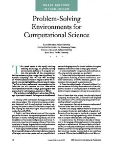
3.3 Solution of reactor simulation. : : : : : : : : : : : : : : : : : : : : : : :
78
3.4 Modeling drying and shrinkage of salami. (A) shows the initial model with R being the radius of the \inside" of the salami and with d being the radius of the casing. (The gure greatly exaggerates d; generally d 6, end{e�ects have been neglected and the transport of heat and mass was assumed to occur in the radial direction only. It was also supposed that mass transfer in the rod occurs in liquid form and has no in uence on the heat transfer inside the material. The heat capacity in the casing has been neglected.
78
Figure 3.3 Solution of reactor simulation.
79
R
d
R
d
R
d
(1)
(2) (3)
(A)
(B)
(C)
Figure 3.4 Modeling drying and shrinkage of salami. (A) shows the initial model with R being the radius of the \inside" of the salami and with d being the radius of the casing. (The gure greatly exaggerates d; generally d