Proceedings of the ASME 2012 International Design Engineering Technical Conferences & Computers and Information in Engineering Conference IDETC/CIE 2012 August 12-15, 2012, Chicago, IL, USA
DETC2012-70406
A GRAPH GRAMMAR BASED APPROACH TO AUTOMATED MANUFACTURING PLANNING Wentao Fu Automated Design Lab Department of Mechanical Engineering The University of Texas at Austin Austin, Texas 78712 Email:
[email protected] Pradeep Radhakrishnan Automated Design Lab Department of Mechanical Engineering The University of Texas at Austin Austin, Texas 78712 Email:
[email protected]
Ata A. Eftekharian Automated Design Lab Department of Mechanical Engineering The University of Texas at Austin Austin, Texas 78712 Email:
[email protected]
Matthew I. Campbell* Automated Design Lab Department of Mechanical Engineering The University of Texas at Austin Austin, Texas 78712 E-mail:
[email protected]
ABSTRACT In this paper, a new graph grammar representation is proposed to reason about the manufacturability of solid models. The knowledge captured in the graph grammar rules serves as a virtual machinist in its ability to recognize arbitrary geometries and match them to various machine operations. Firstly, a given part is decomposed into multiple sub-volumes, where each sub-volume is assumed to be machined in one operation or to be non-machinable. The decomposed part is converted into a graph so that graph grammar rules can determine the machining details. For each operation, rules determine the face on the part that the tool enters, the type of tools used, the type of machine used, and how the part is fixed within the machine. A candidate plan is a feasible sequence of all of the necessary machining operations needed to manufacture this part. If a given geometry is not machinable, the rules will fail to find operations for all of the partitions. As a result of this representation, designers can quickly get insights into how a part can be made and how it can be
Christian Fritz Palo Alto Research Center Intelligent Systems Laboratory Automation for Engineered Systems Palo Alto, CA 94304 E-mail:
[email protected]
improved (e.g. change features to reduce time and cost). A variety of tests of this algorithm on both simple and complex engineering parts show its effectiveness and efficiency. 1.
INTRODUCTION In order to better streamline the interaction between the mechanical design process and manufacturing, an approach is being developed which automatically reasons about CAD model to define detailed and optimal manufacturing plans. The larger system is known as AMFA: Automated Manufacturing Feedback Analysis (AMFA), and this paper presents the graph grammar based representation scheme that serves as the system’s foundation. Starting from a CAD model provided by the designers, the grammar representation scheme performs an analysis of manufacturability on it by referencing the data provided on the manufacturing facility that will build the part in question. The outputs of AMFA are potential manufacturing plans, their associated times and costs, and, in certain cases, recommendation on how to change the part so that it is more easily manufactured.
* Corresponding Author, Phone: (512) 232-9122, Fax: (512) 471-6356, email:
[email protected] Approved for Public Release, Distribution Unlimited. Copyright © 2012 by ASME
Original part
Convex decomposition
Bounding box
Removal volume
Seed graph
Grammar Representation
Search tree during reasoning process
Figure 1. Flowchart of the Representation Scheme
To generate the outputs, two distinct areas of efforts are involved in the representation scheme. They are summarized into the Convex Decomposition and the Grammar Representation as shown in Figure 1. Firstly, a new method of decomposing 3D solid models was developed, which is indicated in the upper portion of Figure 1. To begin with, a CAD model in the STEP format 1 (Part A in Figure 1) provided by designers is loaded into the tool. Then this geometry – comprised of vertices, edges, and faces – is parsed into a label-rich graph which serves as the basis for the representation (the lower portion in Figure 1). In the translation, a bounding box (Part B in Figure 1) is extrapolated from the original part A since one would likely start the actual manufacturing from a larger block of material. The original part A is then subtracted from the bounding box to create the 1 .STEP is used as the standard format for the exchange and conversion of solid models
Approved for Public Release, Distribution Unlimited.
removal volume (Part C in Figure 1) that is to be removed. This removal volume then undergoes further divisions to generate compact sub-volumes where each sub-volume is assumed to be machined in one operation or to be nonmanufacturable. The decomposed removal volume is then converted into a graph and used as the initial seed in the representation. The grammar representation reasons about the manufacturability of a given part under certain foundry capabilities. Firstly, all available manufacturing processes within a foundry are translated into grammar rules. The rules are then organized to reason about the seed graph in order to determine its machining details. A search tree is drawn to describe how they work on the seed graph. Steps in the tree represent alternative manufacturing operations for different sub-volumes. These operations are determined through the rules which detect a series of graph elements and relate them to a particular manufacturing process. Each operation consists of the tool entry face, the tool type choice, the machine choice, and the needed fixture to machine one sub-volume. As the tree grows, more and more sub-volumes get manufactured. When the tree propagates to its bottom, there are no more subvolumes of the given part to be machined, and a complete search space that includes all alternative manufacturing plans for the given part is derived. In addition, by translating foundry capabilities into graph grammar rules, a precise conclusion of non-manufacturability of a part can be made if the rules fail to find a manufacturing plan for a part. It signals that the manufacturing process is beyond the foundry capability and this part needs to be redesigned. This paper describes the grammar representation and shows how the method functions on a few test parts. In the next section the relevant research is described and how it compares to this project (Section 2). This is followed by a description of how the STEP file is converted into the seed graph for use in the Grammar Representation (Section 3). Sections 4 and 5 present the seed format and the rules that reason with the graph. In Section 6, a tree search algorithm is described which used the representation. The paper closes with examples and discussion (Section 7) and a conclusion and future work section (Section 8). RELATED WORK Automated manufacturing planning was first proposed by Russel [1] in 1967. Due to the fast development of Computer-Aided Process Planning (CAPP) since the 1980s, this topic continues to receive much attention both from researchers and practitioners [2]. In this time, many knowledge based approaches [3, 4, 5] were developed to capture the basic logic used by a process planner. Marri, Gunasekaran and Grieve [2] provided a comprehensive review of these CAPP based systems. Based on their conclusions, more attention should be paid to the architecture and constraints for machining operations while developing a CAPP system. More recently, Sharma and Gao [6] proposed a process planning system using the latest tools and technologies and to fully comply with the international standard for exchange of product data, but it is only intended for simple prismatic parts and the feedback analysis cannot be 2.
2
Copyright © 2012 by ASME
automatically imported into CAD systems for detailed redesign. Allen et al. [7] developed an agent-based approach that can provide a number of generic solutions whilst maintaining the ability for manual intervention to establish local working preferences, but the efficiency of this algorithm is restricted by its parametric optimization process. In contrast, the graph grammar based approach to automated manufacturing planning considers a large variety of topologies rather than being restricted by the optimization process. It utilizes a technique of creating new graphs from an original graph (host) by applying prescribed rules onto the host [8]. The rules are of the form LR where the left hand side (LHS) includes elements and conditions to be recognized and satisfied in the host graph and the right hand side (RHS) indicates the transformations of those elements that have been recognized in the host. A widely used grammar based approach in automated manufacturing planning is Form-Feature Recognition (FFR) technique [9]. This is primarily important because it can extract or generate higher level and meaningful geometric entities that are not easily inferable from the solid geometry. These geometric features can serve as a bridge between the geometry on one hand and manufacturing reasoning on the other hand which is a crucial step in computer-aided part design [9]. A thorough survey of various techniques in FormFeature Recognition can be found in the work by Han [10], Shah [11, 12], and Subrahmanyam [13]. According to these surveys, three dominant techniques which include graph, volumetric and hint based approaches are mostly used in modern FFR algorithms. Graph based techniques, although proven to be reliable in recognizing isolated features, suffer from the complexity of the geometry and the fact that features may have interactions with each other [14, 15]. Some researchers [16] have tried to tackle the problem by introducing various types of heuristics to the algorithm and have gained considerable achievements but still the problem remains unsolved for complex geometries. Others [14, 17] have tried to add missing elements that correspond to interacting features into the graph but despite the added complexity they do not completely solve the problem. Volumetric decomposition methods stand apart from the others, both in the algorithm employed and the results. Researchers have continued to extend and refine this approach to solve numerous shortcomings, such as non-convergence and geometric domain restrictions. The volumetric decomposition method can handle interactions and provide additional information such as geometry-based precedence relations [18]. A very similar approach to that proposed in this paper was provided by Ertelt and Shea [19]. Knowledge of fundamental machine capabilities was encoded by generating a vocabulary of removal volume shapes based on the available tool set and machine tool motions. Since this method coupled the topological representation and parametric evaluation process together, its scalability to complex parts and nontraditional machined parts is questionable.
simple removal volumes from the work-piece. These topological entities are commonly referred to as machining features in literature. In this work we extend the idea beyond the volumetric decomposition approach for 3D solid models by adding a layer of reasoning to the algorithm. Our decomposition algorithm [20] uses a ranking strategy to prioritize concave-edges, which define the division and three heuristics to evaluate the direction of cut for each division. Results of convex decomposition can be represented as a tree structure with branching factor equal or greater than 4 (4 is the case when there are exactly two solids generated after each cut) and depth of the tree equal to the total number of concave edges in the solid.) . Each node represents a volume that needs to be cut and each branch represents a left (L) or right (R) cut in the tree. Each nodes consists of either a simple shapes (i.e. a convex volume) which is represented as an (S) in the tree or a complex shape (i.e. a volume with one or more concavities) which is represented as a (C) in Figure 2. For a given solid model as shown on the top of Figure 2, let us consider a case where the left branch is always chosen as the preferred cut, and the result after first cut is one complex (C) volume and one simple (S) volume. The simple volume does not need any further cutting operations so the branch related to this node stops here; this is shown as a red node in the tree. For each complex volume (C) the branch grows further to lower levels until it hits a simple volume (S). In order to find the best result (or an optimal decomposed solid for the representation) one can generate all the possible options in the tree and explore and evaluate each individual option from the pool of solutions. This, however, is not a good idea due to the fact that Boolean operations are computationally expensive and slow in CAD kernels. Furthermore evaluation conceptually requires a human to
3.
CONVEX DECOMPOSITION In the context of computer-aided manufacturing, convex decomposition is primarily important and useful for generating
Approved for Public Release, Distribution Unlimited.
Figure 2. Convex Decomposition Tree
3
Copyright © 2012 by ASME
inspect the result and decide if it is a good decomposition or not (computationally evaluating the quality may be possible, but it is out of the scope of the work). Therefore, it is nearly impossible to explore all the options or branches in the tree. The alternative solution is to expand a single but promising branch. At each level in the tree the algorithm evaluates the solutions and decides the preferred direction for the next level. This continues until no more complex volumes are detected. In order to reach this goal, two sets of heuristics are designed and implemented to guide the convex decomposition algorithm along the desired direction. It is important to note that a desired solution is described as a decomposed volume that contains partitions which are suitable for manufacturing purposes. In other words, all the sub-convex-volumes should possess certain properties which include (1) having a compact shape with no or few number of concavities, (2) having a prismatic or close to prismatic geometry. Due to the lack of space, details about the algorithm, the procedure for cutting the solid and evaluating each cut are omitted here and we refer the interest reader to [20]. Based on the designed heuristics, only desirable branches will survive and continue to grow until no further volumes of type C are recognized by the algorithm. The final decomposed shape is a combination of remaining S type volumes in all traversed branches. The candidate decomposed solid at the bottom of Figure 2 is a sample result after the heuristic-guided convex decomposition. SEED LEXICON After the removal volume of a given solid model is decomposed, the compound solid comprised of different subvolumes has to be translated into a seed graph such that the grammar representation can work on it. Rather than using existing graph techniques to represent a solid model, a new lexicon is proposed. Figure 3 gives an example showing that how a solid model shown as part A in Figure 1, is described as a label-rich graph.
This example is a simple shape with a pocket in front and a through hole in the back. In this graph, geometric elements are described by nodes, arcs, and hyperarcs. Nodes are used to represent vertices and faces. Arcs are used to represent edges in the shape as well as to indicate relative positioning information (parallel, perpendicular, etc.) between any two faces. A hyperarc is a special arc. While arcs can only connect two nodes, a hyperarc can connect as many nodes as needed. It is always used to connect all vertices belonging to a face to their face node. Figure 4 gives an example of a complete representation for a face with four vertices in the seed lexicon. The node n0 with label “face” represents the face and the other four nodes with label “neg_vertex” represent all the vertices. They are connected by hyperarc ha0, which also has a label “face”. This label is to distinguish this hyperarc as a face hyperarc from the other types of hyperarcs used in the lexicon.
4.
Figure 3. The simple solid model shown as part A in Figure 1 as a seed graph in representation
Approved for Public Release, Distribution Unlimited.
Figure 4. A sample face representation in the seed lexicon
Another type of hyperarc is defined to encompass a subvolume by connecting all of the nodes of a sub-volume together. For example, in Figure 3, the hole and the bottom cuboid are separated by two green hyperarcs. By using nodes, arcs, and hyperarcs in the seed graph, all geometric information about vertices, edges and faces for a solid model is stored. In this way, face nodes are used in the seed and rules to refer to general machining features, like holes, pockets and slots. Moreover, edges and vertices provide more details about shapes and geometries, which are necessary for the rules to describe manufacturing operations more precisely. It is also important to note the variety of labels in the graph, which are used to store topological, rather than parametric, information. A face node may have label “bb”, which indicates that this face is a bounding box face. If a face node represents a face belonging to the removal volume, it will have the label “neg”. For example, in Figure 3, the face node n1 (not explicitly shown, but overlaps with its face hyperarc ha1), which represents the bottom face of the cuboid, has label “neg”, while face node, n12, has label “bb. A hyperarc may have label “original”, which means the face this hyperarc connects to is an accessible face to the tool and it is a candidate face for the tool entry face selection. Examples include the hyperarc ha1 and ha9 in Figure 3 and ha0 in Figure 4. Besides, the face adjacency property, either “convexity” or “concavity”, between any two adjacent faces is stored in the label of their common edge. With these labels, the rules can do a much more precise reasoning about the graph elements they
4
Copyright © 2012 by ASME
capture and the search can be more successful. The detailed explanation of the rules based upon the label-rich seed graph is given in section 5. 5.
RULE DEVELOPMENT With an understanding of how a compound solid model comprised of different sub-volumes for a given part is represented in the seed, it becomes easier to tell how the rules are developed. In this part, eight sets of graph grammar rules have been devised to simulate a virtual machining process, removing material of the compound solid step by step. This process will end if the volume of the compound solid becomes zero. These rule sets are arranged in a specific sequence such that they collectively perform the required reasoning as a whole. The first rule set (rule set 0), the “pre-processing” rule set, aims to recognize typical sub-volumes (counter-sink, round edge, etc.) and non-traditional machining operations (bending, etc.) which are tagged for later use. These subvolumes are usually machined in a finishing process using specific tools. By recognizing and isolating these special cases at the first stage, more realistic manufacturing plans which separate roughing and finishing processes can be generated. Unlike other machining operations, bending operations do not remove material. They simply change the shape of the seed graph. However, this change does affect the generation of a correct bounding box for a given part. In this case, the rules in this rule set operate in cooperation with the Convex Decomposition to implement these non-material-removal operations on the part before a correct bounding box is generated. The second and third rule sets (rule set 1 and 2) are used to identify a feasible tool entry face on a sub-volume that is to be machined. Firstly, in rule set 1, a single rule is designed to capture a face which is accessible by the tool. If such a face is found, it will be labeled with “machining_start”. If no faces are found, the process terminates – there are no sections left to machine.. In rule set 2, there are two rules, representing two special cases, where a tool entry face selected from rule set 1 needs to be rechecked. For example, an accessible face is not allowed to be chosen as a tool entry face if a sub-volume could not be fully removed from this face. An infeasible tool
internal circular face of the hole that is shared by the front pocket becomes accessible to the tool. But this face is not a good choice of the tool entry face since from this face the tool cannot access the whole material of the pocket. Despite being a valid face to begin machining in rule set 1, the choice is invalidated in rule set 2. After rule set 1 and 2, a feasible tool entry face has been identified. Then, the representation goes to rule set 3, which is responsible for tool type selection. Rule set 3 is a cluster of available tooling operations, including Drilling, Milling (End Milling and Ball Milling), Sheet Cutting (Water Jet), and Counter-sinking. Each tooling operation corresponds to one or more rules in this rule set. These rules are specially designed based on how each operation is implemented. For example, in this rule set there are two drilling rules as shown in Figure 6. The reason for creating two rules is that there are two different representations for holes in STEP files. The planar circular face of a hole can be represented with either two vertices and two semi-circular edges (type 1) or one vertex and one circular edge (type 2). Figure 6(a) recognizes the first hole type. The LHS of this rule finds a hole to be machined by capturing its cylindrical face (a hyperarc labeled with “cylinder”) and one of its planar faces, which is accessible by the tool and is depicted as another hyperarc labeled with “machining_start”. Additionally, since this hole is also a sub-volume to be machined, its sub-volume hyperac (a hyperarc with label “convex_shape”) is also captured. If such a hole is found, a drilling operation is implemented on this sub-volume, which is described by a virtual transformation from LHS to RHS of the rule. After that, this sub-volume’s machining_start face and its sub-volume hyperarc become “machined”. Similarly, Figure 6(b) is the drilling rule for the hole of type 2.
(a) Drilling rule 1 for hole of type 1
(b) Drilling rule 2 for hole of type 2 Figure 6. Screenshots of two drilling rules in GraphSynth Figure 5. An example of infeasible tool entry face
entry face is described in Figure 5 using the same solid model as discussed in Figure 3. If the hole is first removed, the
Approved for Public Release, Distribution Unlimited.
Similar algebraic reasoning is performed for the remaining tool types where complete Left Hand Sides have
5
Copyright © 2012 by ASME
been developed to capture the intricacies of the geometric constraints. After a tooling rule has been selected and applied to a sub-volume, this sub-volume is marked as machined. Then the representation moves to rule set 4, which is a “post-processing” rule set. This set generally takes care of any remaining issues regarding label changes and graph modifications after each tooling operation. For example, a very often recognized rule in this rule set is used to delete any remaining faces which realistically should have been removed after a previous tooling operation. Once a complete tooling operation is finished after rule set 4, the corresponding fixture method and machine type used to conduct this tooling operation are selected in rule set 5. Currently these two decisions are made in one single rule by considering which bounding box face to fix and the relative positioning relation between the fixed face and tool entry face of this sub-volume. If they are parallel, then a VMC, or Vertical Machining Center, is chosen. If they are perpendicular, a HMC, or Horizontal Machining Center, is recognized. The rule for the VMC is shown in Figure 7. The LHS of this rule captures a pair of parallel faces while one face is a bounding box face (the face node n2 labeled with “face” and “bb”) amd the other face is a tool entry face (n1 labeled with “face”, “neg” and “machining_start”). If these two faces are found, then the bounding box face n2 will be “fixed” and the “VMC” will be chosen. Future endeavors for this rule set are focusing on extending machine types to multiaxis machines such that more general fixtures can be covered. After fixture design and machine type selection, the following rule sets 6 and 7 are “post-processing” rule sets. Similar to rule set 4, they are doing some clean-up, like adding new “original” labels to those faces which become exposed to the tool after certain sub-volumes have been removed. After rule sets 6 and 7, one complete step in a manufacturing plan has been defined to machine current subvolume. Then the representation will go back to rule set 1 to start another loop for another sub-volume. This representation
Start
No
Rule set 0 (Preprocessing rule set): loop until no rules recognized
Rule Applied?
Figure 7. The VMC rule from Rule set #5 in the grammar representation
loop is shown in Figure 8. If all the sub-volumes for a given part are machinable, the similar loop for each sub-volume will continue until all sub-volumes are machined. At that time, since there are no more tool entry faces for rule set 1 to choose, the looping process will terminate with a complete manufacturing plan for the part, which we refer to as a goal in the search tree. However, as seen in Figure 8, rather than finding a complete machining recipe, the reasoning process can also end at different stopping points defined by different rule sets. Depending on the function each rule set performs, the representation loop ends at these stop points either when there is no rule applied in certain rule sets (rule sets 3 and 5), or when a particular termination rule is recognized (rule set 2). For the first scenario, for example, the looping process will stop if there is no tooling rule in the Tool Selection rule set that is recognized for a sub-volume. If this case happens, the user can gain an insight that a current sub-volume of a given part is actually not manufacturable with current available tooling operations described in the Tool Selection rule set. Since a foundry’s capability is always mapped into different tooling rules, it is equivalent to conclude that the manufacturing of this part is beyond given foundry’s capabilities. One can either redesign the part to make it easier to manufacture, or one can import more advanced machines
No
Rule set 1 (ChooseStartFace): maximum 1 rule application
Rule set 3 (Tool Selection): maximum 1 rule application
Rule Applied? Yes
No
Rule Applied?
Goal (Recipe found) Yes
Rule set 7 (Post_processing_3) : maximum 1 rule application
Rule set 2 (StartFaceCheck): maximum 1 rule application
Yes
Stop
Rule set 4 (Postprocessing_1): loop until no rules recognized
Rule set 5 (Base MachineSelection): maximum 1 rule application
Rule Applied?
Yes
Rule set 6 (Post_processing_2) : loop until no rules recognized
No Figure 8. Flowchart of rule sets
Approved for Public Release, Distribution Unlimited.
6
Copyright © 2012 by ASME
and tools into the foundry to cover required tooling operations. For the second scenario, for example, the rules in rule set 2 define several infeasible cases of tool entry face selection. If any rule in rule set 2 is invoked, the tool entry face selected in rule set 1 becomes invalidated, and the search will terminate after this rule has been applied. Therefore, depending on the given part and the knowledge of the manufacturability analysis built in the rules, a complete looping process described in Figure 8 will either find a feasible manufacturing plan, or converge on no plan. One should be aware that this complete reasoning process only represents one branch in the search tree in Figure 1. The whole search process actually contains numerous branches where each branch is depicted as one complete looping process in Figure 8. More detailed discussion about the search tree is given in next. 6.
TREE SEARCH ALGORITHM Now that the seed graph and all necessary rules have been described, a search process using these rules is presented which seeks feasible and optimal manufacturing plans. A graph grammar based software tool called GraphSynth [21] previously developed by the research team is used as a platform where the seed graph can be loaded and a RecognizeChoose-Apply cycle is invoked to define the tree. During the search a candidate host graph is provided to a Recognition procedure which checks all the rules within a single rule set to find valid rules that can successfully change the graph. This defines a list of options which are essentially different branches in a search tree (similar to Figure 1). Amongst these options, one is chosen. However, given the expanse of computer memory most tree-search algorithms choose all possible paths thus defining a population of states. The Apply procedure executes the L-to-R graph transformation algebra to change the host state into a new graph. In several of the rule sets described in section 5 (0, 2, 4, 6, and 7), the options do not define meaningful alternatives paths. The rules within these rule sets simply prepare, fix, or check qualities of the graph. Many of the resulting options are confluent which means that they result in graph changes which do not negate other options from being called. As such these rule sets do not define alternative decisions in the tree. However, the decision rule sets (1, 3, and 5) create decisions based on (1) the tool entry face where machining is initiated, (3) the choice of tool to use, and (5) the type of machine and fixture orientation to use. Various blind and guided search algorithms have been applied to this grammar representation. In this paper, a depthfirst search is shown which exhaustively defines all possible plans for a given part. This is done to validate the feasibility and completeness of the design space. In order to better guide the search to a single best solution or a set of best solutions, some measure of the quality of a particular operation or a manufacturing plan (i.e. a set of operations) is necessary. This evaluation method is shown in [22] and discussed briefly in Section 8.
7.
EXAMPLES AND DISCUSSION The current grammar representation has been tested on over 25 solid models, ranging from self-designed simple geometries to complex suspension components provided by the military contractors. In this section, three examples are provided to illustrate the manufacturability analysis capability of the representation, including one easy part (the shape shown as part A in Figure 1), one real part, which is a chassis part for small vehicle (Figure 11), and one complex part, which is also a component assembled in a small vehicle and is referred to as “radio box” (Figure 13). For the simple example, the generated search space that consists of all the feasible manufacturing plans will be verified. For the main chassis and the radio box, selected recipes for these parts and the underlying characteristics of the representation tool will be explained. This section ends with a comparative case study of a non-manufacturable part using the representation tool and the commercial software, FeatureCAM [23]. The results show our technique’s expertise in instantly generating nonmanufacturability feedbacks for a given part and effectively communicating them to the end users. 7.1. Manufacturability Analysis For the simple part, one may easily come up with a manufacturing plan. One such plan may be to first remove the bottom cuboid from the bottom face ha1 (as indicated in Figure 3), then drill the top hole from face ha7. In this way, only one fixture is needed. However, in a complete search tree created by automatically employing the rules on this seed graph, this plan is only one branch. All other branches representing different alternative plans are simultaneously generated. One sample plan is shown in Figure 9. In this manufacturing plan, the upper portion is a stepby-step description of how the rules were implemented. An executable machining plan was provided at the end. Based upon this recipe, two steps are needed to make the part. The first step is to fix the bottom face and drill the top hole from its top surface. A VMC is needed to finish this operation. Then the part is flipped over and the top face is fixed. The remaining cuboid is end milled from its bottom surface. Of the
Figure 9. A sample manufacturing plan for the solid model shown as part A in Figure 1
Approved for Public Release, Distribution Unlimited.
7
Copyright © 2012 by ASME
96 valid plans that are found (as discussed next), there are several inefficient plans like this one, and several of the more likely single-fixture approach. Figure 10 is a summary report after all possible manufacturing plans have been found. Within 2 seconds 96 solutions were generated for this simple part. The completeness is reflected by the total nodes in the search tree while the efficiency is reflected by the search rate, i.e. Nodes/Sec. One may doubt the large size of solutions. However, this number can actually be verified by a pure mathematical derivation.
(a) Original main chassis part
Figure 10. Summary report of the search space for the part discussed in Figure 8
If starting from ha1, only the End Milling tool is capable of removing the bottom cuboid. Despite the three bounding box faces that are coplanar with the outer surface of this cuboid where machining will happen, there are three other faces available for fixturing. After removing the cuboid, the hole can be either drilled or end milled from either its top face or its inner planar face. For the first case, there are five kinds of fixture, and for the latter one, there are six. So in total, ( ) solutions are found. However, the upper face, ha9 can also be chosen as the first entry face. Both End Milling tool and drill bit can be used to remove the hole. Five bounding box faces are available for fixture. After the hole, the cuboid can only be End Milled from ha1 with three different fixtures. So another solutions are found. Therefore, in total 96 candidate plans are derived, exactly the same number of solutions found by the software. This example shows the validity of the grammar representation scheme. The grammar rules are good at creating a complete search space, which covers all possible and realistic candidate manufacturing plans for a given part, while the geometric reasoning about feature interactions is properly conducted by a specially designed search sequence for the rule sets. Another example given is a main chassis part for a small autonomous vehicle (Figure 11). This part is unique due to its inclined tip, one rectangular through pocket and countersinked holes. Apparently, it is manufactured from sheet metal with final bending operations. In addition, non-traditional machining operations are needed to cut out sharp corners for the pocket. For simplicity, some duplicate holes and triangular pockets were removed. However, even the simplified part (Figure 11(b)) has 12 sub-volumes, which represent at least 12 steps to machine this part. Due to the complexity, the seed graph converted from the simplified model is not shown. For this part, the preferred manufacturing plan is to first cut out the sheet metal with exactly the same shape, then either machine the holes or cut off the pockets, after that machine all countersinks continuously, and finally do several bending operations. However, since the software first looks at the final part then does a backward reasoning of how it was
Approved for Public Release, Distribution Unlimited.
(b) Simplified main chassis part Figure 11. Main chassis part
machined, one may expect that bending operations, instead of being the last few operations, are actually replaced by unbending operations at the very beginning of a generated manufacturing plan. For the same reason, the seed graph used in this case was not converted from the simplified part. As mentioned in section 4, rather than removing material, bending operations significantly change the shape of a given part. As a result, the right bounding box and negative part could not be generated from that simplified part (Figure 11(b)). To solve this problem, a special heuristic is designed in the Convex Decomposition such that once a bending operation is detected for a given part, all needed pre-unbending operations are executed in the convex decomposition first, then the unbent part is used to generate the seed graph. In this case, the seed graph was converted from a sheet metal part which has already been unbent from the simplified main chassis part. A sample recipe is shown in Figure 12.
Figure 12. A sample manufacturing plan for Chassis part
From the recipe one can see that actually five unbending operations are needed before machining process starts. After that, the Water Jet is used to cut most of the sub-volumes. It is very important to note that counter sink operation always goes after drilling operation to satisfy the manufacturing constraint that there is no hole before the hole is drilled. The complete search space of all possible manufacturing plans for this part expands exponentially as the total number of sub-volumes increases. For the simplified part with 12 subvolumes (Figure 11(b)), an estimation of the size of the search
8
Copyright © 2012 by ASME
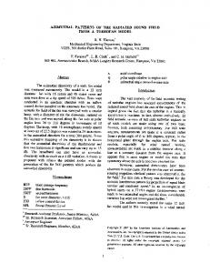
space is conducted from the fact that there are at least one tool entry face, two fixtures and machine types and three tooling operations available, which in total represents 6 different options, for each sub-volume to choose. Moreover, these 12 sub-volumes can be manufactured in a random order. Therefore, in total at least trillion solutions are included in the search space. This underscores the need for an approach to eliminate many of these solutions to focus on more beneficial solutions. An ongoing evaluation research for the optimization of the search space generated in the representation is discussed in next and the details are given by Blarigan, et al [22]. In the third example, the “radio box” solid model is given to illustrate the representation tool’s capability of extracting sub-volumes from the interacting regions in the solid using specially designed heuristics. From Figure 13 (a) we can see that on the right hand side of this part, there is a complex region (shown in a dashed box), which is an interaction of a vertical hole, a front hole and a cylindrical shape in the middle (as indicated by arrows). The negative shape for this region is indicated in Figure 13 (b). Starting from this negative shape, our tool first detects all the features in this region by reasoning about the properties of the negative geometric elements, like the curved edges and the cylindrical faces. Then the heuristics guide the convex decomposition to cut the region such that the most complete features are recovered. After that, the remaining material in this region is further decomposed based upon the other features that are detected. Eventually the convex decomposition will decompose the interacting region into multiple sub-volumes. Each sub-volume represents a separate feature extracted from the region. More details about the heuristics in the convex decomposition are given in [20]. The middle cylinder
The vertical hole
volume B is the negative of the front hole; and the sub-volume A is the negative of the middle cylinder. The convex decomposition correctly determines that the vertical hole (the sub-volume C) is the most complete feature to recover. This tells the representation that a drilling or a milling operation is needed to remove this sub-volume. Moreover, the front hole is partially recovered as the sub-volume B. Although this is not a complete feature, its semi-circular front face and the partial cylindrical face provide enough information to inform the representation that another drilling or milling operation is needed to machine this sub-volume. As for the sub-volume A, it consists of all the remaining negative material for the interacting region. Since this sub-volume is prismatic, the representation tool always calls the milling tool to remove it. Overall, based on the number of features detected, a feasible sequence of manufacturing steps that are needed to remove the entire interacting region is generated. Similarly, the representation implements the reasoning process for the interacting region on the left as well as the other sub-volumes of the radio box. A complete manufacturing plan is provided in Figure 14. In this plan, step 17 removes the sub-volume A; the sub-volume B is removed in step 20, and step 22 removes the sub-volume C. As discussed above, the convex decomposition is able to recognize all features and generate individual sub-volumes for each feature in an interacting region. However, one should note that the sub-volume for each feature might not be fully recovered. This is due to nature of interacting regions: by removing one feature’s sub-volume, the other features’ subvolumes will be unavoidably damaged. However, the partially recovered sub-volumes provide enough information, including geometric elements (e.g.: circular edges, counter-sinks) and their properties, to inform the representation correctly what features the sub-volumes represent and the manufacturing details for these sub-volumes. The heuristics implemented in our tool to deal with the interacting machining regions also has a beneficial side effect. By recovering the most complete features first, it simulates a
The front hole (a) The original part of radio box A: the negative of middle cylinder B: the negative of the front hole C: the negative of the vertical hole (b) The decomposed compound negative solid of the radibo box Figure 13. The solid model of radio box
For this radio box case, the final decomposed volumes for the interacting region are shown in Figure 13 (b). The subvolume C is the negative shape of the vertical hole; the sub-
Approved for Public Release, Distribution Unlimited.
Figure 14. A sample manufacturing plan for the radio box
9
Copyright © 2012 by ASME
roughing manufacturing process in the foundry, which is used to remove as much material as possible in the first few operations. The following operations for the remaining small or partial features generated in the representation tool constitute a finishing process. More precise tooling operations are needed in order to satisfy the high tolerancing requirements that are associated with the positive part. As a result, less material is expected to be removed. It is also important to be aware that in this manufacturing plan most of the sub-volumes are removed by the same type of tool. Even for the sub-volume C, instead of using a drilling tool, an end milling tool is called to remove this sub-volume. The advantage of minimizing the types of tools needed in one manufacturing plan is that the manufacturing time and cost can be reduced. Without changing the tools, many refixtures become unnecessary and the manufacturing process becomes more continuous and faster. Additionally, given the fact that the milling tool is more efficient than the drilling tool in terms of removing a large amount of material, the milling tool is always preferred in the current representation as long as the tolerance requirements for each sub-volume are satisfied. 7.2. Non-Manufacturability Analysis The non-manufacturability of a given part is due to two constraints. One is the foundry capability limitations and the other is the flaws in the designer’s model. The nonmanufacturability analysis in the representation is implemented by the rules through the topological, rather than parametric, reasoning processes. At this stage, we intentionally relax the parametric constraints imposed by the foundry limitations. One reason is that these constraints, such as the lack of appropriate size of tool, can always be solved by importing needed tools into the foundry. Thus, no redesign feedback for the designers is needed. However, the design flaws detected by the representation tool usually relate to the topological defects in the given part. The underlying logic in the representation is that if a part is topologically not manufacturable because of: 1) inaccessible regions in this part (for example, the inner sharp corners in part in Figure 15); 2) geometric defects in the given solid model; 3) unrecognized or invalid geometric elements (for example, an edge with more than two vertices); etc., then this part would always be nonmanufacturable unless required redesign modifications is made by the users.
For instance, consider the part in Figure 15. It is not manufacturability due to an inaccessible sharp edge from either tool feed direction. From the analysis report shown in Figure 16, we see that the representation tool asserts that no manufacturing plan can be found for this part in almost no time. Additionally, the user is informed that all the inner sharp edges should be removed before the part can be machined. This example shows how our tool communicates with the user instantaneously in terms of design improvements.
Figure 16. A sample manufacturing plan generated from the representation for the part in Figure 15
The same part has also been checked in FeatureCAM. To compare, FeatureCAM proposed a manufacturing plan as shown in Figure 17.
Figure 17. A sample manufacturing plan generated from FeatureCAM for part A in Figure 15
In this plan, we see that due to the sharp edges, two rounds of rough and finish passes were employed to remove the negative cuboid. However, no matter how high the manufacturing precision that the tool can achieve, the sharp edges would never be created exactly as how they were designed. Figure 18 indicates the artifacts left in the final shape after the manufacturing plan has been implemented. These areas are actually where the non-manufacturable sharp edges are located. Rather than trying to tackle the bad geometries by the ineffective employment of the foundry capability, our representation tool returns the redesign suggestions directly to the user in a much earlier phase. This feature distinguishes the representation tool as a user-centric effective non-manufacturability feedback provider.
Figure 15. A non-manufacturable part due to design flaws
Approved for Public Release, Distribution Unlimited.
10
Copyright © 2012 by ASME
The inaccessible chips after manufacturing
Figure 18. The comparison between the original part in Figure 15 and the solid machined in FeatureCAM
8.
CONCLUSION AND FUTURE WORK This paper describes a graph grammar based approach to reasoning about the manufacturability of given solid models. A two-module structure of this approach separates the geometric conversion of a solid model, which is done in the convex decomposition, and the topological reasoning of manufacturability, which is realized in the representation. While the convex decomposition is mainly used to decompose a model into multiple sub-volumes, which serve as the basis for the representation, it can also take advantage of the numerous functionalities built in Open CASCADE to preprocess some complex parts, as in the second example that unbends a part as required. In this way, more realistic manufacturing plans can be generated. On the representation side, a topological reasoning process for a solid model is realized using the seed lexicon and graph grammar based rules. By storing all geometric elements and topological relations of a solid model in the seed lexicon through nodes, arcs, hyperarcs and labels, the generic nature of the representation scheme is ensured. The completeness and validity of the representation are realized by the rules and a specially designed search sequence for the rule sets. However, it is not enough to only have a large number of automatically generated manufacturing plans. A continuing effort in evaluating these plans and deciding the optimal one based on user-specified objective functions is occurring. To implement this effort, a more detailed evaluation and optimization process is being developed. The output of the representation, including the tool type, machine type, fixture for each operation in a manufacturing plan, is used to evaluate each plan. The search process then makes a decision amongst these evaluated plans. The goal is to find the optimal manufacturing plans. This work has been presented in detail by Blarigan, et al [22]. Another research effort currently in progress is to extend tooling operations and machine types to turning centers (i.e. lathe) and multi-axis milling centers. For complex parts, a user
Approved for Public Release, Distribution Unlimited.
may prefer a manufacturing plan with few steps which can be implemented in a multi-axis milling center rather than a manufacturing plan that is decomposed into lots of sub-steps and can be implemented with a 3-axis milling machine. More non-cutting machining and tooling operations need to be translated into rules to handle such complexities. With an ongoing cooperation with the evaluation and optimization and a continuous work on expanding the capability of the representation scheme, an intelligent graph grammar based tool, which not only provides design insights in terms of manufacturability to the designers, but also outputs optimal manufacturing plans to the engineers, is close to becoming a reality. ACKNOWLEDGEMENT This material is based upon work supported by the Defense Advanced Research Projects Agency under contract FA8650-11-C-7130. The views expressed are those of the author and do not reflect the official policy or position of the Department of Defense or the U.S. Government. REFERENCES [1] E. L. Russell, Automated manufacturing planning, New York: American Management Association, 1967. [2] H. B. Marri, A. Gunasekaran and R. J. Grieve, "Computer-Aided Process Planning: A State of Art," The International Journal of Advanced Manufacturing Technology, vol. 14, 1998. [3] H. R. Berenji and B. Khoshnevis, "Use of artificial intelligence in automated process planning," vol. 5, no. 2, 1986. [4] G. Chryssolouris and S. Chan, "An Integrated Approach to Process Planning and Scheduling," Annals of the CIRP, vol. 34, no. 1, 1985. [5] H.-p. Wang and R. A. Wysk, "A knowledge-based approach for automated process planning," International Journal of Production Research, vol. 26, 1988. [6] R. Sharma and J. Gao, "Implementation of step 224 in an automated manufacturing planning system," 2002. [7] R. D. Allen, J. A. Harding and S. T. Newman, "The application of STEP-NC using agent-based process planning," vol. 43, pp. 655-670, 2005. [8] H. Ehrig, G. Engels, H.-J. Kreowski and G. Rozenberg, Handbook of Graph Grammars and Computing by Graph Transformations, NJ: World Science Publication Co., 1999. [9] F.-L. Krause, "Knowledge integrated product modeling for design and manufacturing," 1989. [10] M. P. and W. C. R. JungHyun Han, "Manufacturing Feature Recognition from Solid Models: A Status Report," IEEE Transactions On Robotics And Automation, vol. 16, no. 6, 2000. [11] J. Shah, "An assessment of features technology," Computer-Aided Design, vol. 23, no. 5, 1991. [12] J. Shah, D. Anderson, Y. S. Kim and S. Joshi, "A Discourse on Geometric Feature Recognition From CAD Models," vol. 123, March 2001. [13] M. W. Somashekar Subrahmanyam, "An overview of automatic feature recognition techniques for computer-
11
Copyright © 2012 by ASME
[14]
[15]
[16]
[17]
[18]
aided process planning," Computers in Industry, vol. 26, pp. 1-21, 1995. M. Marefat and. R. L. Kashyap, "Geometric reasoning for recognition of 3-D object features," IEEE Transaction on Pattern Analysis and Machine Intelligence, vol. 12, no. 10, pp. 949-965, 1990. M. Marefat and Timo Laakko, "Feature modelling by incremental feature recognition," Computer-Aided Design, vol. 25, no. 8, 1993. S. J. and T. C. Chang, "Graph based heuristics for recognition of machined features from a 3-D solid model," Computer-Aided Design, vol. 20, pp. 58-66, 1988. S. N. T. and R. L. Kashyap, "Geometric reasoning for extraction of manufacturing features in iso-oriented polyhedrons," IEEE Transaction on Pattern Analysis and Machine Intelligence, vol. 16, no. 11, p. 1087–1100, 1994. Y. S. Kim, E. Wang, C. S. Lee and H. M. Rho, "FeatureBased Machining Precedence Reasoning and Sequence Planning," Atlanta, 1998.
Approved for Public Release, Distribution Unlimited.
[19] C. Ertelt and K. Shea, "An application of shape grammars to planning for CNC machining," San Diego, California, 2009. [20] A. Eftekharian and M. I. Campbell, "Convex Decomposition of 3D Solid Models for Automated Manufacturing Process Planning Applications," in ASME International Design Engineering Technical Conferences IDETC, DETC12-70278, Chicago, IL, USA, 2012. [21] M. I. Campbell, "GraphSynth2: software for generative grammars and creative search," 7 2 2012. [Online]. Available: http://graphsynth.com/. [22] B. V. Blarigan, M. I. Campbell, A. Eftekharian and T. Kurtoglu, "Automated Estimation of Time and Cost For Determining Optimal Machining Plans," in ASME International Design Engineering Technical Conferences IDETC, DETC12-70338, Chicago, Illinois, USA, 2012. [23] Delcam, "FeatureCAM," [Online]. Available: http://www.featurecam.com/. [Accessed 05 05 2012].
12
Copyright © 2012 by ASME