process capability estimation for non-normally distributed data using

International Journal for Quality Research 10(2) 407–420 ISSN 1800-6450

Yerriswamy Wooluru 1 Swamy D.R. Nagesh P.

Article info: Received 12.10.2014 Accepted 13.01.2015 UDC – 54.061 DOI – 10.18421/IJQR10.02-11

PROCESS CAPABILITY ESTIMATION FOR NON-NORMALLY DISTRIBUTED DATA USING ROBUST METHODS - A COMPARATIVE STUDY Abstract: Process capability indices are very important process quality assessment tools in automotive industries. The common process capability indices (PCIs) Cp, Cpk, Cpm are widely used in practice. The use of these PCIs based on the assumption that process is in control and its output is normally distributed. In practice, normality is not always fulfilled. Indices developed based on normality assumption are very sensitive to non- normal processes. When distribution of a product quality characteristic is non-normal, Cp and Cpk indices calculated using conventional methods often lead to erroneous interpretation of process capability. In the literature, various methods have been proposed for surrogate process capability indices under non normality but few literature sources offer their comprehensive evaluation and comparison of their ability to capture true capability in nonnormal situation. In this paper, five methods have been reviewed and capability evaluation is carried out for the data pertaining to resistivity of silicon wafer. The final results revealed that the Burr based percentile method is better than Clements method. Modelling of non-normal data and Box-Cox transformation method using statistical software (Minitab 14) provides reasonably good result as they are very promising methods for non –normal and moderately skewed data (Skewness ≤ 1.5). Keywords: Process capability indices, Non - normal process, Clements method, Box - Cox transformation, Burr distribution, probability plots

1. Introduction1 Process mean µ, Process standard deviation σ and product specifications are basic information used to evaluate process capability indices however, product 1

Corresponding author: Yerriswamy Wooluru email: [email protected]

specifications are different in different products (Pearn et al., 1995). A frontline manager of a process cannot evaluate process performance using µ and σ only. For this reason Dr. Juran combined process parameters with product specifications and introduces the concept of process capability indices (PCI).Since then ,the most common indices being applied by manufacturing industry are process capability index Cp and

407

process rattio for off - cen ntre process Cp pk are defined as Cp = Cpk

–



(1)

’

n Min



,

(2)

Capability indices are widely useed to determine whether a pro ocess is capab ble of producing items within w customer specificatio on limits or not. The prrocess capability indices Cp and Cpk heeavily depend on n an implicit assumption a thaat the underlying quality characteeristic measuremeents are indepeendent and norrmally basic distributed. However, these assumption ns are not fulfilled in actual practice as many physicaal processes pro oduce non- norm mal data and quality q practitiioners need to verify v that thee assumptions hold before dep ploying any PCI techniqu ues to determine the capability of their proccesses. Some auth hors have prrovided usefull and insightful information i reg garding the misstakes in interprretation that occur with h the misapplication of indicess to non-normaal data (Choi and Bai, 1996; Montgomery, 1996; M Box and Cox, 1964). Alternatively, other A authors haave introduceed new indices to handle thee skewness in n the data (Boyels, 1994) Tang g and Than (1 1999) reported d on a comparativ ve analysis am mong seven in ndices designed fo or non-normal distribution.

2. Surro ogate PCIs for f Non-Norrmal Distriibutions Here the following methods m have been presented to t compute PC CIs for non-n normal distribution n.  Weighted W varian nce Method  Cllements Metho od  Bu urr Method  Bo ox-Cox Transfformation Meth hod  Modelling M non n-normal data using Sttatistical softwaare

408

d 2.1.. Weighted vaariance method Hsin-Hung Wu Proposed a nnew process capability index applying thhe weighted variiance control charting methhod for non– norm mal processses to im mprove the meaasurement of pprocess perforrmance when the process data aare non-normallly distributed and d shows that tthe two weighhted variance metthod are basedd on the same pphilosophy to spliit a skewed oor asymmetricc distribution from m the mean. The main idea of the weiighted variancce method is to divide a skew wed distribuution into ttwo normal disttribution from its mean to creeate two new disttributions whicch have the sam ame mean but diffferent standaard deviationns. For a pop pulation with a mean of µ annd a standard dev viation of σ, thhere are obsservations out of a total observattions which arre less than or equ ual to µ. Also,, there are observations out of n total obseervations whicch are greater than n µ.the two new distributtions can be estaablished by usiing and observations resp pectively. Thhat is, the two new disttributions will have the samee mean µ, but diffferent standardd deviations and .For the estimation oof µ, and ,µ can be estimated by ̅ ,i.ee.∑ / ,and and can be estiimated by and resp pectively. Stanndard deviationn with observations whicch are less thaan or equal to the value of ̅ caan be computeed by using milar formula too that used to calculate the sim sam mple standardd deviation for n total observations (Ahm med et al., 20008)

=∑ =

2∑

(3)

2

1



4

with Also, the sample standard deviaation which are greeater than the observations w valu ue of can be calculated as 2∑

2

Y. Wooluru u,, D.R., Swam my, P. Nageshh

1



5

The two commonly ussed normally--based process caapability indicees are p, pk p are modified using the weighted varriance method as follows Cp (WV) = (6)

Cpk (WV) index can be expressed e as: Cpk (WV) = min



,



7

2.2. Clemeents method For non-n normal pearssonian distrib bution (which includes i a wide classs of “population ns” with h non-n normal characteristics) Clements (1989) has proposed a novel meth hod of non-n normal percentiles to calculate process p capabillity C y for off centre c and proceess capability process C indices bassed on the mean, m

stan ndard deviatioon, skewness aand kurtosis. Und der the assuumption that these four paraameters determ mine the type oof the Pearson disttribution curvve, Clements utilized the tablle of the famiily of Pearsonn curves as a funcction of skewnness and kurtossis. Clements repllaced 6σ by U − L ) inn the below equ uation (6). C (8)





here, U is the 99.865 percenntile and L is Wh the 0.135 percenntile. For C , the process meaan μ is estimaated by mediann M, and the two o 3 are estim mated by U – M) and (M − L respectivelyy, Figure 1 deepicts how a PCII are obtainned for a nnon-normally disttributed qualityy attribute. USSL M M LSL C min , 9 U U M M L

gure 1. probabiility distributio on curve for a nonn normal daata with spec. L Limits Fig ating PCIs using Proceduree for calcula Clements method m (Boylees, 1994):  Ob btain specificaation limits USL and given LS SL for a quality q ch haracteristic  Esstimate samplee statistics for the t giiven sample daata: Sample sizee, Mean, M Standard deviation, Sk kewness, Kurto osis

    

Look uup standarddized 0.135 percentil e, Look uup standardiized 99.865 percentil e Median Look up standardized M estimateed 0.135 Calculatee percentil e using Eqn. L Lp = x - s Lp estimated Calculatee 99.865 percentil e using Eqn. Up = x + s Up

409



  

Caalculate estim mated median using Eq qn. M = x + s M , for po ositive sk kewness reverse sign, fo or negative skewness leave po ositive Caalculate non n-normal prrocess caapability indicees using Equatiions. C = an nd

, C = C





, , C =Min

f( ,k) =

if y ≥ 0; c ≥ 0



(10)

k≥ 0, 0 f ( ,k) = 0 if y < 0

(11)

Wh here c and k rrepresent the sskewness and kurttosis coefficiients of thee Burr XII disttribution resppectively .Thherefore, the cum mulative distribbution functionn of the Burr disttribution is deriived as: F( ,k) = 1

[C C ,C ]

if y ≥ 0



(12)

F( ,k) = 0,if y < 0

2.3. Burr distribution d Although Clements’s C meethod is widely y used in industry y today, Wu et al. (1999) indiicated that the Clements’s method can n not accurately measure thee nominal values, v especially when the underlying data distribution n is skewed.. To conduct the process cap pability analyssis when the quality q characteristic data iss non- norrmally distributed, Clements’s method can n be modified by b replacing th he Pearson fam mily of probability y curves wiith a Burr XII distribution n to improve the t accuracy of o the estimates of the indicees for non-n normal process datta. Two reason ns justify the use u of the Burr XII X distribution. First reason is i that the two paarameter Burr-X XII distributio on can be used to describe data that arise in th he real world and especially tho ose concerning g nonnormal pro ocesses. The seecond reason is i that the direct use u of a fitted cumulative fun nction instead of a probability density d function n may avoid the need for a numerical n or formal f hat a wide ran nge of integration. It is found th the skewneess and kurtosis coefficientts of various pro obability densiity functions can c be covered by y different com mbinations of c and k .Such prob bability density y functions in nclude most know wn functions, including no ormal, Gamma, Beta, Weibulll, Logistic, Lognormal and d other function ns.

410

Burrr XII distribut ution can be ussed to obtain the required perccentiles of var ariate X .The prob bability densitty function off a Burr XII variiate Y is

(13)

Burrr-XII distribuution can bee applied to estimate capabilitty indices to pprovide better estimate of the pprocess capabiility than the com mmonly used C Clements methhod. Liu and Cheen introduced a modificationn based on the Clements methodd, whereby insttead of using Peaarson curve ppercentiles, thhey replaced them m with percenntiles from ann appropriate Burrr distribution ((Castagliola, 1996). 2.3..1 Procedure ffor calculatingg PCIs using Burrr XII Distrib ution method d Burrr method invo lves followingg steps: mean, sample  Estimate s the sample m standard deeviation, skeewness and kurtosis of th e original sampple data.  Calculatee standardizedd moments of skewness (α ) and kurtosiss (α ) for the given sample size n, as folloows: 

̅

∑

, where,

̅ is mean off the observatiions and s is the standard ddeviation.

∑

̅

-

,

where n is thee number of obbservations in the data. and to  Use the values of select the apppropriate Burr parameters c and k.Then uuse the standarddized Z = (x Q - µ)/σ, whhere x is the ̅ ) / s = (Q

Y. Wooluru u,, D.R., Swam my, P. Nageshh

random m variate of th he original dataa. Q is the seelected Burr variate,µ v and σ its corresp ponding meaan and staandard deviatiion respectiveely. The mean n and standaard deviations as a well as skew wness and kurtosis k coefficcients, for a large collecttion of Burrr distributionss are found in the tables of Burr (Chou, 1996) and (Castaglioa, ( 1996). From these tables, the standardiized lower, median m and up pper percentiless are obtained.  Caalculate estimated perceentiles using Burr B table for lower, median n, and upper percentiles as follows: Lp = ̅ + , M= ̅ + s . , Up = ̅ + s s . .

 Caalculate processs capability in ndices using equations e preseented below. C =

, C C



C

=

= Min [C C ,C ]

Cox power tran nsformation 2.4. Box-C Box and Cox C (1964) prrovides a family of power tran nsformations that t will optiimally normalize a particular variable, v elimin nating the need to random mly try diffferent transformations to determ mine the best option. o It transform m non-normal data into normal n data on th he necessarily y positive response variable X as shown in th he below equatiion

=

For ≠ 0

(14)

0 (15) = ln For nuous family depends d on a single This contin parameter λ, λ it can on an n infinite numb bers of values. This T family of transformaations incorporatees man ny tradiitional transformations like: Square roo ot transformatiion, λ= 0.50, Cube root transfo ormation, λ=0.33. Fourth roo ot transformatio on, λ=0.25, Natural N log transforrmation, λ =0.0 00 Reciprocal square root transformation n, λ=0.50, Recip procal transform mation, λ=-1.0 00, No transformation needeed, when λ= 1..00, it produces reesults identicall to original datta.

Most common transformatiions reduce positive skew buut may exacerbbate negative skew w unless the vvariable is refleected prior to tran nsformation. B ox-Cox eliminnates the need for it (Box and Coox, 1964). 2.5.. Modelling Non-Normal data using Statistical softwaare Quaality control engineers arre frequently askeed to evaluaate process sstability and capability for keyy quality characteristics that follow non-normaal distributionss. In the past, dem monstrating process staability and capability requiire the assuumption of norm mally distribut uted data. How wever, if data do not follow thhe normal disttribution, the resu ults generated under this asssumption will be incorrect. W Whether it is decided to tran nsform data to follow the normal disttribution or iddentify an apprropriate nonnorm mal distribuution modell statistical softtware’s can bee used. Identiffication of an app propriate non-nnormal distribuution model is a good g approacch to find a non-normal disttribution that fits the data. Many nonnorm mal distributioon can be usedd to model a resp ponse, but if aan alternative tto the normal disttribution is ggoing to be viable, the exp ponential, loognormal, annd weibull disttributions usuaally works w well. Minitab statistical softwarre can be used to verify the proccess stabilityy and estim mate process quality capability for non-normal characteristics.

3. Methodologgy Metthodology invoolves followingg steps:  Understaanding the basiic concepts of process ccapability analyysis for nonnormal ddata  Data Colllection  Calculatee required staatistics of the case studdy data  Validate the critical asssumptions.  Estimatioon of Cp, Cppu, Cpl, Cpk using noon normal m methods and classical method

411



Co omparison of PCIs P of non-n normal methods m with PCIs of claassical method m

3.1. Data collection c In order to discuss and d compare thee five methods to o deal with no on-normality issues, the data sim milar to an ex xample presentted by Douglas Montgomery M in introductio on to statistical Quality Contrrol, fifth editiion is considered in this paperr. Table 1 preesents consecutivee measuremen nts on the resisstivity of Silicon wafers. w Descrip ptive statistics:: Mean: 205 5.32; Standard deviation: 0.0405; Skewness; 0.39; Kurto osis; 0.21; Range: R 0.09785

4. Constructioon of Contrrol chart, Normal proobability ploot and histogram ffor validatin ng the stability an nd normalityy n. assumption 4.1.. Constructioon of Controol chart to asseess the stabilitty of the proceess In this t study, in order to dem monstrate the app plicability of thhe method annd to make a cleaar decision abbout the capaability of the prod duction pro cess, -R chart are con nstructed usingg Minitab 14 software to veriify stability oof the processs. Figure 2 disp plays that the process is in ccontrol as all the mean and raange values arre within the con ntrol limits on tthe both charts

Table 1. Data D of bore diaameter using bo oring operation n 1 2 3 4 5 6 7 8 9 10 11 12 13 14 15 16 17 18 19 20

412

X1 205.324 205.302 205.346 205.326 205.330 205.333 205.282 205.297 205.409 205.342 205.368 205.389 205.356 205.252 205.326 205.334 205.287 205.333 205.325 205.369

X2 X 20 05.275 20 05.310 20 05.280 20 05.438 20 05.397 20 05.316 20 05.396 20 05.354 20 05.313 20 05.397 20 05.397 20 05.301 20 05.298 20 05.273 20 05.297 20 05.234 20 05.262 20 05.328 20 05.297 20 05.283

X3 205..356 205..312 205..336 205..288 205..305 205..271 205..306 205..329 205..269 205..265 205..295 205..316 205..356 205..350 205..377 205..318 205..316 205..259 205..320 205..336

X4 205.34 49 205.26 60 205.315 205.42 29 205.36 68 205.314 205.34 48 205.33 30 205.32 23 205.30 05 205.26 62 205.319 205.27 70 205.24 41 205.37 71 205.30 03 205.38 83 205.33 36 205.33 35 205.30 06

X5 205.343 205.300 205.346 205.299 205.354 205.318 205.297 205.324 205.319 205.303 205.315 205.353 205.294 205.361 205.316 205.342 205.312 205.396 205.285 205.336

Y. Wooluru u,, D.R., Swam my, P. Nageshh

X bar 205.329 205.297 205.325 205.356 205.351 205.310 205.326 205.327 205.327 205.322 205.327 205.336 205.315 205.295 205.337 205.306 205.312 205.330 205.312 205.326 205.323

R 0.081 0.052 0.066 0.150 0.092 0.062 0.114 0.057 0.140 0.132 0.135 0.088 0.086 0.120 0.080 0.108 0.121 0.137 0.050 0.086 0.09785

Xbarr-R Chart of he eight-1

Sample M ean

205.38

U C L=2205.3796

205.35 _ _ X=205 .3233

205.32 205.29

LC L=2005.2671

205.26 1

3

5

7

9

11 Sample

13 1

15

17

19

U C L=00.2061

Sample Range

0.20 0.15

_ R=0.09975

0.10 0.05

LC L=0

0.00 1

3

5

7

9

11 Sample

13 1

15

17

19

Figure F 2. X and d R chart 4.2. Construction off histogram and normal probability plot to check c normality of the data Graphical methods inclu uding the histo ogram and normall probability pllot are used to check

the normality of the data. Figuure 3 display the histogram annd Figure 4 display the mal probabilityy plot for the data set. The norm histtogram for sam mple data appeaars to be nonnorm mal.

His stogram of heig ght-1 Normal 25

Mean StDev N

20 205.3 0.04 4050 100

Frequency F

20

15

10

5

0

205.24

205.28

205 5.32 205.36 height-1

205.40

205 5.44

Figure 3. Histogram H for case study data

413

Probab bility Plot of height-1 Normal - 95% CI C 99.9

Mean StDev N AD P-Valuee

99 95

Percent

90

205.3 0.04050 100 0.474 0.237

80 70 60 50 40 30 20 10 5 1 0.1

205.20

205.25

205.30 0 205.35 h height-1

20 05.40

205.45

205.50

Figure 4. 4 Normal Prob bability Plot The validity of non-norrmality is testeed by using Andeerson – Darling g test (AD).Thee hole diameter data d is considerred as normall as it pass normaality test becau use, the P-valu ue is(> 0.005),greaater than criticcal value (0.05).This is done by y using Minitaab 14 software ,the result of tesst is shown in Figure F 3and 4.

the mean value in the data set, = 52 Num mber of obseervations greaater than the meaan value in the data set, = 48 Thee sample standdard deviationn with observations whicch are lower thhan the value of can be calcullated as:

5. Comp putation of PCI’s P



For case study data using the follo owing methods: W varian nce Method  Weighted  Cllements Metho od  Bu urr Method  Bo ox-Cox Transfformation Meth hod

∑

(16)

= 0.0700 with Also, the sample standard deviaation which are greeater than the observations w valu ue of can be calculated as: ∑

414





hted variance Method M 5.1. Weigh The statistiics for the obtaained sample daata: Std. deviattion =0.0405, Mean M = 205.32 and LSL= Median = 205.32, USL=205.60, U 205.00 Total numb ber of observaation in the datta set, n = 100 Number off observations less l than or eq qual to







(17)

= 0.0288 Thee two commoonly used noormally-based proccess capabiliity indices Cp,Cpk are mod dified using the weightted variance metthod as followss:

Y. Wooluru u,, D.R., Swam my, P. Nageshh

Cp (WV) =

. .



=

. .

= min m

.

. .



.

,

.

= min m [3.24, 4.81]] =3.24

= 3.92

Cpk (WV)) index can bee expressed as, Cpk (WV) = miin ,

mputation off PCIs usin ng Clements Com metthod (Table 2)).

method Table 2. Prrocess capabiliity calculation procedure usin ng the Clementts’s percentile m Step No. Procedure Notations Calcuulations 1 Specification ns : USL L 205.600 Upper specification Limit Spec. M Mean 205.300 Target resisttivity LSL 205.000 Lower speciification Limit 2 Estimate sam mple statistics: N 100 Sample size 205.32 ̅ Mean 0.0405 S Standard dev viation 0.39 Sk Skewness 0.21 Ku Kurtosis 3 Look up stan ndardized 0.13 35 percentile 2.4676 Lp 4

Look up stan ndardized 99.8 865 percentile

5

Look up stan ndardized Median in table 2

6

Calculate estimated 0.1 135 percentille using Eqn. Lp L = ̅ - s Calculate estimated e 99.865 percentille using Eqn. Up = ̅ + s

7 8

Calculate esstimated mediaan using Eqn. M = ̅ + s

9

Calculate no on-normal pro ocess capabilitty indices using g Equations. C = C

, C =

, C

, = Min M [C , C ]

Up

3.5037 0.0652

Lp

2205.220

Up

2205.461

M

2205.322

C C C C

2.489 3.156 2.00 2.00

415

Computation of method (T Table 3).

PCIs

using

Burr’s B

Table 3. Prrocess capabiliity calculation using the Burrr percentile metthod Step No. 1

2

Procedure

Notations

Speccifications : Uppeer specification Limit L Targ get resistivity Lower specification Limit Estim mate sample stattistics: Samp ple size Meaan of sample data Stand dard deviation ( overall) Skew wness Kurtosis mate standard moments m of skew wness ( Estim using g Sk and Ku valu ues from step 2.

USL Spec. Mean LSL

205.60 205.30 205.00

6

Calculate estimated 0.135 0 percentile using Eqn. Lp = ̅ + s .

Lp

100 205.32 0.0405 0.39 0.21 0.384 3.13 2.5377 12.5234 -2.085 -0.082 3.595 205.2355

7

Calculate estimated 99.865 9 percentille using Eqn. Up = ̅ + s . Calculate estimated median using Eqn n. M = ̅ + s . Calculate non-normaal process capabiility indices usin ng equations.

Up

205.4655

M

205.3166

3

N ̅ S Sk Ku

Calculations

) and Kurtosis K (

)

4

Baseed on and from step 3 ,seelect the parameeters c and k valuees using the Burrr-XII distributio on table

5

With h reference to the parameters c and a k obtained in step 4, use the table t of standarrdized tails of the t Burr XII diistribution to deterrmine standardizzed lower, mediaan and upper perrcentiles.

8 9

C = = C

, C =

, C

,

= Min [C , C ]

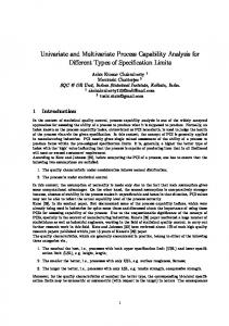
Cox Transform mation 5.2. Box-C The Box-C Cox transformation parameteer (λ) is estimated d by Minitab14 4 statistical sofftware and corresp ponding processs capability in ndices are determ mined. The acccuracy of the BoxCox transfformation is robust to depaartures from norm mal and it avo oids the troub ble of having to search for a suitable s metho od for each distrib bution encounttered in practicce.

416

c k . . .

C C C C

2.6080 3.9038 1.9032 1.9032

Thee Lambda tabble as shown in figure 5 con ntains an estimaate of lambda ((-0.21) which is the t value usedd in the transsformation. It also o includes the upper Confiddence Interval (0.4 46) and loweer Confidencee Interval (0.95 5),which are marked on thhe graph by verttical lines .In tthis case studyy, an optimal lam mbda value thhat correspondds to -0.21 is utiliized for trannsforming thhe data and calcculation of PC CIs. The figuree 6 shows the outp put of the Minnitab 14 statistiical software.

Y. Wooluru u,, D.R., Swam my, P. Nageshh

Box x-Cox Plot of Resistivity R Da ata Lower C L

175

Upper CL Lambda (using 95.0% confideence)

150

--0.21

Lower C L Upper C L

--0.95 0.46

Rounded Value

125 StDev

Estimate

0.00

100

75 Limit 50 -5.0

-2.5

0.0 0 Lamb bda

2.5

5.0

Figu ure 5. Box Cox x plot to estimaate optimal valuue of Process Cap pability of Res sistivity Data a Using Box-Cox Transformation Wiith Lambda = -0.221 U S L*

LS LL*

transformed datta

P rocess D ata LS L 100 Targ get * 500 USL mple M ean 241.35 S am S am mple N 100 S tD ev e (Within) 66.9729 S tD ev e (O v erall) 75.5519

Within O v erall P otential (Within) C apability Cp 0.988 C P L 1.099 C P U 0.877 C pk 0.877 C C pk 0.988

A fter Transformation LS L* * Targ get* U S L* mple M ean* S am S tD ev e (Within)* S tD ev e (O v erall)*

O v erall C apa bility

0.380189 * 0.271154 0.319472 0.0184948 0.0194258

Pp PPL PPU P pk C pm

0.28 O bse erv ed P erformance P P M < LS L 0.00 P P M > U S L 10000.00 P P M Total 10000.00

0.30 0

E xp. x Within P erformance P P M > LS L* 513.62 P P M < U S L* 4494.34 P P M Total 5007.96

0.32

0.34

0.36

0.944 1.044 0.833 0.833 *

0.3 38

E xp. O v erall P erform ance P P M > LS L* 887..14 P P M < U S L* 6436..14 P P M Total 7323..29

Figure 6. Prrocess capability Analysis usiing Box- Cox ttransformationn putation of PCIs P using Burr’s B 5.3. Comp method In this case study, theo oretical non-n normal distribution ns like expon nential, weibulll and

normal are ussed to model the response logn (ressistivity of ssilicon wafer)) .Individual disttribution identiification featurre in Minitab 14 is i used to com mpare the fit off distributions as shown s in the figgure 7.

417

Probabil ity Plot for Resistivity G ooodness of F it T est

E xponential - 95% C I 99.9

99

90

90

50 P er cent

P er cent

Lognorm al - 95 % C I 99.9

50 10

Loggnorm al A D = 0.435 P -V V alue = 0.295 ponential E xp A D = 23.551 P -V V alue < 0.003

10 1

1 0.1

100 1

200 R e s istiv itty

0.1 0.1

500

1 .0

1000.0

G aam m a A D = 0.793 P -V V alue = 0.042

G am m a - 95% C I

99.9

99.9

90

99

50

90

P er cent

P er cent

% CI Weibull - 95%

10.0 100.00 R e sistiv ity

10

Weeibull A D = 2.286 P -V V alue < 0.010

50 10

1 1

0.1 10

100 R e s istiv itty

1000

0.1

1 00

200 R e sistiv ity

500

Figurre 7. Probability y plots for the individual disttribution 5.3.1 Comparison C of altern native distributio ons with P-v values (For 95% Confidencce Interval) Individual distribution id dentification feature fe in statisticaal software (Minitab 14) is used to construct probability plots for said distribution ns in order to compare their

odness of fit w with the data. IIn this study, goo seveen distributionns are consideered to select the appropriate oone that fits thhe data. The logn normal distribbution providess the best fit in comparison c wiith other distribbutions as its p-vaalue (0.295) iss greater than critical value (0.0 05).

Table 5. Comparison of Alternative A Disstributions usin ng output from m probability pllot Distribution n type Weibull Exponential Log logistic Largest extreme value Lognormal Gamma Normal

AD A value 2.286 23.55 0.432 0.359 0.435 0.793 2.045

Process cap pability indicees for the case study data using lognormal disstribution are found M 14 statiistical through the output of Minitab software ass shown in the figure 8.

418

P-value < 0.010 < 0.003 0.242 > 0.250 0.295 0.042 < 0.005

6. Results and d Discussion n Thee following T Table 6 presennts the PCIs calcculation resultss of different m methods.

Y. Wooluru u,, D.R., Swam my, P. Nageshh

Table 6. Numerical N resullts for PCIs of Non-normal N an nd Classical M Method PCIs

Cp Cpl Cpu Cpk

Weeighted varriance method

Cleements Meethod

Obtained Results R Burr Box Cox Distriibution Tran nsformation

3.9 92 4.81 3.2 24 3.2 24

2.48 3.15 2.00 2.00

2.60 3.90 1.90 1.90

In this pap per, the Clemen nts, Burr, Weiighted variance, Box-Cox B transsformation meethods are revieweed and used to o estimate the PCIs for non-n normal quality characteristic data. PCIs of Classical method d are compared d with the PCIs of all the no on-normal meethods considered in the case study. In caase of classical method, m Cpu is over estimateed and Cpl is undeer estimated, when w compared d with PCIs of other non n-normal metthods. Weighted variance v (WV)) method givess good result but it requires manual m calculaations. Box- Cox x transformatiion method gives reasonably good resu ults compared d to classical method. m Burr peercentile metho od has been used effectively and a it shows better results com mpared to Clem ments method.

7. Concllusions In practicee, manufacturring processess that yields non n- normally distributed d datta are inevitable, therefore thee use of tradiitional process capability c ind dices to meeasure capability of o such processses give misleeading results. Box-Cox method is su uccessfully used to transform the non-normaal data to norrmally distributed data and estim mated the PCIs.. The obtain ned values off process capaability indices sh hows that thee capability of o the production process fo or controlling g the

0.98 1.09 0.87 0.87

Lognormal Model 0.97 1.01 0.93 0.93

Classical method m (Normality assumption) 22.37 22.50 22.19 22.19

resiistivity of siliccon wafer is iinadequate as all values v are lesss than 1.33 soo ,the process disp persion need to be reducedd and process meaan have to bbe shifted to ccloser to the targ get value of 2225 from existting mean of 241.79. Clements methodd is simple extension of the trad ditional 6σ m method, whichh takes into acco ount the posssible non-norm mality of the basiic data. Burrr-based methhod works well under disttributions thhat depart slightly or mod derately from normality (Skkewness ≤ 1.5)). Oveerall performannce of Box-Coox method is slig ghtly inferior than thee lognormal disttribution modeel, Lognormall distribution mod del exhibits thhat 6179 partss per million exceeding the sppecification lim mits but in casee of Box –C ox transformaation method 732 23 parts perr million exxceeding the speccification lim mits, hence it can be of data to modeling con ncluded that logn normal distribuution approachh is accurate onee. Thee estimates maade using the B Burr method, whiich are higheer than those made using Clements’s methhod are good indicator to help p quality conntrol engineeers be more atteentive to and foocus on processs adjustment and d improvement..

Referencces: Ahmed, S., Abdollanian, M., Zeephong gsekul, P. (200 08). Process cappability estimaation for nonnormal quality q characcteristics: A Comparison C off Clements, Buurr and Box-C Cox method. ANZIAM M Journal, 49(E EMAC 2007), C642-C665. C

419

Boyles, R.A. (1994). Process capability with asym mmetric toleraances. Commuunications in Statisticss: Simulation and a Communication, 23(3), 615-643 Castagliolaa, P. (1996). Evaluation off non-normal process capabbility indices using Burr’s distributiion. Quality En ngineering, 8, 587-593. 5 Chou, Y., Polansky, P A.M M., & Mason, R.L. R (1998). Trransforming noon-normal dataa to normality in statistiical process co ontrol. Journal of Quality Tecchnology, 30, 1133-141. Choi, I.S., & Bai, D.S. (1 1996). Process capability ind dices for skeweed populations .Proceedings of the 20 0 th Internation nal conference on computer an nd Industrial E Engineering, 12211-1214. Clements, J.A, (1989). Process P capabiility calculatio ons for non-noormal distributtions. Quality Progresss, 22, 95-100. Montgomeery, D. (1996). Introduction to Statistical Quality Q Controol. 5th edition.. Wiley, New York. Box, G.E.P P., & Cox, D.R. D (1964). An A analysis off transformatioons. Journal of the Royal Statistica al Society. Seriies B (Methodo ological), 26(2)), 211-252. Wu, H.H.,, Swain, J.J., Farrington, P.A., & Messim mer, L.S. (19999). A weighhted variance capabilitty index for General G non-no ormal processses. Quality annd Reliability Engineering Internatiional, 15, 397-402. Pearn, W.L L., Chen, K.S., & Lin G.H. (1995). A gen neralization of Clements metthod for nonnormal pearsonian p process with asym mmetric toleran nces. Internatiional journal of quality and Reliabiliity Managemen nt, 16(5), 507-5 521. Tang, L. & Than, S. (1999). Computting process capability indicces for non-noormal data: a review and comparrative study.. Qual. Relliab. Engng. Int., 15(55), 339-353. http://dx.doi.org/10.100 02/(sici)1099-1 1638(199909/1 10)15:53.00.co;2-a.

wamy Woolurru Yerrisw

Swa amy D.R.

Nagesh P.

JSS Acaademy of Techniical Educatio on, Bangalo ore India ysprabhu [email protected]

JSS Academy of Technical ucation, Edu Ban ngalore India drsw [email protected]

JSS Centre for M Management studies, Mysore India [email protected]

420

Y. Wooluru u,, D.R., Swam my, P. Nageshh