Process Mining Discovering Workflow Models from Event-Based Data A.J.M.M. Weijters
W.M.P van der Aalst
Eindhoven University of Technology, P.O. Box 513, NL-5600 MB, Eindhoven, The Netherlands, +31 40 2473857/2290 Abstract Contemporary workflow management systems are driven by explicit process models, i.e., a completely specified workflow design is required in order to enact a given workflow process. Creating a workflow design is a complicated time-consuming process and typically there are discrepancies between the actual workflow processes and the processes as perceived by the management. Therefore, we propose a technique for process mining. This technique uses workflow logs to discover the workflow process as it is actually being executed. The process mining technique proposed in this paper can deal with noise and can also be used to validate workflow processes by uncovering and measuring the discrepancies between prescriptive models and actual process executions.
1. Introduction During the last decade workflow management concepts and technology [2, 9, 10] have been applied in many enterprise information systems. Workflow management systems such as Staffware, IBM MQSeries, COSA, etc. offer generic modeling and enactment capabilities for structured business processes. By making graphical process definitions, i.e., models describing the life-cycle of a typical case (workflow instance) in isolation, one can configure these systems to support business processes. Besides pure workflow management systems many other software systems have adopted workflow technology. Despite its promise, many problems are encountered when applying workflow technology. As indicated by many authors, workflow management systems are inflexible and have problems dealing with change [2]. In this paper we take a different perspective with respect to the problems related to flexibility. We argue that many problems are resulting from a discrepancy between workflow design (i.e., the construction of predefined workflow models) and workflow enactment (the actual execution of workflows). Workflow designs are typically made by a small group of consultants, managers and specialists. As a result, the initial design of a workflow is often incomplete, subjective, and at a too high level. Therefore, we propose to “reverse the process”. Instead of starting with a workflow design, we start by gathering information about the workflow processes as they take place. We assume that it is possible to record events such that (i) each event refers to a task (i.e., a well-defined step in the workflow), (ii) each event refers to a case (i.e., a workflow instance), and (iii)
events are totally ordered. Any information system using transactional systems such as ERP, CRM, or workflow management systems will offer this information in some form. We use the term process mining for the method of distilling a structured process description from a set of real executions. The remainder of this paper is as follows. First we discuss related work and introduce some preliminaries including a modeling language for workflow processes and the definition of a workflow log. Then we present a new technique for process mining. Finally, we conclude the paper by summarizing the main results and pointing out future work.
2. Related Work and Preliminaries The idea of process mining is not new [3, 4, 5, 8]. However, most results are limited to sequential behavior. Cook and Wolf extend their work to concurrent processes in [5]. They also propose specific metrics (entropy, event type counts, periodicity, and causality) and use these metrics to discover models out of event streams. This approach is similar to the one presented in this paper. However, our metrics are quite different and our final goal is to find explicit representations for a broad range of process models, i.e., we generate a concrete Petri net rather than a set of dependency relations between events. Compared to existing work we focus on workflow processes with concurrent behavior, i.e., detecting concurrency is one of our prime concerns. Therefore, we want to distinguish AND/OR splits/joins explicitly. To reach this goal we combine techniques from machine learning with WorkFlow nets (WF-nets, [1]). WF-nets are a subset of Petri nets. Note that Petri nets provide a graphical but formal language designed for modeling concurrency. Moreover, the correspondence between commercial workflow management systems and WF-nets is well understood [1, 2, 7, 9, 10].
T12 T9 Sb
T1
P1 T2
P2
T3
P4
T5
P6
P9
T11
p10
T13
Se
T8
P3
T4
P5
T6
P7
T10
P8
T7
Figure 1: example of a workflow process modeled as a Petri net. Workflows are by definition case-based, i.e., every piece of work is executed for a specific case. Examples of cases are a mortgage, an insurance claim, a tax declaration, an order, or a request for information. The goal of workflow management is to handle cases as efficient and effective as possible. A workflow process is designed to handle similar cases. Cases are handled by executing tasks in a specific order. The workflow process model specifies which tasks need to be executed and in what order. Petri nets [6] constitute a good starting point for a solid theoretical foundation of workflow
management. Clearly, a Petri net can be used to specify the routing of cases (workflow instances). Tasks are modeled by transitions and causal dependencies are modeled by places and arcs. As a working example we use the Petri net shown in Figure 1. The transitions T1, T2, …, T13 represent tasks, The places Sb, P1, …, P10, Se represent the causal dependencies. In fact, a place corresponds to a condition that can be used as pre- and/or post-condition for tasks. An AND-split corresponds to a transition with two or more output places (from T2 to P2 and P3), and an AND-join corresponds to a transition with two or more input places (from P8 and P9 to T11). OR-splits/ORjoins correspond to places with multiple outgoing/ingoing arcs (from P5 to T6 and T7, and from T7 and T10 to P8). At any time a place contains zero or more tokens, drawn as black dots. Transitions are the active components in a Petri net: they change the state of the net according to the following firing rule: (1) A transition t is said to be enabled iff each input place of t contains at least one token. (2) An enabled transition may fire. If transition t fires, then t consumes one token from each input place p of t and produces one token for each output place p of t. A Petri net which models the control-flow dimension of a workflow, is called a WorkFlow net (WF-net) [1]. A WF-net has one source place (Sb) and one sink place (Se) because any case (workflow instance) handled by the procedure represented by the WFnet is created when it enters the workflow management system and is deleted once it is completely handled, i.e., the WF-net specifies the life-cycle of a case. An additional requirement is that there should be no “dangling tasks and/or conditions”, i.e., tasks and conditions which do not contribute to the processing of cases. Therefore, all the nodes of the workflow should be on some path from source to sink. Although WF-nets are very simple, their expressive power is impressive. In this paper we restrict our self to so-called sound WF-nets [1]. A workflow net is sound if the following requirements are satisfied: (i) termination is guaranteed, (ii) upon termination, no dangling references (tokens) are left behind, and (iii) there are no dead tasks, i.e., it should be possible to execute an arbitrary task by following the appropriate route. Soundness is the minimal property any workflow net should satisfy. In this paper, we use workflow logs to discover workflow models expressed in terms of WF-nets. A workflow log is a sequence of events. For reasons of simplicity we assume that there is just one workflow process. Note that this is not a limitation since the case identifiers can be used to split the workflow log into separate workflow logs for each process. Therefore, we can consider a workflow log as a set of event sequences where each event sequence is simply a sequence of task identifiers. Formally, WL⊆T* where WL is a workflow log and T is the set of tasks. An example event sequence of the Petri net of Figure 1 is given below: T1, T2, T4, T3, T5, T9, T6, T3, T5, T10, T8, T11, T12, T2, T4, T7, T3, T5, T8, T11 ,T13
Using the definitions for WF-nets and event logs we can easily describe the problem addressed in this paper: Given a workflow log WL we want to discover a WF-net that (i) potentially generates all event sequence appearing in WL, (ii) generates as few event sequences of T*\WL as possible, (iii) captures concurrent behavior, and (iv) is as simple and compact as possible. Moreover, to make our technique practical applicable we want to be able to deal with noise.
3. Process mining technique In this section we present the details of our process mining technique. We can distinguish three mining steps: Step (i) the construction of a dependency/frequency table (D/F-table), Step (ii) the induction of a D/F-graph out of a D/F-table, and Step (iii) the reconstruction of the WF-net out of the D/F-table and the D/F graph.
3.1 Construction of the dependency/frequency table The starting point of our workflow mining technique is the construction of a D/F-table. For each task A the following information is abstracted out of the workflow log: (i) the overall frequency of task A (notation #A), (ii) the frequency of task A directly preceded by another task B (notation BB), (iv) the frequency of A directly or indirectly preceded by another task B but before the next appearance of A (notation BB), and finally (vi) a metric that indicates the strength of the causal relation between task A and another task B (notation AàB). T10 T5 T11 T13 T9 T8 T3 T6 T7 T12 T1 T2 T4
#B 1035 3949 1994 1000 1955 1994 3949 1035 959 994 1000 1994 1994
B
B 581 168 0 0 46 31 209 0 0 0 0 0 0
BB 1035 897 1035 687 538 925 808 348 241 505 0 505 505
Aà àB 0.803 0.267 0.193 0.162 0.161 0.119 0.019 0.000 -0.011 -0.093 -0.246 -0.487 -0.825
Table 1: an example D/F-table for task T6. Metric (i) through (v) seems clear without extra explanation. The underlying intuition of metric (vi) is as follows. If it always the case that, when task A occurs, shortly later task B also occurs, than it is plausible that task A causes the occurrence of task B. On the other hand, if task B occurs (shortly) before task A it is implausible that task A is the cause of task B. Bellow we define the formalization of this intuition. If, in an event stream, task A occurs before task B and n is the number of intermediary events between them, the AàB-causality counter is incremented with a factor (δ)n. δ is a causality fall factor (δ in [0.0…1.0]). In our experiments δ is set to 0.8. The effect is that the contribution to the causality metric is maximal 1 (if task B appears directly after task A then n=0) and decreases if the distance increases. The process of looking forward from task A to the occurrence of task B stops after the first occurrence of task A or task B. If task B occurs before task A and n is again the number of intermediary events between
them, the AàB-causality counter is decreased with a factor (δ)n. After processing the whole workflow log the AàB-causality counter is divided by the overall frequency of task A (#A). Given the process model of Figure 1 a random workflow log with 1000 event sequences (23573 event tokens) is generated. As an example Table 1 shows the abovedefined metrics for task T6. Notice that the task T6 belongs to one of two concurrent event streams (the AND-split in T2). It can be seen from Table 1 that (i) only the frequency of T6 and T10 are equal (#T6=#T10=1035), (ii) T6 is never directly preceded by T10 (BB=581), (iv) T6 is sometimes preceded by T10 (BB = #T6=1035). Finally, (vi) there is strong causality relation from T6 to T10 (0.803) and to a certain extent to T5 (0.267). However, T6 is from time to time directly preceded by T5 (BB ≥ σ) AND (BB ≥ σ) contains a threshold value σ. If we know that we have a workflow log that is totally noise free, then every task-patron-occurrence is informative. However, to protect our induction process against inferences based on noise, only task-patron-occurrences above a threshold frequency σ are reliable enough for our induction process. To limit the number of parameters the value σ is automatically calculated using the following equation: σ =1+Round (N*#L/#T). N is the noise factor, #L is the number of trace lines in the workflow log, and #T is the number of elements (different tasks) in the node set T. In our working example σ =1+ Round(0.05*1000/13)=5. It is clear now that the second condition demands that the frequency of A>B is equal or higher than the threshold value σ. Finally, the third condition states the requirement that the frequency of BT9 and T9>>T9 and T9T9 and T9>>B ≥ 0.4 * #A) AND (BB) THEN ∈ T To prevent our heuristic from breaking done in the case of some noise, we use an about symbol (≈) instead of the equality symbol (=). Again, the noise factor N is used to specify what we mean with ‘about equal’: x ≈ y iff the relative difference between them is less than N.
3.3 Generating WF-nets from D/F-graphs Given a workflow log it appears relatively simple to find the corresponding D/F-graph. But, the types of the splits and joins are not yet represented in the D/F-graph. However information in the D/F-table contains useful information to indicate the type of a join or a split. For instance, if we have to detect the type of a split from A to B AND/OR C, we can look in the D/F-table to the values of CC. If A is an AND-split we expect a positive value for both CC (because the pattern B, C and the pattern C, B can appear). If it is a OR-split the patterns B,C and C,B will not appear. The pseudo code for an algorithm based on this heuristic is given in Table 2. Suppose, task A is directly preceded by the task B1 to Bn. Set1 to Setn are empty sets. After applying the algorithm all OR-related tasks are collected in a set Seti. All not empty sets are in the AND-relation. We can apply an analogue algorithm to reconstruct the type of a join. For instance, applying the algorithm on the T11-join will result in two sets {T7, T10} and {T8} or in proposition-format ((T7 OR T10) AND T8). Using this algorithm we were able to reconstruct the types of the splits and joins appearing in our working example and to reconstruct the complete underlying WF-net. In the next section we will report our
experimental results of applying the above-defined heuristics on other workflow logs, with and without noise. For i:=1 to n do For j:=1 to n do OK:=False; Repeat If ∀ X∈ Setj [(Bi>X < σ) AND (X>Bi < σ )] then Begin Setj := Setj ∪ {Bi }; OK:=True End; Until OK; End j do; End i do; Table 2: the pseudo code used to reconstruct the types of the splits and joins of a D/F-graph.
3.4 Experiments To test our approach we use the Petri-net-representations of six different workflow models. The complexity of these models range from comparable with the complexity of our working model of Figure 1 (13 tasks) to models with 16 tasks. All models contain concurrent processes and loops. For each model we generated three random workflow logs with 1000 event sequences: (i) a workflow log without noise, (ii) one with 5% noise, and (iii) a log with 10% noise. Below we explain what we mean with noise. To incorporate noise in our workflow logs we define four different types of noise generating operations: (i) delete the head of a event sequence, (ii) delete the tail of a sequence, (iii) delete a part of the body, and finally (iv) interchange two random chosen events. During the deletion-operations minimal one event, and maximal one third of the sequence is deleted. The first step in generating a workflow log with 5% noise is a normal random generated workflow log. The next step is the random selection of 5% of the original event sequences and applying one of the four above described noise generating operations on it. Due to lack of space it is not possible to describe all workflow models and the resulting D/F-graphs in detail. However, applying the above method on the six noise free workflow logs results in six perfect D/F-graphs (i.e. all the connections are correct and there are no missing connections), and exact copies of the underlying WF-nets. If we add 5% noise to the workflow logs, the resulting D/F-graphs and WF-nets are still perfect. However, if we add 10% noise to the workflow logs one D/F-graph is still perfect, five D/F-graphs contains one error. All errors are caused by the low threshold value σ=5 in rule (1), resulting in an unjustified applications of this rule. If we increase the noise factor value to a higher value (N=0.10), the automatically calculated threshold value σ increases to 9 and all five errors disappear and no new errors occur.
4. Conclusion In this paper we introduced the context of workflow processes and process mining, some preliminaries including a modeling language for workflow processes, and a definition of
a workflow log. Hereafter, we presented the details of the three steps of our process mining technique: Step (i) the construction of the D/F-table, step (ii) the induction of a D/F-graph out of a D/F-table, and step (iii) the reconstruction of the WF-net out of the D/F-table and the D/F graph. In the experimental section we applied our technique on six different sound workflow models with about 15 tasks. All models contain concurrent processes and loops. For each workflow model we generated three random workflow logs with 1000 event sequences: (i) without noise, (ii) with 5% noise, and (iii) with 10% noise. Using the proposed technique we were able to reconstruct the correct D/F-graphs and WF-nets. The experimental results with the workflow logs with noise indicate that our technique seems robust in case of noise. Notwithstanding the reported results there is a lot of future work to do. First, the reported results are based on a limited number of experimental results; more experimental work must be done. Secondly, we will try to improve the quality and the theoretical basis of our heuristics. Can we for instance prove that our heuristic is successful applicable to logs from for instance free-choice WF-nets? Finally, we will extend our mining technique in order to enlarge the set of underlying WF-nets that can be successfully mined.
References [1] W.M.P. van der Aalst. The Application of Petri Nets to Workflow Management. The Journal of Circuits, Systems and Computers, 8 (1):21-66, 1998. [2] W.M.P. van der Aalst, J. Desel, and A. Oberweis, editors. Business Process Management: Models, Techniques, and Empirical Studies, volume 1806 of Lecture Notes in Computer Science. Springer-Verlag, Berlin, 2000. [3] R. Agrawal, D. Gunopulos, and F. Leymann. Mining process models from workflow logs. In the proceedings of the Sixth International Conference on Extending Database Technology, pages 469-483, 1998. [4] J.E. Cook and A.L. Wolf. Discovering Models of Software Processes from Event-Based Data, ACM Transactions on Software Engineering and Methodology, 7(3):215-249, 1998. [5] J.E. Cook and A.L. Wolf. Event-Based Detection of Concurrency. In Proceedings of the Sixth International Symposium on the Foundations of Software Engineering (FSE-6), Orlando, FL, November 1998, pp. 35-45. [6] J. Desel and J. Esparza. Free Choice Petri Nets, volume 40 of Cambridge Tracts in Theoretical Computer Science. Cambridge University Press, Cambridge, UK, 1995. [7] C.A. Ellis and G.J. Nutt. Modelling and Enactment of Workflow Systems. In M. Ajmone Marsan, editor, Application and Theory of Petri Nets 1993, volume 691 of Lecture Notes in Computer Science, pages 1-16. Springer, Berlin, Germany, 1993. [8] J. Herbst. A Machine Learning Approach to Workflow Management. In 11th European Conference on Machine Learning, volume 1810 of Lecture Notes in Computer Science, pages 183-194, Springer, Berlin, Germany, 2000. [9] S. Jablonski and C. Bussler. Workflow Management: Modeling Concepts, Architecture, and Implementation. International Thomson Computer Press, 1996. [10] P. Lawrence (editor). Workflow Handbook 1997, Workflow Management Coalition. John Wiley and Sons, New York, 1997.