Discovering Compressing Serial Episodes from Event Sequences

arXiv:1401.1043v2 [cs.DB] 11 Oct 2014

Under consideration for publication in Knowledge and Information Systems

Discovering Compressing Serial Episodes from Event Sequences Ibrahim A1 , Shivakumar Sastry2 , P.S. Sastry1 1 Department 2 Department

of Electrical Engineering, Indian Insitute of Science, Bangalore of Electrical and Computer Engineering Unversity of Akron

Abstract. Most pattern mining methods yield a large number of frequent patterns and isolating a small, relevant subset of patterns is a challenging problem of current interest. In this paper we address this problem in the context of discovering frequent episodes from symbolic time series data. Motivated by the Minimum Description Length principle, we formulate the problem of selecting relevant subset of patterns as one of searching for a subset of patterns that achieves best data compression. We present algorithms for discovering small sets of relevant non-redundant episodes that achieve good data compression. The algorithms employ a novel encoding scheme and use serial episodes with inter-event constraints as the patterns. We present extensive simulation studies with both synthetic and real data, comparing our method with the existing schemes such as GoKrimp and SQS. We also demonstrate the effectiveness of these algorithms on event sequences from a composable conveyor system; this system represents a new application area where use of frequent patterns for compressing the event sequence is likely to be important for decision-support and control. Keywords: Frequent Episodes, Serial Episodes, Mining Event Sequences, Discovering Compressing Patterns, MDL, Inter-Event-Time constraints.

1. Introduction Frequent pattern mining is an important problem in the area of data mining that has diverse applications in a variety of domains [11]. Even though many algorithms have been proposed for frequent pattern mining, most of these methods produce a large number of frequent patterns. In addition, the patterns found are often redundant in the sense that many patterns are very similar. The redundancy and the large volume of the patterns discovered makes it difficult to use the mined patterns to gain useful insights into the data or to use them to extract rules which are effective for prediction, classification etc., in the application domain. Thus, finding a small set of non-redundant, relevant and informative pat-

2

Ibrahim. A et al

terns that succinctly characterize the data, is an important problem of current interest. There are many methods that are proposed for reducing the number of extracted frequent patterns. Many such methods concentrate on eliminating patterns that are deemed to be non-informative given the other frequent patterns. For example, in the context of transaction datasets, concepts such as closed [19, 26], non-derivable [5] and maximal [4, 15] itemsets were suggested to reduce the number of frequent itemsets extracted. Similarly, closed sequential patterns were proposed for sequence datasets [6, 25, 30]. Even though such methods result in some reduction in the number of patterns returned by the algorithm, the number of patterns still remains substantial. Also, the redundancy in the final set of patterns is, often, still large. Recently, there have been other efforts for finding a small set of informative patterns that best describes the data. For example, [7] proposes a method for summarization of transaction datasets based on some ideas from information theory. They propose a method of selecting a subset of frequent itemsets to achieve a good lossy summarization of the database. Here each transaction is summarized by one itemset with as little loss of information as possible. In [27], which also proposes a lossy summarization, each transaction is covered, partially, by the largest frequent itemset. In contrast to these methods, [22, 24] propose lossless summarization of transaction datasets using the Minimum Description Length (MDL) principle. A related approach called Tiling was used by [9, 29], again for a lossless summarization of the data. In this paper, we address the problem of discovering a set of patterns that can achieve succinct lossless representation of temporal sequence data. We present algorithms that discover a small set of relevant patterns (which are special forms of serial episodes) which summarize the data well. We use the MDL principle [10] to define what we mean by summarizing the data well. The basic idea is that a set of patterns characterizes or summarizes the data sequence well, if the set of patterns can be used as a model to encode the data to achieve good compression. As mentioned above, the MDL principle has been used earlier to obtain relevant and non-redundant subsets of frequent patterns. The idea was first explored by the Krimp algorithm [24] in the context of transaction data. This algorithm selects a subset of frequent itemsets which, when used for encoding the database, achieves good compression. Each selected itemset is assigned a code with shorter code lengths assigned to higher frequency itemsets. The algorithm tries to encode each transaction with the codes of itemsets which have minimal code lengths and which cover maximum number of items. Similar strategies have been proposed for sequence data also [12, 13, 23]. For sequential data, unlike in the case of transaction data, the temporal ordering is important and this presents additional complications while encoding the data. For example, consider a single transaction, t = ABCD from a transaction database and two itemsets AC and BD. The codewords for AC and BD can encode the transaction t (since the transaction is just a set of items). Now consider a sequence s = ABCD and two serial episodes A → C and B → D. Even though the occurrences of A → C and B → D would cover the sequence s, this information alone is insufficient for encoding the sequence. Since the order of events is important in sequential data, in order to get back the exact sequence, one needs to specify where exactly the occurrences of the episodes happen in the sequence. For example, we need to know that the A and C in the occurrence of A → C are not contiguous and that there is a B in the gap between them. One

Discovering Compressing Serial Episodes from Event Sequences

3

needs to have some way of taking care of such gaps while encoding the data with the occurrences of some frequent episodes. In general, the events in a sequence constituting an episode occurrence need not be contiguous, and different occurrences can have arbitrary temporal overlaps. An encoding scheme should be able to properly take care of this. The previous approaches for using the MDL principle to summarize sequence data [12,13,23], explicitly record such gaps while encoding data, thus significantly increasing the encoding length. While the methods presented in [13, 23] consider only sequential data without time stamps, the method in [12] does encode event sequences with time stamps also; but the encoding scheme needs to individually encode each event time stamp. In some cases, the resulting encoding may become even longer than the raw data [12]. For the problem of identifying a relevant subset of frequent patterns, we are using the encoded length (of the data encoded with a subset of patterns), only as a figure of merit to compare different subsets. Hence, the fact of the encoding length becoming more than the raw data is, per se, not disallowed. However, the underlying philosophy of MDL principle suggests that one needs a good level of data compression to have confidence in a model. For example, even if the sequence data is iid noise and has no temporal structure, there would be some subset of patterns that would achieve lower encoded data length than other subsets. However, one expects that even the best such subset here would not achieve any appreciable level of data compression, thus suggesting that there are no significant temporal regularities in the data. On the other hand, for a sequence with significant temporal regularities, one expects good compression of the data sequence, if the method is able to discover the best temporal patterns and encode the sequence with them. In general, if we can discover some long episodes which occur many times, then their occurrences can encode many events in the data sequence thus giving rise to the possibility of data compression. In this paper, we consider summarizing event sequences (having time stamps on events) using a pattern class consisting of serial episodes with fixed interevent times. We present algorithms for discovering a small subset of relevant frequent episodes that result in good compression of the data sequence. The novelty of our approach is that, in contrast to the existing schemes in [12,13,23], our method does not need to explicitly encode gaps in episode occurrences and the encoding scheme is such that we can retrieve the full data sequence with the time stamps on events, from the encoded sequence. The encoding of the data consists of only the start times of occurrences of various episodes; the gaps are determined from the fixed inter-event time constraints of the episodes. We show through simulations that our method results in better data compression. We also show, through empirical experiments, that the episodes that result in good data compression are also highly relevant for the dataset. We also illustrate the benefits of our algorithm using an application, where it is important to both find relevant patterns and achieve good data compression. We consider streams of sensor-data from a composable conveyor system (CCS) [3, 21] that is useful for materials handling. In this system, several conveying units are dynamically composed to achieve the application objectives; consequently, utilizing the data streams to diagnose or reconfigure the system is important. The data consists of a sequence of predefined events such as, package entered a unit, package exited a unit, package arrived at an input port, etc. Such events occur at various units in the conveyor system during its routine operation. On this data stream, frequent serial episodes represent the routes (sequence of

4

Ibrahim. A et al

units) over which packages were transported in the conveyor system. The interevent times corresponds to the various physical constraints such as time required for a package to move through a specific unit, the time required for two adjacent units to complete a handshake protocol to transfer packages between them etc. Thus a small set of relevant episodes can provide a good summary of the events in the conveyor system. We can use the discovered set of relevant episodes to achieve a lossless compression of the original temporal event sequence to support remote monitoring, diagnostics and visualization activities. We explain the system in more detail in Section 5.1.1. Using data obtained from a high-fidelity discrete event simulator of such conveyor systems, we demonstrate that our algorithms: (a) unearth a small set of relevant episodes that capture the essence of the transport through the system, and (b) our scheme achieves good data compression. Even though our method is motivated by the above application, we show that our method is effective with other general sequential data as well. Apart from conveyor system data streams, we show the effectiveness of our methods with text data as well as on a few other real data sequences. These are the data sets that are used to illustrate the effectiveness of the algorithms presented in [12,13,23]. We compare the performance of our algorithm with these methods on these data sets as well as on the composable conveyor system data. The rest of the paper is organized as follows. In Section 2, we briefly review the formalism of episodes, introduce the new subclass of serial episodes and formally state the problem. Section 3 describes our encoding scheme for temporal data using our episodes. The various algorithms for mining and subset selection are explained in Section 4 and the experimental results are given in Section 5. We conclude the paper in Section 6.

2. Problem Statement 2.1. Fixed Interval Serial Episodes The data we consider is a sequence of n events denoted as D = h(E1 , t1 ), (E2 , t2 ), . . . , (En , tn )i, where ti ≤ ti+1 , and if ti = ti+1 , then Ei 6= Ei+1 , where Ei ∈ Σ, is the event-type, Σ is the alphabet and ti ∈ Z+ is the time stamp of the ith event. Note that we can have multiple events (of different types) all occurring at the same time instant. A k-node serial episode α is denoted as e1 → e2 → · · · → ek where ei ∈ Σ, ∀i. An occurrence of α in D is a mapping h : {1 . . . k} → {1 . . . n}, such that ei = Eh(i) , 1 ≤ i ≤ k and th(i) < th(j) , for i < j. An occurrence can be denoted by (th(1) , . . . , th(k) ), the event times of the events constituting the occurrence. We call the interval [th(1) , th(k) ] as the occurrence window of this occurrence. (If k = 1, then for the 1-node episode, the occurrence window is essentially a number which is the event time of that event). Consider an example event sequence D1 = h(A, 1), (A, 2), (B, 3), (E, 4), (A, 5), (B, 6), (C, 6), (B, 7), (D, 8), (C, 10), (E, 11)i (1) In the data sequence given in (1), a few occurrences of episode A → B → C are (1, 3, 6), (2, 3, 6), (5, 6, 10). A fixed interval serial episode is a serial episode with fixed inter-event gaps.

Discovering Compressing Serial Episodes from Event Sequences ∆

5 ∆

∆k−1

2 1 · · · −−−→ ek . We e2 −−→ A fixed interval serial episode is denoted as β = e1 −−→ will be considering the class of fixed interval serial episodes, where ∆i ≤ Tg , ∀i, with Tg being a user specified upper bound on allowable gap. An occurrence of β in D is a mapping h : {1 . . . k} → {1 . . . n}, such that ei = Eh(i) , 1 ≤ i ≤ k and th(i+1) − th(i) = ∆i > 0, for 1 ≤ i < k. For example, in sequence D1 in (1), there

2

3

are two occurrences of episode A − →B− → C, namely (1, 3, 6) and (5, 7, 10). Note that the time of the first event of an occurrence completely specifies the entire occurrence. This property of the fixed interval serial episodes allows us to design a coding scheme that results in data compression. A k-node fixed interval serial ∆

∆

∆k−1

2 1 · · · −−−→ ek is called injective if ei 6= ej , ∀i, j, i 6= j. e2 −−→ episode α = e1 −−→ In the literature, different notions of frequency are defined for episodes depending on the type of occurrences we count. (For a discussion on various frequencies see [2]). An episode is said to be frequent if its frequency is above a given threshold. In this paper, we consider the number of distinct occurrences as the frequency. Two occurrences are distinct if none of the events of one occurrence is among events of the other. More formally, a set of occurrences, {h1 , h2 , . . . , hm } of an episode α are distinct if for any k 6= k 0 , hk (i) 6= hk0 (j), ∀i, j. This is a natural notion of frequency for an injective fixed interval serial episode because any pair of its occurrences with different start times will always be distinct. In this paper, we consider injective fixed interval serial episodes and from now on we refer to injective fixed interval serial episodes simply as episodes whenever there is no scope for confusion.

2.2. Selecting a Subset of Episodes Using the MDL Principle Pattern mining algorithms often output a large number of frequent episodes. Our goal is to isolate a small subset of them which are non-redundant and are relevant for the data. To formalize this goal, we use the MDL principle which views learning as data compression. The idea is that if we can discover all the relevant regularities in the data, then an encoding based on these would result in data compression [10]. Thus, the goal is to find a model which allows us to encode the data in a compact fashion. Given any model, H, let L(H) denote the length for encoding the model H and let L(D|H) be the length of the data when encoded using the model H. Given an encoding scheme, under the MDL principle our goal is to find a model H that minimizes total encoded length, L(H, D) = L(H) + L(D|H). For us, different models correspond to different subsets of the set of frequent fixed interval serial episodes. As mentioned earlier, an occurrence of such an episode is uniquely specified by its start time. Hence, by giving the code for the identity of the episodes and a list of start times, we can code all the events constituting the occurrences of this episode. (We explain our encoding scheme in the next section). Thus, large episodes with many occurrences would account for a large number of events in the data sequence thus decreasing L(D|H). Another advantage of our use of the MDL principle is that it inherently takes care of redundancy. Selecting episodes with minimal overlap among their occurrences would help reduce the final encoded length. Under MDL, we are looking at lossless coding and hence the occurrences of the selected subset of episodes have to cover the entire dataset; i.e., every event in the data sequence should be part of an occurrence of (at least) one of

6

Ibrahim. A et al

Table 1. A data sequence and its encoding D2 = h(D, 1)(A, 2)(C, 3)(E, 3)(A, 4)(B, 4)(C, 5)(D, 5) (B, 6)(C, 7)(E, 7)(C, 8)(C, 9)i Size of Episode

Episode Name

3

A− →B− →C

3 1

2

1

2

2

D− →E− →C C

No. of Occurrences

List of Occurrences

2

h2, 4i

2 2

h1, 5i h3, 8i

the selected set of episodes. We can always ensure this by adding a few 1-node episodes, as needed. We will give details of our encoding in the next section. Our main problem can now be stated as below Problem 1. Given a data sequence D and a set of (frequent) fixed interval serial episodes, C = {C1 , C2 , . . . , CN }, find the subset H ∗ ⊆ C such that H ∗ = arg min{L(H) + L(D|H)} H⊆C

3. The Encoding Scheme for Data In this section, we explain our encoding scheme and derive the expression for encoded data length.

3.1. Encoding Each model H is a set of some fixed interval serial episodes whose occurrences cover the data. Given such an H, which forms the dictionary, the data is then encoded by specifying the start times of selected occurrences of the episodes. We explain our encoding scheme through an example. Table 1 shows a data sequence D2 and its encoding using three arbitrarily selected episodes. Each row in the table describes one of the episodes used and the encoding for the part of the data, covered by the occurrences of that episode. There are four columns in the table. Column 1 gives the size of the episode in that row and the second column specifies the episode. The third column gives the number of occurrences of that episode (used for encoding) and the last column gives a list of start times. Hence 2 1 the first row of Table 1 specifies: a 3-node episode, namely, A − →B− → C and two of its occurrences starting at times 2 and 4. Thus, the first row of Table 1 accounts for the events (A, 2), (B, 4), (C, 5) and (A, 4), (B, 6), (C, 7) in the data, which are 2 1 the events constituting the two occurrences of the episode A − →B− → C starting at time stamps 2 and 4 respectively. We can think of the first two columns of the table as our dictionary and the last two columns of the table as the encoding of the data. Note that the seventh event in D2 , (C, 5), is part of the occurrence 2 1 2 2 of A − →B − → C starting at 2 and of D − →E − → C starting at 1. While this is allowed in our encoding, minimizing such overlaps would improve total encoded length. In fact, we use injective fixed interval serial episodes in order to avoid overlap of different occurrences of the same episode, since, as we mentioned earlier, occurrences of injective fixed interval serial episodes starting at different

Discovering Compressing Serial Episodes from Event Sequences

7

time stamps are distinct. occurrences In Table 1, the first two episodes account for all but two events in the data and hence we added a 1-node episode (in row 3 of the table) to ensure that we cover the full data sequence. Our final encoded sequence would be a table like this. Each entry in the table is essentially a series of integers and our final encoded data would consists of a series of integers obtained by stringing together the rows in order.

3.2. Decoding In this section we discuss how to decode the encoded data. The encoded data consists of rows of a table, with each row specifying an episode and its occurrences. In each row, we read the first value, which is the size of the pattern. If this value is k, the next 2k −1 integers correspond to the codes of the event types (k units) followed by the inter event gaps (k − 1 units). The next value in the encoded sequence corresponds to the number of occurrences of the episode. We then need to read that many values to obtain all the occurrence start times of that episode and complete reading the current row. Since we know when the row is complete, the next integer would be the first entry of the next row and we repeat the same process as above. From each start time of occurrence of an episode, we can roll out the corresponding events because we know the event types and the inter-event gaps. Once we are done with rolling out all the occurrences of all the episodes, we have to just sort the events based on the time stamps and delete duplicate occurrences1 to retrieve back the original data sequence.

3.3. Length of the Encoding We have seen that once the dictionary is fixed, the data encoding is just a series of integers denoting the start times of occurrences of the patterns in the dictionary. Even though, we could use bit level integer encoding schemes like Elias codes [13, 28] and Universal codes [20, 23] for encoding integers (and have the size of encoding dependent on the value of the integer), we use the notion of fixed memory units instead. The reason being that, the MDL principle looks at utilizing the regularity in data to compress the data and hence the level of compression should not depend on the magnitude of data item. For example, the value of a time stamp, per se, does not have any regularity and the compression achieved by the encoding scheme, hence, should not be dependent on the values of time stamps. Therefore, for calculating the total encoded lengths we consider event types and times to be integers and assume that each such integer accounts for one unit in the encoded length. Since our aim is to compare different models, keeping all lengths in terms of one unit per integer is sufficient for us. (Here we are assuming that, in describing episodes in the dictionary, all event-types take the same amount of memory. We could, of course, use codes such as Hamming codes, to reduce expected length of representation of episodes. We do not consider such extra compression here). Later on, while comparing our method with the various

1

Note that while events of different types can occur with the same time stamp, events with same event-type cannot co-occur at the same time instant; hence we can easily spot duplicates while decoding.

8

Ibrahim. A et al

other methods, we use bit level encoding for calculating lengths of integers so that we can easily compare with the results of other algorithms. Let model H contain the episodes {F1 , F2 , . . . , FK }, with |Fi | denoting the size of episode Fi . Each episode needs one integer to represent its size, |Fi | integers for representing the event types and (|Fi | − 1) integers for inter-event PK gaps. Hence the first two columns of the table need i=1 (1 + |Fi | + |Fi | − 1) = PK i=1 2|Fi | integers. This is L(H). Let fi be the number of occurrences of Fi listed in the column 4 of our table. PK Then, columns 3 and 4 together need i=1 (fi + 1) integers. This is L(D|H). Thus for the model H, the total encoded length is L(H, D) = L(H) + L(D|H) =

K X i=1

2|Fi | +

K X (fi + 1)

(2)

i=1

For the encoding given by Table 1, the length for the first row is 1+(3+2)+1+2 = 9 and it is easy to see that the total encoded length is 9 + 9 + 5 = 23. The length of raw data can be taken to be 2|D| where |D| is the number of events in the data. However, taking this as the length of uncompressed data may result in higher value for the compression achieved by an algorithm. This is because, even without finding any patterns, we can represent the raw data more compactly by simply using only 1-node episodes in our encoding. If we have M event types then we use M 1-node episodes for encoding. The total encoded length, using Equation (2), and taking K = M would be 2M + |D| + M . PM (Note that i=i fi = |D|, because all occurrences of the M 1-node episodes, together would exactly cover the data; also no event in the data would be part of occurrences of two different 1-node episodes). We call such an encoding trivial encoding. For the data sequence D2 , the length for trivial encoding would be 5 × 2 + 13 + 5 = 28. Even though in this example the length of the trivial encoding is more than 2|D|, for real datasets we would have |D|  M and hence total encoded length of trivial encoding would be less than 2|D|. Hence in calculating data compression with our method, we compare the length of the trivial encoding with the length of the encoding using selected episodes.

4. Algorithms In this section, we consider algorithms for discovering a subset of episodes which achieves good compression. Finding the optimal subset of episodes to minimize total encoded length is known to be NP-Hard [12, 23]. Hence the methods we present here are approximation algorithms to Problem 1. We begin by presenting algorithm CSC-1 (CSC is for Constrained Serial episode Coding), which is a two phase method. This consists of discovering all frequent episodes through a depth-first search algorithm followed by a greedy method of selecting a subset based on maximum coverage and minimum overlap. We then present algorithm CSC-2, which directly mines for relevant fixed interval serial episodes from the data without first discovering all frequent episodes.

Discovering Compressing Serial Episodes from Event Sequences

9

Algorithm 1 MineEpisodes(D, Tg , fth ) Input: Sequence data D, the maximum inter-event gap Tg and frequency threshold, fth Output: The set of frequent episodes, C 1: A ← Set of all frequent 1-node episodes in D, along with occurrence lists. 2: for all A ∈ A do 3: ExploreDFS(A, A, Tg , fth ) . All the frequent episodes . are added to the global list C 4: end for Algorithm 2 ExploreDFS(α, A,Tg , fth ) Input: Episode α with its occurrence list; A: the set of frequent one node episodes with its occurrence lists; Tg : Maximum inter-event gap; fth : frequency threshold Output: The set of frequent episodes C. 1: for all A ∈ A\{set of event-types in α} do 2: occurrlist-for-delta ← find-lists(α, A, Tg ) 3: for j = 1 → Tg do 4: if |occurrlist-for-delta(j)| ≥ fth × |D| then 5: 6: 7: 8: 9: 10: 11:

j

β ← (α − → A) β.occurrencelist ← occurrlist-for-delta(j) C ←C∪β ExploreDFS(β, A, Tg ) end if end for end for

4.1. First Algorithm: CSC-1 We first explain our depth-first mining algorithm and the basis for the greedy strategy for subset selection before describing the full CSC-1 algorithm (which is listed as Algorithm 4).

4.1.1. Mining To obtain all frequent injective fixed interval serial episodes, we use a depth-first (also known as pattern-growth) strategy using occurrence windows. See [1, 17] for more details on depth-first strategies using occurrence windows. The basic idea is as follows. First we find all 1-node frequent episodes (which are eventtypes that occur often enough) and for each frequent 1-node episode, keep its occurrence list which is a list of event times where the 1-node episode occurs in the data. Let α be an episode and suppose we are given a list of all its occurrence windows (also called occurrence list). Recall that the occurrence window of an episode α is an interval [ts , te ], where ts and te are the times of the first and last events of α in this occurrence. If we know all occurrence windows of 1-node episode A, then we can easily check whether [ts , te + j] is an occurrence window j

of α − → A. Thus we can easily calculate the occurrence windows of episodes such j as α − → A, for all allowed (A, j), and hence find frequent episodes of next size.

10

Ibrahim. A et al

Algorithm 3 find-lists(α, A, Tg ) Input: Episode α and one node episode A with their occurrence lists. Output: The array, occurrlist-for-delta storing the occurrence lists with different gaps. α 1: for all [tα s , te ] ∈ α.occurrencelist do 2: Let tA be the first occurrence of A after tα . NULL if no such e occurrence 3: while tA 6= N U LL and tA − tα e ≤ Tg do 4: j ← tA − tα ; e 5: 6: 7: 8: 9:

j

A Add [tα . Corresponding to α − →A s , t ] to occurrlist-for-delta(j) tA ← next occurrence of A . NULL if there is no next occurrence end while end for return occurrlist-for-delta

By doing this recursively, we find all frequent episodes. The implementation of this idea is described in Algorithms 1 to 3. The main function is MineEpisodes, listed as Algorithm 1. This is a wrapper function, which finds, for each event-type A ∈ A, where A is the set of frequent 1-node episodes, all the frequent fixed interval serial episodes with A as the prefix, using the ExploreDFS function (in line 3). The frequency threshold value, fth is user specified, and is given as a fraction of the data length (see line 4). The procedure ExploreDFS, listed as Algorithm 2, is a recursive function. Given an input episode α, it finds all the frequent right extensions of α, i.e., all the frequent episodes with α as prefix. For each A, the procedure initially finds j the occurrence windows for the episodes α − → A, 1 ≤ j ≤ Tg , where Tg is the maximum allowed inter-event gap (line 2, Algorithm 2), by calling the procedure find-lists, which is explained below. The function then recursively goes deeper j for each frequent episode, α − → A (line 8). The find-lists procedure (listed as Algorithm 3), takes as input, episode α and event type A (which is also a 1-node episode), and finds the occurrence j

α windows for all the episodes α − → A, j ≤ Tg . For each occurrence window [tα s , te ] A of α, it looks for all the occurrences t of A such that the new occurrence window satisfies the maximum inter-event gap constraint Tg (the condition for while loop in line 3). An occurrence window satisfying the constrain is then added to the j

occurrence list corresponding to the episode α − → A, where j = tA − tα e (line 5). Using these algorithms, we get all injective frequent fixed interval serial episodes. We then go on to select the best representative subset.

4.1.2. Selection Strategy Given a data sequence D, let α be an N -node fixed interval serial episode with α frequency fD . We define the score of α in D as α α score(α, D) = fD N − (2N + fD + 1) α fD

(3)

Recall that 2N + + 1 is the total encoded length for encoding all the events α that constitute the fD occurrences of α. (Recall from Section 3.3 that 2N is

Discovering Compressing Serial Episodes from Event Sequences

11

α α the length for encoding α and fD + 1 is the total length for encoding all fD α occurrences of α.). It is easy to see that fD N is a lower bound on the encoded α data length for trivially encoding all the events in the fD occurrences of (the 2 N -node episode) α with 1-node episodes . If score(α, D) > 0, then α is called a useful candidate since selecting it can improve encoding length by at least the value of score(α, D), in comparison to trivial encoding. From Equation (3), we can easily see that score(α, D) > 0, +1 α α if fD > 2N N −1 . Thus the episode α will be a useful candidate if fD > 5 for α |α| = 2 and fD > 3 for |α| ≥ 3. But selecting any useful candidates would not lead to efficient encoding. For any pair of selected episodes, we also want their occurrences to have least number of events in common. Our subset selection procedure for encoding the data is based on greedy selection of episodes whose occurrences cover large number of events in the data and have low level of overlap with the occurrences of other selected episodes. Let Fs = {β1 , β2 , . . . , βS } be a set of episodes of size greater than one. Given any such Fs , let Let L(Fs , D) denote the total encoded length of D, when we encode all the events which are part of the occurrences of episodes in Fs , by using episodes in Fs as per our encoding scheme and encode the remaining events in data, if any, by episodes of size one. Given any two episodes α, β, let OM (α, β) denote the number of events in the data that are covered by occurrences of both α and β. We call OM the Overlap Matrix. We define, for α ∈ / Fs X α α overlap-score(α, D, Fs ) = fD N− OM (α, βi ) − (2N + fD + 1) (4) βi ∈Fs

P Note that overlap-score(α, D, Fs ) = score(α, D) − βi ∈Fs OM (α, βi ) and is another measure for the gain in encoding length, when we add α to Fs . The measure has an interesting property as explained below. Proposition 1. If overlap-score(α, D, Fs ) > 0, then L(Fs , D) > L(Fs ∪{α}, D) Proof. First, note that the difference in encoding will only be in the section of the P data, where the encodings using Fs and Fs ∪ {α} differ. As is easy to see, βi ∈Fs OM (α, βi ) is an upper bound on the number of events of the occurrences α of P α, that are shared with the occurrences of episodes in Fs . Hence, fD N − βi ∈Fs OM (α, βi ) is a lower bound on the number of events not covered by anyone in Fs and whichP are covered by the occurrences of α. Hence if we use Fs , α it takes at least fD N − βi ∈Fs OM (α, βi ) units for encoding these events using α size-1 episodes. In contrast, by adding α to the Fs , it takes 2N + fD + 1 units to encode those occurrences, independent of the number of events α shares with other episodes. Thus the reduction in encoding length between the two is at least P α α fD N − βi ∈Fs OM (α, βi ) − (2N + fD + 1), which is the overlap-score(α, D, Fs ). Hence the result. 2 We note that this is a lower bound because α is an injective episode. When α is an injective α occurrences would contain episode, no two occurrences of α can share an event and hence fD α N events in the data sequence. If the episodes were non-injective, then there is a possibility fD α N would not of events being shared by different occurrences of the same episode and hence fD be the lower bound.

12

Ibrahim. A et al

Proposition 1 says that, with respect to an already selected set of episodes Fs , adding an episode α with overlap-score(α, D, Fs ) > 0 to the set Fs , would only reduce the total length of encoded data. Our greedy heuristic is to select the episode with the maximum overlap-score. (Note that, by definition, overlap-score(α, D, Fs ) = score(α, D), if Fs = ∅).

4.1.3. CSC-1 The CSC-1 algorithm selects a best subset of the frequent episodes based on minimizing encoding length. The algorithm takes as input, K, the maximum number of episodes (of size greater than 1) in the final selected subset. Thus, it can be used a method to select the ‘best-K’ episodes or to select the best subset to achieve maximum compression (by choosing a very large value of K). The CSC-1 algorithm for selecting a good subset of (maximum K) episodes is listed as Algorithm 4. The algorithm runs in iterations of mining frequent fixed interval serial episodes from the data sequence, then selecting, one by one, a set of good encoding episodes from the mined set and finally deleting the occurrences of the selected episodes from the sequence. The process is repeated until we found K good episodes or we cannot find any episode that can give any gain in encoding. In each iteration of the while loop (lines 3-18), we first mine the set of frequent fixed interval serial episodes, C, using the MineEpisodes procedure, explained in Section 4.1.1 (line 5). We next calculate the OM matrix (line 6) and then calculate the overlap-score. Each iteration of the repeat loop (lines 7-15) looks for an episode in the current candidates set, C, which has the highest positive overlap-score. If such an episode is found, it is added to the set Fs . This greedy strategy is justified by Proposition 1. The set Fs , thus contains all the episodes selected in the repeat loop. The repeat loop is broken, when no episode with positive overlap-score exists in the current candidate set or we have selected K episodes(line 15). Then all the events in the occurrences of the episodes in Fs are deleted from the data (line 16). We then once again repeat the process of finding frequent episodes from this modified data and selecting a subset of episodes from this episode set. The while loop runs as long as the selected set size is less than K and it finds at least one episode that increases encoding efficiency. This condition is checked in lines 12-13. When we cannot find any more episodes with positive overlap-score, we encode the remaining events in the data with 1-node episodes (lines 19-20). The only remaining part in the CSC-1 algorithm is the calculation of the matrix OM (line 6), which we explain now. The procedure FindOverlapMatrix, listed as Algorithm 5, utilizes the occurrence lists for all the frequent episodes (obtained from Algorithms 2 and 3), to calculate OM matrix by one more pass over data using the standard Finite State Automata(FSA) based method for tracking episode occurrences [2, 14, 16]. FSAs in [2, 14, 16] are used to track occurrences of episodes. Algorithm 5 uses FSAs for a different purpose since we already have the occurrences of the episodes. Here, the FSAs associated with episodes, and hence some times called episode automata, are used to find, for each event (Ei , ti ) in the sequence, the set of episodes for which this event is part of one of their occurrences. For all such pairs of episodes in that set, the OM matrix is incremented by 1. In Algorithm 5, each state of an episode automaton specifies the state of a

Discovering Compressing Serial Episodes from Event Sequences

13

Algorithm 4 CSC-1(D, Tg , fth , K) Input: Data sequence D; maximum inter-event gap Tg ; threshold fth ; maximum number of selected episodes K. Output: The set of selected frequent episodes F 1: F ← ∅ 2: coveringexists ← true 3: while coveringexists and |F| < K do 4: Fs ← ∅ 5: C ← MineEpisodes(D, Tg , fth ) 6: OM ← FindOverlapMatrix(D, C) 7: repeat 8: α ← arg maxγ∈C overlap-score(γ, D, Fs ) 9: if overlap-score(α, D, Fs ) > 0 then 10: Fs ← Fs ∪ {α} 11: C ← C\α 12: else if overlap-score(α, D, Fs ) ≤ 0 and Fs = ∅ then 13: coveringexists ← f alse 14: end if 15: until overlap-score(α, D, Fs ) ≤ 0 or |F ∪ Fs | = K 16: D ← D\(occurrences of Fs ) 17: F ← F ∪ Fs 18: end while 19: A ← Size-1 episodes in remaining D 20: F ← F ∪ A 21: return F current occurrence and is denoted by (α, j, ts ), where α is the episode, j is the state of the automaton to which it is expecting to transit (this means that for the current occurrence of the episode, it has seen events for α[1] to α[j − 1] satisfying the inter-event constraints and is waiting for the event to occur with event-type α[j]3 ), and ts denotes the start time of the current occurrence. An episode automaton corresponding to a N sized episode has (N + 1) states. An automaton for episode α is in state j = 1 while it is waiting for the event with event-type α[1] and is in state j = |α| + 1 at the end of its occurrence. Each event-type, E, is associated with a data structure called waits. waits(E) contains the list of automaton waiting for the event with event-type E to occur. Whenever an automaton corresponding to an episode α transits to a state j, in wait for an event-type E, that corresponding automaton state (α, j, ts ) is added to waits(E) (lines 10 and 16, Algorithm 5). For each episode, α, as we go along the sequence, the start of one of its occurrences (which we know apriori) initiates an automaton for the episode α. As we parse through the events in D (for loop in line 4), each automaton corresponding to occurrences of the episodes will be waiting for a specific event to come up. On seeing the event (Ei , ti ), those episodes (automaton) that were waiting for the event type, Ei , (which is obtained from waits(Ei ) (the inner for loop)) compares the start times with ti to see whether the event is part of the current occurrence (line 8 and line 13, Algorithm 5). If the constraints are satisfied, then the episode 3

α[i] denotes the ith episode event of α.

14

Ibrahim. A et al

Algorithm 5 FindOverlapMatrix(D, C) Input: D, the sequence dataset; C, the set of frequent multiple node episodes in D. Output: OverlapM atrix, the |C| × |C| matrix denoting the number of shared events. 1: for all α ∈ C do 2: Add automate state (α, 1, ∅) to waits(α[1]) 3: end for 4: for all event (Ei , ti ) ∈ D do 5: overlaplist ← ∅ 6: for all automata (α, j, ts ) ∈ waits(Ei ) do 7: if j = 1 then 8: if ∃ occurrence of α starting at ti then 9: Add α to overlaplist 10: Add automata state (α, j + 1, ti ) to waits(α[2]) 11: end if 12: else 13: if (ti − ts ) = α.∆[j − 1] then 14: Add α to overlaplist 15: if j 6= |α| then . If j = |α|, we just retire the automaton 16: Add(α, j + 1, ts ) to waits(α[j + 1]) 17: end if 18: Remove (α, j, ts ) from waits(Ei ) 19: end if 20: end if 21: end for 22: Increment OverlapM atrix[α][β] by 1, ∀α, β ∈ overlaplist, α 6= β 23: end for is noted as having accepted that event (in line 9 and line 14, Algorithm 5) and moves to the next state. Finally for those episodes that have accepted the current event, the corresponding OM counts are incremented (in line 22).

4.1.4. Complexity of the Algorithm There are three main steps in each iteration of Algorithm 4: the mining step (call to MineEpisodes in line 5), the calculation of the OM matrix (line 6) and the selection step (the repeat loop). The mining step involves the generation of occurrence start times of the selected episodes. For each episode α, this is done by a single pass over the occurrences of its prefix subepisode of size (|α| − 1) and 1-node suffix subepisode. The number of occurrences is of the order of |D| and hence for C selected episodes, the mining step takes O(|C||D|). The OM matrix calculation depends on the number of episodes accepting each event in D. Let Ki denote the number of episodes in C containing eventtype Ai . Let Pi denote the fraction of the events of type Ai in D. Then each event-type Ai occurs Pi |D| times and each of its occurrence is associated with O(Ki2 ) updates of the OM matrix. Hence, the runtime for the calculation of the 2 2 OM matrix is O((ΣM i=1 Pi Ki )|D|) = O(|C| |D|), since Ki < |C|. The repeat loop involves calculating the overlap-score(γ, D, Fs ), ∀γ ∈ C, which takes O(|C||Fs |) and hence for |Fs | iterations takes O(|C||Fs |2 ). Since

Discovering Compressing Serial Episodes from Event Sequences

15

Algorithm 6 BestExtensions(D,Tg ) Input: Data sequence D; maximum inter-event gap Tg . Output: Selected set of relevant candidate episodes C. 1: A ← Set of all 1-node episodes in D 2: for all A ∈ A do 3: patt ← A 4: newpatt ← patt 5: while (patt ← Extensions(patt, A, Tg ))) 6= N U LL do 6: newpatt ← patt 7: end while 8: if score(newpatt, D) > 0 then 9: C ← C ∪ {newpatt} 10: end if 11: end for 12: return C |Fs | < |C| the total computation for each iteration of our method is O(|C|2 |D| + |C|3 ). Hence the total execution is critically dependent on |C|, the number of frequent episodes mined from the data.

4.2. An improved algorithm: CSC-2 The runtime of the CSC-1 method as shown in the previous section is O(|C|2 |D|+ |C|3 ) and hence depends directly on the size of the mined candidate set of episodes, |C|. Thus an increase in the size of C would increase the runtime by a cubic order. CSC-2 addresses exactly this problem. CSC-2 proceeds exactly as CSC-1 except that the set C (line 5, Algorithm 4) that it considers at each iteration is a small set rather than the full set of frequent fixed interval serial episodes. Earlier, in the MineEpisodes function, we have mined for all frequent episodes in a depth-first manner and gave that as the set C. Now, instead of that, we obtain a set of episodes, each one of which is a best possible episode in one of the paths in the depth-first search tree. Here, the best episode is decided in a greedy fashion based on its contribution to coding efficiency. Note that the CSC-2 algorithm does not need any frequency threshold to be specified by the user because we do not mine for ‘frequent’ episodes. The algorithm CSC-2 is same as Algorithm 4 except that the call to MineEpisodes (line 5, Algorithm 4) is replaced by a call to a new procedure BestExtensions. The rest of Algorithm 4 remains the same for both CSC-1 and CSC-2. Hence, we do not provide separate pseudo code for CSC-2. The procedure BestExtensions , which selects a set of candidate episodes, C, is listed as Algorithm 6. For each event-type A, Algorithm 6 extends the 1-node episode A with an i event-type B and gap i to form the episode A → − B such that j

< B, i >= arg max score(A − → C, D) , C6=A,j≤Tg

The episodes are grown by right extension until none of the immediate extensions

16

Ibrahim. A et al

Algorithm 7 Extensions(α, A, Tg ) Input: Episode α with its occurrence list; A: the set of frequent one node episodes with its occurrence lists; Tg : Maximum inter-event gap. Output: Episode extension with the highest frequency and minimum inter event gap. 2∗(|α|+1)+1 |α|

1:

maxf req ←

2: 3: 4: 5: 6:

mingap ← Tg maxpatt ← N U LL for all A ∈ A\{set of event-types in α} do occurrlist-for-delta ← find-lists(α, A, Tg ) . find-lists in Algorithm 3 bestgap ← arg maxj≤Tg |occurrlist-for-delta(j)| if |occurrlist-for-delta(bestgap)| ≥ maxf req then if |occurrlist-for-delta(bestgap)| > maxf req OR bestgap < mingap then bestgap β ← (α −−−−−→ A) β.occurrlist ← occurrlist-for-delta(bestgap) β.f req ← |occurrlist-for-delta(bestgap)| maxpatt ← β maxf req ← β.f req mingap ← bestgap end if end if end for return maxpatt

7: 8: 9: 10: 11: 12: 13: 14: 15: 16: 17: 18:

. Min frequency for which coding efficiency is . achieved

has a better score than the current episode. At this point we add the episode to the list of candidate episodes C. The extension algorithm is given in Algorithm 7. Among the immediate extensions, Algorithm 7 selects the one with the maximum frequency. If multiple extensions have the same frequency, then the one with the minimum gap is selected (lines 7 and 8, Algorithm 7). The number of candidates generated using this procedure is at most M , the size of the alphabet. In general, this is much smaller than the size of C in CSC-1. However, for large alphabet (i.e., large number of event types), even this could be costly. Then we can modify CSC-2 to keep only the ‘best few’ episodes in C.

5. Experiments In this section, we present the experimental results for our method and compare its performance with that of SQS [23] and GoKrimp [13]. Since we observed that algorithm CSC-2 gives similar patterns as CSC-1, but is much more efficient time-wise, we present simulation results with CSC-2 only. We consider three different types of data. The first type of data is the conveyor system data, since this application was the motivation for us to come up with the new subclass of fixed interval serial episodes and our novel encoding scheme. The set of data sequences that we consider are generated by a detailed simulator of composable conveyor systems. As we mentioned earlier, this is an application

Discovering Compressing Serial Episodes from Event Sequences

17

Table 2. Summary of Datasets. Datasets

Events

Sequences

Classes

Alphabet Size, M

jmlr aslbu aslgt auslan2 context pioneer

75646 36500 178494 1800 25832 9766

787 441 3493 200 240 160

NA 7 40 10 5 3

3846 190 47 16 56 92

area where compression achieved may be useful on its own. We explain more about the problem and the data in Section 5.1.1. The second type of data that we consider is text data. We consider JMLR data set which contains 787 abstracts from the Journal of Machine Learning Research. This is a sequential symbolic data, but the time stamps, so to say, are just the serial number of the word in the sequence. This dataset is used to see how the various algorithms perform in unearthing relevant phrases (patterns) related to machine learning research. We show the top 20 patterns found by different methods on this dataset. The final collection of data that we consider consists of five real-world data sets introduced in [18]. Each of these is a database of symbolic interval sequences with class labels; i.e., events in these databases are denoted by a symbol and an interval of its occurrence. As in [13], we consider the start and end of the interval to be two different events with different event-types. For example, the event interval (e, t1, t2), where e is the symbol and [t1, t2] is the interval of its occurrence, would be considered as two events (e−, t1) and (e+, t2). Table 2 gives some relevant details regarding these data sets. The reason for using these datasets is that these are the only real world data sets on which results of performance by SQS and GoKrimp are reported. On all these data sets we compare the data compression and the classification accuracy of our method with that achieved by SQS and GoKrimp. Our algorithms are implemented in C++ and the experiments were executed single threaded on an Intel i7 4-core processor with 16 GB of memory running over a linux OS. The source code for our algorithms will be made available on request. The implementations of SQS and GoKrimp were obtained from the respective authors. For the GoKrimp algorithm, there is a significance level parameter (for a test called sign test), which is set to the default value of 0.01 and the minimum number of pairs needed to perform a sign test is set to the their default value of 25. For our algorithm, the maximum inter-event gap was set to 5 for all the datasets. The K value in the CSC-2 algorithm, denoting the maximum number of patterns to be selected is set to infinity (which means maximum possible selection of episodes) unless otherwise stated.

5.1. Results on Composable Conveyor System data sequences Before giving the results, we first give a brief explanation about composable conveyor systems [3, 21].

18

Ibrahim. A et al

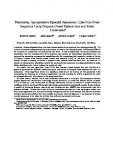
Fig. 1. A two-input, two-output conveyor system. Packages enter via one of the inputs I1 or I2 and leave the system via one of the outputs as illustrated. The system is composed using instances of Segments and Turns [3, 21].

5.1.1. Conveyor System Material handling conveyor systems move packages or material units from one or more inputs to specified outputs along predetermined paths. Such systems are used extensively in manufacturing, packaging, packet sorting etc. A typical conveyor system with two inputs and two outputs is shown in Fig. 1. This system is composed using instances of Segment and Turn units that each operate autonomously. A Segment moves a package over a predetermined length over its belt. A Turn is a unit that can serve as a merger or splitter for package flow. Each segment and turn unit has a predetermined maximum speed of operation and each unit has local sensors and actuators that are used to autonomously control its local behavior. The simulator we used produces a detailed event-trace of every change of state (event) in the sensors and actuators of each unit as packages move through the system. The movement of the packages in the conveyor system is transformed to a temporal sequence as follows. We label the exit points of each input, output, turn and segment. We consider the transfer of a package from one conveyor unit to another as an event. The unit represents the type of the event and the time at which each event occurs is recorded as the event time. Hence, when a package moves along a path, an ordered sequence of events is recorded. All the events corresponding to one package may not be contiguous because during the same time other packages may be moving along other paths. We consider three conveyor system datasets coming from three different topologies. Each topology can be identified by the various paths from the inputs to the outputs and the package input rates. We consider the package input arrival rates to be Poisson. The details of the three datasets is given in Table 3 and the structure of the topologies are given in Figures 1, 2 and 3. For the conveyor system data, there is only one data sequence corresponding to each topology. The GoKrimp algorithm works using a statistical dependency test called SignT est, which does not work on single sequence datasets. The implementation of GoKrimp asks such sequences to be broken into a number smaller sequences. Hence, the datasets were broken into sequences of size 25, 50 and 100 respectively for the 2I-2O, 3I-3O and the Package Sorter Topologies (creating longer sizes for sequences with longer and higher number of paths). Also, the conveyor system datasets are time stamped datasets. The SQS and

Discovering Compressing Serial Episodes from Event Sequences

19

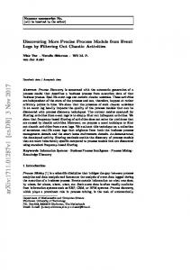
Fig. 2. Three-input, three-output conveyor system.

Fig. 3. Package Sorter topology. Table 3. Various Conveyor system topologies, input rates, alphabet size M , number of events (in the final data set with the topology) and the paths in each topology. Topology

InputRate (Poisson)

M

Events

Paths

2I-2O

0.6

16

7659

P1. I1 S1 T1 S4 T3 S7 T4 S8 O2 P2. I2 S6 T3 S7 T4 S5 T2 S3 O1

3I-3O

0.4

33

12497

P1. I1 S1 T1 S4 T3 S12 T7 S16 T8 S17 T9 S18 O3 P2. I2 S6 T3 S7 T4 S5 T2 S3 T5 S9 O1 P3. I3 S15 T7 S16 T8 S17 T9 S14 T6 S11 O2

Package Sorter

0.2

64

18489

P1. P2. P3. P4. P5.

I1 I2 I3 I4 I5

S39 T13 S32 S33 S34 T14 S28 S25 S22 T8 S19 T9 S20 T10 S21 T11 S24 T12 S27 O2 S31 T13 S32 S33 S34 T14 S35 T15 S36 S37 S38 T16 S40 O3 S16 T6 S17 T7 S13 T3 S5 S6 S7 S8 S9 T4 S10 T5 S11 O1 S2 T1 S3 T2 S4 T3 S5 S6 S7 S8 S9 T4 S10 T5 S15 T11 S24 T12 S27 O2 S1 T1 S3 T2 S12 T6 S17 T7 S18 T8 S19 T9 S23 S26 S29 T15 S36 S37 S38 T16 S40 O3

20

Ibrahim. A et al

Table 4. Patterns discovered by various algorithm in the Conveyor System data sets. The patterns for the CSC-2 is shown without the inter event gap. PS stands for Package Sorter. Method GOKRIMP

SQS

Topology

Top Discovered Patterns

2I-2O 3I-3O PS

[ S8 T4 S4 S2 T1 ], [ T3 I2 S3 S6 ], [ I1 O2 S8 ], [ S6 S4 S7 S5 ], [ S2 T1 S1 ], [ S8 T4 S4 ] [ T5 T9 ], [ S10 I1 S14 ], [ S2 T1 ], [ T3 T6 S18 ], [ S16 S12 ], [ S8 S6 ] [ T2 S4 ], [ S27 O2 ], [ S10 S12 ], [ S17 S18 ], [ S19 T10 ], [ S34 S35 ]

2I-2O

[S3 S8 T2 S7 T4 T3 S6 I2 O1 O2 T4], [O1 S8 T4], [O1 S8 T2 T4], [S3 S8 T2 T4 T3 S6 I2 O1 O2], [T4 T3 S6][S5 S7 T4 T3] [T6 T9], [O2 S18], [O1 S11], [O3 S9], [T8 T7 S7], [T7 T3] [T16 S24 ], [S15 S36 ], [T11 S36 ], [T5 S24 ], [T10 T15 ], [S21 S36 ], [T12 S38 ]

3I-3O PS 2I-2O

CSC-2

3I-3O PS

[S6 T3 S7 T4 S5 T2 S3 O1], [S1 T1 S4 T3 S7 T4 S8 O2], [S4 T3 S7 T4 S8 O2] [I1 I2], [T3 S7 T4], [T1 I2] [S15 T7 S16 T8 S17 T9 S14 T6 S11 O2], [S6 T3 S7 T4 S5 T2 S3 T5 S9 O1] [S12 T7 S16 T8 S17 T9 S18 O3], [I1 S1 T1 T3 T7 S16 T8 S17 T9], [T7 S16 T8 S17 T9] [T3 S5 S6 S7 S8 S9 T4 S10 T5], [S12 T6 S17 T7 T8 S19 T9 S23 S26 T15 S36 S37 S38 T16 S40 O3] [S39 T13 S32 S33 S34 T14 S28 S25 T8 S19 T9 S20 T10 T11 S24 T12 S27 O2] [T15 S36 S37 S38 T16 S40 O3], [T13 S32 S33 S34 T14] [S16 T6 S17 T7 T3 S5 S6 S7 S8 S9 T4 S10 T5], [S1 T1 S3 T2 T6 S17 T7]

GoKrimp algorithms do not take time stamped data. Hence experiments for SQS and GoKrimp on these datasets is carried out after removing the time stamps, while retaining the temporal ordering of the symbols.

5.1.2. Interpretability of Selected Patterns on conveyor system dataset Since the Conveyor system dataset consists of movement of packages through specific paths, we expect the good patterns to be sub paths of these paths. The results on the three Conveyor system data sets is given in Table 4. In all the three data sequences, our algorithm retrieves episodes corresponding to the sub paths of package flow (see Table 3 for the actual paths). These patterns actually correspond to sub paths where the packages move along the segments and turns at a fixed speed, without any congestion. The patterns returned by SQS and GoKrimp did not have any particular significance with respect to the topologies. Even though SQS gave some long patterns, those did not give any information regarding the underlying system of transportation of packages.

5.1.3. Effectiveness and Efficiency of the Algorithms In this section, we compare the effectiveness and efficiency of the methods in terms of compression achieved, the number of patterns returned and the run time on the conveyor system data set. Since the other methods, GoKrimp and SQS, employ a bit level coding scheme, for comparison purpose, we also calculate the exact bits needed for our encoding scheme, even though it doesn’t affect the encoding efficiency as discussed earlier. The encoding scheme remains exactly the same except for the specification of the alphabet size M in the beginning of the encoding. Since we only deal with positive integers, we assume that all the positive integers are encoded using the Elias codes [13]. For a positive integer, n, the Elias Code Length for encoding n is 2blog2 (n)c + 1. Each event-type is

Discovering Compressing Serial Episodes from Event Sequences

21

Table 5. Compression achieved by various algorithms on conveyor system data sequences. Datasets

SQS

GoKrimp

CSC-2

CSC-2 (Bitwise)

2I-2O 3I-3O PackageSorter

1.42 1.13 1.04

1.36 1.11 1.015

4.56 4.63 3.34

4.79 4.89 3.6

Table 6. Number of Patterns returned by various algorithms on conveyor system data sequences. Datasets

SQS

GoKrimp

CSC-2

2I-2O 3I-3O PackageSorter

65 114 140

20 22 9

13 27 77

encoded using a fixed code size of blog M c + 1 bits. It is easy to see that this bit level encoding scheme can also be easily decoded as discussed earlier. For each method, the compression achieved is calculated as the ratio of size of encoded data using singleton patterns to the size of encoded data using the selected patterns returned by the methods. Table 5 shows the compression ratios achieved by the three algorithms on the conveyor system data sets. Here, the column CSC-2 lists compression ratio in terms of memory units, while the last column CSC-2(Bitwise) gives the bit level compression ratio for CSC-2. As can be seen, our compression ratio is better by a factor of 3. As mentioned earlier, remote visualization and monitoring of such composable conveyor system is a potential application area of temporal data mining where the compression achieved is also important. Our method achieves better compression and also returns a very relevant set of episodes. Table 6 shows the number of patterns returned by the three methods and Table 7 shows run times of the three methods. Ideally for datasets with some inherent regularity in the sequence, a few significant patterns should explain the dataset well. In such cases, a good method should return a few relevant patterns. For the conveyor system datasets, where there is inherent regularity in the form of packet flows, CSC-2 returns a few highly relevant patterns, which happen to be sub paths of packet flows. GoKrimp also returns a small number of patterns, though as seen in Table 4, they are not relevant episodes. The PackageSorter topology is a complex topology with lots of intersecting paths. Hence CSC-2 captures more number of patterns here than from other topologies. As shown in Table 4, the patterns corresponded to sub paths relevant to the topology. But for the same topology, GoKrimp gives the minimum number of patterns. However none of these patterns are relevant in the sense that they capture good regularities in the underlying system. Hence GoKrimp algorithm fails to even see any inherent regularity in the datasets (which is also seen by the low compression achieved). SQS returns the highest number of patterns in all cases, which are all but irrelevant to these topologies.

22

Ibrahim. A et al

Table 7. Run times in seconds on conveyor system data sequences. Datasets

SQS

GoKrimp

CSC-2

2I-2O 3I-3O PackageSorter

6 14 20

1 1 1

1 1 2

Table 8. Patterns discovered by various algorithm in the JMLR data. Method

Top Discovered Patterns

GOKRIMP

support vector machin real world machin learn data set bayesian network

state art high dimension reproduc hilbert space larg scale independ compon analysi

neural network experiment result sampl size supervis learn support vector

well known special case solv problem signific improv object function

SQS

support vector machin machin learn state art data set bayesian network

larg scale nearest neighbor decis tree neural network cross valid

featur select graphic model real world high dimension mutual inform

sampl size learn algorithm princip compon analysi logist regress model select

CSC-2

support vector machin data set learn algorithm machin learn bayesian network

reproduc kernel hilbert space real world model select featur select high dimension

classif problem optim problem loss function state art larg scale

experiment result gener error supervis learn graphic model propos method

5.2. Results on other data sets We now discuss the experimental results on the datasets given in Table 2. We first show the interpretability of the patterns output by different methods on the JMLR data. In section 5.2.2, we compare the methods for efficiency in terms of compression achieved, runtime and the number of patterns. In section 5.2.3, the effectiveness of the selected patterns from different methods is analyzed using the patterns as features for classification.

5.2.1. Interpretability of Selected Patterns Of the six real world data sets, only the outputs from the JMLR data could be analyzed for interpretability. For the JMLR data set, we expect key phrases relevant to Machine Learning Research to pop up. We ran the CSC-2 algorithm with K = 20 to find the top 20 selected patterns. For the other two algorithms we just selected the top 20 of the outputted patterns. Table 8 gives the patterns obtained on JMLR text data. As can be seen, the patterns returned by all three of the methods are relevant and almost identical. Also we couldn’t see any redundancy in any of the pattern sets.

5.2.2. Efficiency of the algorithms In this section, we analyze the efficiency of the methods in terms of compression achieved, the number of patterns returned and the run time on the data sets listed in Table 2. Table 9 presents the comparison of compression ratio for different methods. Again, the column named CSC-2 lists compression ratio in terms

Discovering Compressing Serial Episodes from Event Sequences

23

Table 9. Compression achieved by various algorithms. Datasets

SQS

GoKrimp

CSC-2

CSC-2 (Bitwise)

jmlr aslbu aslgt auslan2 context pioneer

1.039 1.155 1.308 1.571 2.7 1.3

1.008 1.123 1.156 1.428 1.7 1.17

1.07 1.17 1.98 1.88 1.95 1.58

1.117 1.24 1.99 1.96 1.98 1.74

Table 10. Number of Patterns returned by various algorithms. Datasets

SQS

GoKrimp

CSC-2

jmlr aslbu aslgt auslan2 context pioneer

580 195 1095 13 138 143

20 67 68 4 33 49

765 453 105 7 39 134

of memory units and the last column, CSC-2(Bitwise), gives the bit level compression ratio for CSC-2. As is seen in Table 9, CSC-2 offers better compression on almost all the datasets. Table 10 shows the number of patterns returned by the three methods on real data. For the JMLR data, GoKrimp extracted only 20 patterns, which as we showed in Table 8, are all relevant. For SQS and CSC-2, the number of selected patterns were quite large. The initial phrases were all relevant to machine learning, as seen in Table 8. Later on, for the CSC-2 algorithm, most of the patterns returned were either relevant or slightly relevant machine learning, optimization and mathematical phrases with a bit of redundancy between the phrases. Never the less, we could make some sense out of most of the returned phrases. For the rest of the data sets, the size of the selected set of CSC-2 is in between that of the GoKrimp and SQS methods. We would like to point that the size of the selected set as such, without considering the relevance of the selected patterns does not have any particular significance. In Section 5.2.3, we discuss this again in relation to classification accuracy. Table 11 compares the run times. Except for the JMLR text data, our method took less than 2s for all the other data sets. For the JMLR data, the number of event types M is high (see Table 2) and hence the candidate set C for CSC-2 is high, which results in more time for calculating the OM matrix. On the data set aslgt, both SQS and GoKrimp take a lot of time because the number of events in the sequence is very large. However this does not affect our method much.

5.2.3. Classification Results Here we show the classification results on the five labeled datasets in Table 2 (The JMLR data has no class labels). For each method, we select class specific patterns using the respective methods and merge them along with the set of all singletons (which are 1-node episodes) to form features/attributes for classification. Thus, for classification, each sequence is represented by a feature vector consisting of the number of occurrences of each of the (selected) patterns together with the counts

24

Ibrahim. A et al

Table 11. Run times in seconds. Datasets

SQS

GoKrimp

CSC-2

jmlr aslbu aslgt auslan2 context pioneer

489 196 > 10Hrs 1 70 10

2 28 1440 1 36 6

182 5 4 1 1 1

Table 12. Percentage Classification accuracy achieved by various algorithms on 20 runs. Datasets

SQS Accuracy Mean σ

GoKrimp Accuracy Mean σ

CSC-2 Accuracy Mean σ

CSC-2∗ Accuracy Mean σ

Singletons Accuracy Mean σ

aslbu aslgt auslan2 context pioneer

70.08 86.12 35 94.02 100

68.57 85.55 32.7 93.83 100

70.02 85.9 35.18 93.7 100

71.15 86.1 34.05 94 100

69.7 82.17 32.58 94.02 100

0.68 0.18 1.23 0.94 0

0.83 0.23 1.6 0.61 0

0.94 0.15 1.2 0.89 0

0.75 0.19 1.13 0.65 0

1.1 0.19 1.7 0.58 0

of the singletons in the sequence . We also show the results, when only singletons are used as features. We call this method as Singletons in the tables. In [13], GoKrimp was compared with closed mining episode method, BIDE [25], and one of their two step (mining and then subset selection) methods, SEQKrimp [12,13]. They used different classifiers and found that the linear SVM classifier was giving the best results for almost all datasets. And for all the datasets, they showed that the top patterns returned by the SeqKrimp and GoKrimp were giving better classification accuracy than the top patterns returned by the BIDE algorithm. For our study, we thus use the linear SVM as the classifier using the libsvm package [8]. Since SeqKrimp and GoKrimp were giving similar results, we only use GoKrimp for this comparison study as SeqKrimp is computationally very intensive. The fixed interval serial episode patterns returned by CSC-2 are used as features in two different ways. In the first method, features are the counts of the selected fixed interval serial episodes along with the counts of the singletons. In the second approach, we drop the fixed inter-event constraints from the episodes and treat them as normal serial episodes (and care is taken to avoid multiple representations of the same serial episode). The counts of these serial episodes along with the singleton counts would be the feature representation of the sequences. The first method is called as CSC-2 and the second method is called CSC-2∗ in the results table. For each dataset, the results were obtained by averaging 20 repetitions of 10-fold cross-validation. The results are shown in Table 12. The table gives the mean and standard deviation (σ) of the classification accuracy. We see that, SQS marginally outperforms the other methods for the aslgt and context datasets and the two CSC-2 methods have higher accuracies for the aslbu and auslan2 data sets, respectively. In all the datasets, however, the accuracies are similar for SQS and CSC-2. In comparison, the accuracies of the GoKrimp method are slightly lower than both the SQS and CSC-2 methods, except for the pioneer data, where none of the methods seem to misclassify. Table 13 shows the number of patterns

Discovering Compressing Serial Episodes from Event Sequences

25

Table 13. The average number of features per data set for each method. The number (except for the Singletons) is the number of non-singleton extracted patterns which represent the feature set along with the singletons. Datasets

SQS

GoKrimp

CSC-2

Singletons

aslbu aslgt auslan2 context pioneer

70 1154 15 150 132

17 418 0 64 24

23 923 6 42 121

263 94 23 107 184

selected by each method as features and we see that the number of features selected by SQS is far higher than other methods. And we noticed that, even though the performance of SQS was only slightly better than CSC-2, the run time for the experiments was at least five times longer than that of CSC-2. On the other hand, GoKrimp selects comparatively the lowest number of patterns (except for the context data set) and also has the lowest accuracy among the three methods. For the auslan2 dataset, GoKrimp couldn’t extract any pattern and hence the classification accuracy is similar to Singletons (the slight difference is due to difference in the Cross Validation splits for different runs). It is also interesting to see that the Singletons method, which consists of only the 1-node counts are always close to the best results. But nevertheless, the table shows that the selected patterns from different methods have contributed to the increase in accuracy.

5.3. Discussion The results presented here show that CSC-2 is a good method for finding a subset of patterns that achieve good compression. It is also seen that these patterns that achieve good compression are also highly relevant for the problem. For the conveyor system datasets, our method was shown to perform extremely well in pulling out patterns representing the stable flow of items and achieving great compression. Both the aspects are of great importance for remote monitoring of such systems as discussed earlier. The other methods have failed in doing so. On these datasets, the other algorithms, namely SQS and GoKrimp failed to find patterns that capture the package flow and they also could not achieve much data compression. We have also tested out method on some real world data sets. The CSC-2 algorithm discovered subsets of episodes that result in better data compression compared to the other methods and our algorithm also seems faster than other algorithms for most of the datasets. The subset of patterns identified by CSC-2 is also seen to be very effective in classification scenarios. Recall that the patterns used by CSC-2 are fixed interval serial episodes. Such episodes, as we have seen, suited the conveyor system data sets, where sequential occurrences of events follow such a fixed gap mechanism. For the other sequential datasets used for classification, such constraints may not be really relevant. But even on these data sets, CSC-2 identifies a subset of patterns that result in both data compression as well as better performance in classification. This shows that our pattern structure is not particularly restrictive and it is useful on a variety of data sets.

26

Ibrahim. A et al

6. Conclusion Frequent episodes discovered from sequential data are supposed to give us good insights into the characteristics of the data source. However, in practice, most mining algorithms output a large number of highly redundant episodes. Isolating a small subset of episodes that succinctly characterize the data is a challenging problem. In this paper, we presented an MDL based approach for this problem. Using the interesting class of fixed interval serial episodes and a novel data encoding scheme, we presented a method to discover a subset of highly relevant episodes. In contrast to methods in [12, 13, 23], our method achieves good data compression, while being able to work with event sequences with time stamps. We compared our method with SQS and GoKrimp on text data and also on a number of real world data sets which were used earlier in temporal data mining. On all these data sets, our method is good in comparison to others, both in terms of compression and run time. For the classification scenario, our method was only slightly less effective than SQS but better than GoKrimp. But we achieved it with far fewer patterns and very low run times. In this paper, we also briefly discussed a novel application area for sequential pattern mining. This is the composable conveyor system. We presented empirical comparison of our method with that of others on three data sets from this problem domain to demonstrate both the effectiveness and efficiency of our method. In this paper, we have not attempted any statistical analysis of our method so that we can relate the data compression to some measure of statistical significance of the pattern subset isolated by our method. This is an interesting and challenging direction to extend the work presented here. We would be exploring this in our future work.

References [1] A. Achar, A. Ibrahim, and P. S. Sastry. Pattern-growth based frequent serial episode discovery. Data & Knowledge Engineering, 87:91–108, 2013. [2] A. Achar, S. Laxman, and P. S. Sastry. A unified view of the apriori-based algorithms for frequent episode discovery. Knowledge and information systems, 31(2):223–250, 2012. [3] B. Archer, S. Shivakumar, A. Rowe, and R. Rajkumar. Profiling primitives of networked embedded automation. In Automation Science and Engineering, 2009. CASE 2009. IEEE International Conference on, pages 531–536. IEEE, 2009. [4] D. Burdick, M. Calimlim, J. Flannick, J. Gehrke, and T. Yiu. Mafia: A maximal frequent itemset algorithm. Knowledge and Data Engineering, IEEE Transactions on, 17(11):1490– 1504, 2005. [5] T. Calders and B. Goethals. Mining all non-derivable frequent itemsets. In Principles of Data Mining and Knowledge Discovery, pages 74–86. Springer, 2002. [6] G. Casas-Garriga. Summarizing sequential data with closed partial orders. In SDM, volume 5, pages 380–391. SIAM, 2005. [7] V. Chandola and V. Kumar. Summarization–compressing data into an informative representation. Knowledge and Information Systems, 12(3):355–378, 2007. [8] C.-C. Chang and C.-J. Lin. LIBSVM: A library for support vector machines. ACM Transactions on Intelligent Systems and Technology, 2:27:1–27:27, 2011. Software available at http://www.csie.ntu.edu.tw/~cjlin/libsvm. [9] F. Geerts, B. Goethals, and T. Mielik¨ ainen. Tiling databases. In Discovery science, pages 278–289. Springer, 2004. [10]P. D. Gr¨ unwald. The minimum description length principle. The MIT Press, 2007. [11]J. Han, H. Cheng, D. Xin, and X. Yan. Frequent pattern mining: current status and future directions. Data Mining and Knowledge Discovery, 15(1):55–86, 2007.

Discovering Compressing Serial Episodes from Event Sequences

27

[12]H. T. Lam, F. M¨ orchen, D. Fradkin, and T. Calders. Mining compressing sequential patterns. In SDM, pages 319–330. SIAM, 2012. [13]H. T. Lam, F. M¨ orchen, D. Fradkin, and T. Calders. Mining compressing sequential patterns. Statistical Analysis and Data Mining, 7(1):34–52, 2014. [14]S. Laxman, P. S. Sastry, and K. P. Unnikrishnan. A fast algorithm for finding frequent episodes in event streams. In Proceedings of the 13th ACM SIGKDD international conference on Knowledge discovery and data mining, pages 410–419. ACM, 2007. [15]D.-I. Lin and Z. M. Kedem. Pincer-search: an efficient algorithm for discovering the maximum frequent set. Knowledge and Data Engineering, IEEE Transactions on, 14(3):553– 566, 2002. [16]H. Mannila, H. Toivonen, and A. I. Verkamo. Discovery of frequent episodes in event sequences. Data Mining and Knowledge Discovery, 1(3):259–289, 1997. [17]N. M´ eger and C. Rigotti. Constraint-based mining of episode rules and optimal window sizes. Knowledge Discovery in Databases: PKDD 2004, pages 313–324, 2004. [18]F. Moerchen and D. Fradkin. Robust mining of time intervals with semi-interval partial order patterns. In SDM, pages 315–326. SIAM, 2010. [19]N. Pasquier, Y. Bastide, R. Taouil, and L. Lakhal. Discovering frequent closed itemsets for association rules. In Database Theory—ICDT’99, pages 398–416. Springer, 1999. [20]J. Rissanen. A universal prior for integers and estimation by minimum description length. The Annals of statistics, pages 416–431, 1983. [21]S. Shivakumar. Sensor-actuator systems for automation. In Work In Progress Session, IEEE Real-time Systems Symposium. IEEE, 2006. [22]A. Siebes, J. Vreeken, and M. van Leeuwen. Item sets that compress. In SDM, volume 6, pages 393–404. SIAM, 2006. [23]N. Tatti and J. Vreeken. The long and the short of it: Summarising event sequences with serial episodes. In Proceedings of the 18th ACM SIGKDD international conference on Knowledge discovery and data mining, pages 462–470. ACM, 2012. [24]J. Vreeken, M. Van Leeuwen, and A. Siebes. Krimp: mining itemsets that compress. Data Mining and Knowledge Discovery, 23(1):169–214, 2011. [25]J. Wang and J. Han. Bide: Efficient mining of frequent closed sequences. In Data Engineering, 2004. Proceedings. 20th International Conference on, pages 79–90. IEEE, 2004. [26]J. Wang, J. Han, and J. Pei. Closet+: Searching for the best strategies for mining frequent closed itemsets. In Proceedings of the ninth ACM SIGKDD international conference on Knowledge discovery and data mining, pages 236–245. ACM, 2003. [27]J. Wang and G. Karypis. On efficiently summarizing categorical databases. Knowledge and Information Systems, 9(1):19–37, 2006. [28]I. H. Witten, A. Moffat, and T. C. Bell. Managing gigabytes: compressing and indexing documents and images. Morgan Kaufmann, 1999. [29]Y. Xiang, R. Jin, D. Fuhry, and F. F. Dragan. Succinct summarization of transactional databases: an overlapped hyperrectangle scheme. In Proceedings of the 14th ACM SIGKDD international conference on Knowledge discovery and data mining, pages 758–766. ACM, 2008. [30]X. Yan, J. Han, and R. Afshar. Clospan: Mining closed sequential patterns in large datasets. In Proceedings of SIAM International Conference on Data Mining, pages 166–177. SIAM, 2003.