Process Model Discovery: A Method Based on Transition System Decomposition? Anna A. Kalenkova1 , Irina A. Lomazova1 , and Wil M.P. van der Aalst1,2 1
National Research University Higher School of Economics (HSE), Moscow, 101000, Russia {akalenkova,ilomazova}@hse.ru 2 Eindhoven University of Technology, P.O. Box 513, NL-5600 MB, Eindhoven, The Netherlands
[email protected]
Abstract. Process mining aims to discover and analyze processes by extracting information from event logs. Process mining discovery algorithms deal with large data sets to learn automatically process models. As more event data become available there is the desire to learn larger and more complex process models. To tackle problems related to the readability of the resulting model and to ensure tractability, various decomposition methods have been proposed. This paper presents a novel decomposition approach for discovering more readable models from event logs on the basis of a priori knowledge about the event log structure: regular and special cases of the process execution are treated separately. The transition system, corresponding to a given event log, is decomposed into a regular part and a specific part. Then one of the known discovery algorithms is applied to both parts, and finally these models are combined into a single process model. It is proven, that the structural and behavioral properties of submodels are inherited by the unified process model. The proposed discovery algorithm is illustrated using a running example.
1
Introduction
Process mining techniques can be used, amongst others, to discover process models (e.g., in the form of Petri nets) from event logs. Many discovery methods were suggested in order to obtain process models reflecting a behavior presented in event logs. Discovered process models may vary considerably depending on a chosen discovery method. For an overview of process discovery approaches and techniques see [15]. The main challenge of process discovery is to construct an adequate formal model reflecting behavior presented in an event log in a best possible way. Quality criteria for process models discovered from event logs are described in [2]. The first criterion is (replay) fitness: a process model should allow for behavior recorded in an event log. The next one is precision: a discovered process model ?
This work is supported by the Basic Research Program of the National Research University Higher School of Economics.
should not allow for behavior which differs markedly from an event log records (no underfitting). The generalization criterion states that a discovered model should be general enough (no overfitting). And the last but not least quality criterion is simplicity: a discovered model should not be too complicate and confusing. In this paper we focus on simplicity, fitness and precision. The goal of our work is to present a decomposition method for obtaining clearer and simpler models, trying to preserve their fitness and precision. The decomposition method proposed in this paper aim to exploit modularity in processes to obtain more readable process models. For other quality metrics for evaluation of simplicity see [22]. Most of process mining algorithms for discovering a model from an event log first build a (labeled) transition system from an event log, and then use different techniques to construct a model from this transition system. We also follow this approach. Methods for building transition systems based on event logs were proposed in [6] and are out of the scope of this paper. In this paper we assume that there is a transition system, already constructed from some event log, and concentrate on discovering a process model from a given transition system. Moreover, we assume that a transition system is decomposed into a regular and specific parts on base of some a priori knowledge about a modeled system. For each of the parts we apply existing process discovery algorithms to obtain corresponding (sub)process models. Then these models are combined into a single process model. For discovering subprocess models we suggest to use state-based region algorithms and algorithms based on regions of languages. The state-based region approach was initially proposed by A. Ehrenfeucht and G. Rozenberg [16]. Later this approach was generalized by J. Cortadella et al. [12, 13]. An alternative generalization was proposed by J. Carmona et al. [11]. The application of statebased region algorithms to process mining was studied in [6, 9, 21]. Algorithms based on regions of languages were presented in [7, 14, 18] and then applied to process mining [8, 24]. State-based region algorithms and algorithms based on regions of languages map discovered regions into places of a target Petri net. The advantage of these algorithms is that they guarantee “perfect” fitness, i.e. every trace in a log (a transition system) can be reproduced in a model. However, a large degree of concurrency in a system and incompleteness of an event log (or corresponding transition system) may lead to a blowup of the diagram comparable to the the state explosion problem. The paper is organized as follows. In Section 2 a motivating example is presented. Section 3 introduces basic definitions and notions, including traces, Petri nets and transition systems. In Section 4 we propose a decomposition algorithm for constructing a process model. In Section 5 we formally prove that the structural and behavioral properties of subprocess models constructed from the decomposed transition system are inherited by the unified process model. Section 6 presents related work. Section 7 concludes the paper.
2
Motivating Example
In this section we will consider booking a flight process. The log reflecting a history of process execution is presented in Fig. 1. The transition system constructed from this log is depicted in Fig. 2. L = {hstart booking, book f light, get insurance, send email, choose payment type, pay by card, complite bookingi, hstart booking, get insurance, book f light, send email, choose payment type, pay by card, complite bookingi, hstart booking, get insurance, book f light, send email, choose payment type, pay by web money, complite bookingi, hstart booking, book f light, get insurance, send email, choose payment type, pay by web money, complite bookingi, hstart booking, book f light, cancel, send emaili, hstart booking, book f light, get insurance, send email, choose payment type, hcancel, send emaili}. Fig. 1. An event log for a booking process
s1 start_booking
s2 book_flight
get_insurance
s3
s4
get_insurance book_flight cancel
s5 send_email
s6 choose_payment_type s7 cancel pay_by_card
s9
s8 pay_by_web_money
complite_booking send_email
s10
Fig. 2. A transition system for a booking process constructed from the event log depicted in Fig. 1
At the beginning of a booking process a customer needs to book a flight and to get an insurance, these actions are performed in parallel.
Then an email is sent to confirm the booking. After that the customer chooses a payment method, pays and the booking process successfully completes. If the booking was cancelled, an email is sent to notify the cancellation. These cancellations may occur during an execution of booking procedures as well as after the booking was accepted. Let us consider the models produced by the standard state-based region algorithm1 (Fig. 3) and the language-based synthesis algorithm2 (Fig. 4) from original transition system and corresponding event log respectively. book_flight
pay_by_card
choose_payment_type pay_by_web_money start_booking cancel get_insurance complete_booking
send_email
Fig. 3. The result of applying the standard state-based region algorithm to the transition system depicted in Fig. 2 pay_by_card
pay_by_web_money complete_booking start_booking
cancel
send_email
book_flight get_insurance
choose_payment_type
Fig. 4. The result of applying the language-based synthesis algorithm to the event log depicted in Fig. 1 1
2
The State-based regions Miner plug-in is available in Prom framework [23]. This plug-in implements the standard state-based region algorithm presented in [12, 13]. The ILP Miner [24] plug-in is implemented in Prom framework [23]. We choose such parameters that there are no tokens left after a case completion, and initial places don’t have incoming arcs.
Figures 3 and 4 illustrate that region-based techniques may result in models that are more complicated than the corresponding transition system. In this paper we present a method for discovering better structured and more readable process models by detecting a regular behavior in a given transition system. We split a transition system in two parts: one of them represents a regular behavior, and the other describes handling special cases (exceptions, cancellations, etc.)
3
Preliminaries: Petri Nets and Transition Systems
Let S be a finite set. A multiset m over a set S is a mapping m : S → Nat, where Nat is the set of natural numbers (including zero), i.e. a multiset may contain several copies of the same element. For two multisets m, m0 we write m ⊆ m0 iff ∀s ∈ S : m(s) ≤ m0 (s) (the inclusion relation). The sum of two multisets m and m0 is defined as usual: ∀s ∈ S : (m + m0 )(s) = m(s) + m0 (s), the difference is a partial function: ∀s ∈ S such that m(s) ≥ m(s0 ) : (m − m0 )(s) = m(s) − m0 (s). By M(S) we denote the set of all finite multisets over S. Let S and E be two disjoint non-empty sets of states and events, and B ⊆ S × E × S be a transition relation. A transition system is a tuple TS = (S, E, B, sin , Sfin ), where sin ∈ S is an initial state and Sfin ⊆ S — a set of final e states. Elements of B are called transitions. We write s → s0 , when (s, e, s0 ) ∈ B. 0 A state s is reachable from a state s iff there is a possibly empty sequence ∗ of transitions leading from s to s0 (denoted by s → s0 ). A transition system must satisfy the following basic axioms: ∗
1. every state is reachable from the initial state: ∀s ∈ S : sin → s; 2. for every state there is a final state, which is reachable from it: ∀s ∈ S ∃sfin ∈ ∗ Sfin : s → sfin ; Let E be a set of events. A trace σ (over E) is a sequence of events, i.e., σ ∈ E ∗ . An event log L is a multiset of traces, i.e., L ∈ M(E ∗ ). A trace σ = he1 , . . . , en i is called feasible in a transition system TS iff e1 e2 en ∃s1 , . . . , sn−1 , sn ∈ S : sin → s1 → . . . sn−1 → sn , and sn ∈ Sfin , i.e. a feasible trace leads from the initial state to some final state. A language accepted by TS is defined as the set of all traces feasible in TS, and is denoted by L(TS). We say that a transition system TS and an event log L are matched iff each trace from L is a feasible trace in TS, and inversely each feasible trace in TS belongs to L. Let P and T be two finite disjoint sets of places and transitions, and F ⊆ (P × T ) ∪ (T × P ) — a flow relation. Let also E be a finite set of events, and λ : T → E be a labeling function. Then N = (P, T, F, λ) is a (labeled) Petri net. A marking in a Petri net is a multiset over the set of places. A marked Petri net (N, m0 ) is a Petri net together with its initial marking.
Pictorially, places are represented by circles, transitions by boxes, and the flow relation F by directed arcs. Places may carry tokens represented by filled circles. A current marking m is designated by putting m(p) tokens into each place p ∈ P . For a transition t ∈ T an arc (x, t) is called an input arc, and an arc (t, x) — an output arc; the preset • t and the postset t• are defined as the multisets over P such that • t(p) = 1, if (p, t) ∈ F , otherwise • t(p) = 0, and t• (p) = 1 if (t, p) ∈ F , otherwise t• (p) = 0. Note that we will also consider presets and postsets as sets of places. A transition t ∈ T is enabled in a marking m iff • t ⊆ m. An enabled transition t may fire yielding a new marking m0 =def m − • t + t• t
λ(t)
(denoted m → m0 , m → m0 , or just m → m0 ). We say that m0 is reachable from m iff there is a (possibly empty) sequence of firings m = m1 → · · · → mn = m0 . R(N, m) denotes the set of all markings reachable in N from the marking m. A marked Petri net (N, m0 ), N = (P, T, F, λ) is called safe iff ∀p ∈ P ∀m ∈ R(N, m0 ) : m(p) ≤ 1, i.e. at most one token can appear in a place. A reachability graph for a marked Petri net (N, m0 ) labeled with events from E is a transition system TS = (S, E, B, sin , Sfin ), with the set of states S = R(N, m0 ), the event set E, and transition relation B defined by (m, e, m0 ) ∈ B t iff m → m0 , where e = λ(t). The initial state in TS is the initial marking m0 . If some reachable markings in (N, m0 ) are distinguished as final markings, they are defined as final elements in TS. Note that TS may also contain other final states, to satisfy the axiom that for every state in TS there is a final state, which is reachable from it. Workflow nets (WF-nets) [1] is a special subclass of Petri nets designed for modeling workflow processes. A workflow net has one initial and one final place, and every place or transition in it is on a directed path from the initial to the final place. A (labeled) Petri net N is called a (labeled) workflow net (WF-net) iff 1. There is one source place i ∈ P and one sink place f ∈ P s. t. i has no input arcs and f has no output arcs. 2. Every node from P ∪ T is on a path from i to f . 3. The initial marking in N contains the only token in its source place. We denote by [i] the initial marking in a WF-net N . Similarly, we use [f ] to denote the final marking in a WF-net N , defined as a marking containing the only token in the sink place f . A WF-net N with an initial marking [i] and a final marking [f ] is sound iff 1. For every state m reachable in N , there exists a firing sequence leading from ∗ ∗ m to the final state [f ]. Formally, ∀m : [([i] → m) implies (m → [f ])]; 2. The state [f ] is the only state reachable from [i] in N with at least one token ∗ in place f . Formally, ∀m : [([i] → m) ∧ ([f ] ⊆ m) implies (m = [f ])]; ∗
λ(t)
3. There are no dead transitions in N . Formally, ∀t ∈ T ∃m, m0 : (i → m → m0 ).
4
Method for Constructing Structured and Readable Process Models
As shown by the example in the Section 2 straightforward application of the synthesis algorithms may give rather confounded process models. Prior knowledge of a modular process structure can be used to identify subprocesses and clarify the target process model. Our goal is to construct readable process models which will reflect modular structures of processes. 4.1
Decomposition of a Transition System
Assume that we can identify a regular and a special process behavior within the original transition system. Let us consider a transition system TS = (S, E, B, sin , Sfin ) and divide the set of states into two non-overlapping subsets which correspond to a regular and a special behavior: S = Sreg ∪ Sspec , Sreg ∩ Sspec = ∅ (Fig. 5). Let Breg denote a
Besc
Sreg
Sspec
Breg Bspec
Bret
Fig. 5. Decomposition of a transition system
set of regular process transitions, Bspec denote a set of special transitions, Besc and Bret stand for transitions, which indicate escaping from the regular process flow and returning to the regular process flow respectively. Let Ereg and Espec
denote the set of events corresponding to Breg and Bspec respectively. Note that Ereg and Espec are not necessarily disjoint sets, i.e. the same label can appear in different parts of the transition system. Formally, set of states S can be partitioned over Sreg and Sspec and then the tuple TSdec = (TS, Sreg , Sspec ) is called a decomposed transition system if the following additional conditions hold: sin ∈ Sreg and Sfin ⊆ Sreg . The construction of such a transition system from an event log can be performed in two steps. Firstly, a transition system is constructed for the traces corresponding to a regular process behavior. Secondly, an additional behavior is added to the transition system, and new states are marked as special. 4.2
Region-Based Algorithms
An algorithm for synthesis of a marked Petri net from a decomposed transition system will be build on well-known region based algorithms. Therefore, we will give an overview of these algorithms and outline their properties, which will be used in the further analysis of the presented algorithm. State-based region algorithm First, we briefly describe the standard state-based region algorithm [12, 13]. Let TS = (S, E, T, sin , Sfin ) be a transition system and S 0 ⊆ S be a subset of states. S 0 is a region iff for each event e ∈ E one of the following conditions hods: e
– all the transitions s1 → s2 enter S 0 , i.e. s1 ∈ / S 0 and s2 ∈ S 0 , e 0 – all the transitions s1 → s2 exit S , i.e. s1 ∈ S 0 and s2 ∈ / S0, e 0 – all the transitions s1 → s2 do not cross S , i.e. s1 , s2 ∈ S 0 or s1 , s2 ∈ / S0. A region r0 is said to be a subregion of a region r iff r0 ⊆ r. A region r is called a minimal region iff it does not have any other subregions. The state-based region algorithm constructs a target Petri net in such a way that a transition system is covered by its minimal regions and after that every minimal region is transformed to a place in the Petri net. The result of applying the standard state-based region algorithm to the transition system which corresponds to a regular behavior of the booking process is presented in Fig. 6. Note that states in the transition system correspond to markings of the target Petri net. Let us enumerate the properties of the standard state-based region algorithm [12, 13], which will be used for the analysis of the discovery algorithm presented in this paper: 1. Every Petri net transition t ∈ T corresponds to an event in the initial transition system e ∈ E (the transition t is labeled with e), the opposite is not true (events of the initial transition system might be split). 2. There is a bisimulation between a transition system and a reachability graph of the target Petri net, this implies that every state in TS corresponds to a Petri net marking.
start_booking book_flight
start_booking
get_insurance book_flight
get_insurance
get_insurance book_flight send_email send_email choose_payment_type
choose_payment_type pay_by_card
pay_by_card
pay_by_web_money
pay_by_web_money
complite_booking complete_booking
Fig. 6. Applying the state-based region algorithm to the transition system which corresponds to a regular behavior of the booking process
3. The target Petri net is safe, i.e. no more than one token can appear in a place.
An algorithm based on regions of languages The aim of the different algorithms based on regions of languages [8,24] is to construct a Petri net, which is able to reproduce a given language (herein we will consider a language accepted by an initial transition system), reducing undesirable behavior by adding places. Addition of such places will not allow for construction of a Petri net, e.g. the flower-model (Fig. 7), which generates all the words in a given alphabet. A e1 en
e2
...
Fig. 7. A flower model
(language-based) region is defined as a (2 |T | + 1)-tuple of {0, 1}, representing an initial marking and a number of tokens each transition consumes and produces in a place. Like in the previous approach each region corresponds to a place in a Petri net. Regions are defined as solutions of the linear inequation system, constructed for a given language. The algorithms based on regions of languages satisfy the following conditions: 1. There is a bijection between Petri net transitions T and events in the initial transition system E, such that every transition is labeled with a corresponding event. 2. There is a homomorphism ω from a transition system TS to the reachability graph RG of a target Petri net N , i.e. for every s ∈ S there is a corresponding node - ω(s) in RG (every state in TS has a corresponding N marking), e such that ω(sin ) = m0 and for every transition (s1 → s2 ) ∈ B there is an arc (ω(s1 ), ω(s2 )) in RG labeled with e. 3. The target Petri net is safe. We will add constraints to obtain elementary Petri nets, in which transitions can only fire when their output places are empty [24], this implies that we will get a safe Petri net. Let us refer to the state-based algorithms and the algorithms based on regions languages, which meet the specified requirements, simply as basic region algorithms. 4.3
Constructing Transition Systems
In this subsection we give a method for constructing two separate transition systems from a given decomposed transition system. Before applying basic region algorithms to parts of a decomposed transition system we have to be sure that these parts are transition systems as well, otherwise they should be repaired. Let TSdec = ((S, E, B, sin , Sfin ), Sreg , Sspec ) be a decomposed transition system. As we can see from the example (Fig. 5) the subgraph formed by vertices from Sreg and transitions from Breg may not define a transition system, since it contains states which are not on the path from the initial state to some final state, and should be repaired. A set of novel events E 0 and a set of transitions B 0 labeled with this events should be added to retrieve missing connections between Sreg states (see Fig. 8). For every pair of nodes from Sreg having a path between them with a starting transition from Besc , a destination transition from Bret , and containing exactly one transition from Besc , such that there is no path between these nodes within the graph (Sreg , Breg ), a novel event e0 ∈ E 0 and a novel transition b0 ∈ B 0 labeled with this event should be added. One can note that after this transformation every state is on the path from sin to sfin ∈ Sfin , and we get a transition system TSreg = (Sreg , Ereg ∪ E 0 , Breg ∪ B 0 , sin , Sfin ). The subgraph formed by vertices from Sspec and transitions from Bspec should be also repaired to form a transition system. As in the previous case each pair
si
Sspec estart e1''
Sreg
e1'
e2'' e2' e3'
eend
eend so
Fig. 8. Constructing transition systems, which correspond to subprocesses
of states connected only through external nodes should be connected directly via transitions labeled with novel events (see Fig. 8). Note that a path through the external nodes should not contain transitions added to repair the transition system constructed for a normal flow. Let B 00 denote the set of novel transitions, E 00 denote the set of corresponding events. In contrast to the transition system TSreg constructed for the normal process flow in the previous step an initial state si and a final state (state without outgoing transitions) so should be added. All states having incoming transitions from Besc , should be connected with si by incoming transitions labeled with a special event estart . Let us denote the set of these transitions by Bstart . Similarly, all states having outgoing transitions from Bret should be connected with so by outgoing transitions labeled with the event eend . The set of such transitions will be denoted by Bend . After these transformations every state lies on a path from sin to sfin ∈ Sfin , and, hence, we obtain a transition system TSspec = (Sspec ∪ {si , so } , Espec ∪ E 00 ∪ {estart , eend } , Bspec ∪ B 00 ∪ Bstart ∪ Bend , si , {so }). 4.4
Discovery Algorithm
This algorithm uses some basic region algorithm A. Algorithm [Discovery algorithm]. (Constructing a marked Petri net for a decomposed TS). Input: A decomposed transition system TSdec = ((S, E, B, sin , Sfin ), Sreg , Sspec ). Step 1: Construct two transition systems: TSreg = (Sreg , Ereg ∪E 0 , Breg ∪B 0 , sin , Sfin ) and TSspec = (Sspec ∪ {si } ∪ {so } , Espec ∪ E 00 ∪ {estart , eend } ,
Bspec ∪ B 00 ∪ Bstart ∪ Bend , si , {so }) form the decomposed transition system TSdec . Step 2: Apply algorithm A to retrieve a regular (Nreg ) and a special (Nspec ) process flow from TSreg and TSspec respectively. Step 3: Restore the connections between Nreg and Nspec to create a so-called a unified Petri net N : e
esc s0 ) ∈ Besc , s ∈ Sreg , s0 ∈ Sspec add a novel – For every transition (s → Petri net transition labeled with eesc (see Fig. 9). Connect this transition by incoming arcs with all the places p ∈ P , such that m(p) > 0, and by outgoing arcs with the places p0 ∈ P 0 , such that m0 (p0 ) > 0, where m and m0 are markings corresponding to s and s0 respectively. Similarly, transitions from Bret should be restored.
Nreg
Sreg
Sspec m'
s`
Nspec m'
m
m
s eesc
eesc eret
...
s''
... m''
...
eret m''
...
...
N
Fig. 9. A unified Petri net
– Delete the following nodes along with their incident arcs from the result Petri net: transitions with labels from E 0 and E 00 , all the transitions labeled with estart along with the places from their presets (if these places don’t have other output arcs), and all the transitions labeled with eend along with the places from their postsets (if these places don’t have output arcs). – Initial marking for the result Petri net N is defined as an initial marking of Nreg , label function of the result N is defined on the basis of Nreg and Nspec label functions.
Output: Marked Petri net N . Note that after partitioning of the initial transition system into two transitions systems (Step 1), each of the parts can be in turn divided into subsystems. After decomposition a discovery algorithm is applied to each part (Step 2) and required connections are restored within the entire model (Step 3).
start_booking
estart
book_flight
get_insurance
send_email cancel eend choose_payment_ type
cancel
pay_by_card
pay_by_web_money
send_email
complete_booking
Fig. 10. The result of applying the discovery algorithm to the original transition system
Let us consider the initial transition system presented in Fig. 2. Suppose that we will divide the set of states in the following manner: S = Sreg ∪ Sspec , Sreg = {s1 , s2 , s3 , s4 , s5 , s6 , s7 , s8 , s10 }, Sspec = {s9 }. A Petri net which is constructed for this decomposed transitions system according to the discovery algorithm is presented in Fig. 10. The subprocesses structures can be easily retrieved from this model. Note, that dashed nodes and arcs denote those parts which were deleted during an execution of the discovery algorithm. Now assume that, we decided to divide the set of states as follows: S = Sreg ∪ Sspec , Sreg = {s1 , s2 , s4 , s5 , s6 , s7 , s8 , s10 }, Sspec = {s3 , s9 }. The result of applying the discovery algorithm to the decomposed transition system is presented in Fig. 11. This example shows that the result depends on choosing a partition of
the set of states. Expert knowledge can help to find an appropriate partition. For example, names of events, which correspond to an irregular behavior, can be helpful for that. Note, that the models, presented in Fig. 10 and Fig. 11, can be constructed by both: the state-based region algorithm and the algorithm based on regions of languages, which meet the requirements, listed in Subsection 5.2, with the only difference, that the algorithm based on regions of languages doesn’t produce final place.
start_booking
estart book_flight
get_insurance
get_insurance book_flight cancel
send_email
cancel choose_payment_type
pay_by_card
pay_by_web _money
eend
send_email complete_booking
Fig. 11. The result of applying the discovery algorithm to the original transition system with different states partition
5
Structural and Behavioral Properties Preserved by Decomposed Discovery
In this section we will formally prove that the structural and behavioral properties of subprocess models constructed from a decomposed transition system are
inherited by the unified process model. As was mentioned earlier the discovery algorithm use some basic region algorithm. A basic region algorithm is a statebased region algorithm, which guarantees the bisimilarity relation between an initial transition system and a reachability graph of the target Petri net, or an algorithm based on regions of languages, for which there is a homomorphism from a transition system to a reachability graph of the target Petri net. Bisimularity relation defined by the state-based region algorithm specifies exactly one state in a reachability graph for each state in a transition system, in such a case bisimularity implies homomorphism. So, our decomposition approach can use any of basic region algorithms, provided this algorithm outputs a safe Perti net, and there is a homomorphism from an initial transition system to the reachability graph of the target Petri net. 5.1
Structural Properties
First, we will show that the Discovery algorithm preserve connectivity properties of subprocess models, i.e. nodes connected within the subprocess model, obtained on the Step 2 of the Discovery algorithm, will be connected within the unified model. Lemma 1 (Connectivity properties). If there is a directed path between a pair of nodes (i.e., places or transitions) within subprocess model Nreg (Nspec ) and these nodes were not deleted during the construction of the unified Petri net model N = (P, T, F, λ), then there is a directed path between them within N . Proof. Let TSdec = (TS, Sreg , Sspec ) be a decomposed transition system. Let us consider two arbitrary nodes u, v ∈ P 0 ∪ T 0 within Nreg = (P 0 , T 0 , F 0 , λreg ). By construction there is a path between them before the deletion of unnecessary nodes. Let us prove that u, v will be connected after the deletion as well. Consider transition t ∈ T 0 labeled with e0 , which should be deleted along with all incident arcs (see Fig. 12). Let us prove that the nodes from • t and t• are still connected with each other. If so, connection between arbitrary nodes u and v will be preserved. Consider e0
transition (s1 → s2 ), s1 , s2 ∈ Sreg , which was added to the transition system constructed for Sreg (see Fig. 12). Let Bspec , Besc , and Bret be transitions of the decomposed transition system, connecting nodes as it shown in Fig. 5. There is an alternative path within the transition system between s1 and s2 which contains transitions from Besc , Bspec and Bret . Since there is a homomorphism from the transition system to the reachability graph of the target Petri net, there is a path through Nspec nodes between Petri net transitions: tesc ∈ T and tret ∈ T labeled with eesc and eret respectively (inner transitions of this path are represented only by Nspec transitions), which corresponds to a firing sequence within Nspec , since Nspec contains no tokens before tesc fires. Let us consider Petri net markings: m1 and m2 which correspond to s1 and s2 respectively. Since there is an arc e0
corresponding to (s1 → s2 ) within the reachability graph of Nreg , the following conditions hold: • t ⊆ m1 and t• ⊆ m2 . This implies that every place from • t
m1 eesc s1 m1
... eesc
e'
e' eret
eret
...
s2 m2 m2
Fig. 12. Transition that should be deleted
connected with tesc , and tret is connected with any place from t• , if so places from • t are still connected with places from t• through Petri net transitions tesc , and tret . Similarly, it may be proven that the deletion of unnecessary nodes within Nspec will not lead to a violation of nodes connectivity. The standard state-based region algorithm could be extended to produce WF-nets by adding artificial initial and final states, connected by transitions with unique labels with the original initial and final states respectively. This follows from the definition of a region. In [24] the extensions for algorithms based on regions of languages were presented: the first extension produces models with places that contain no tokens after a case completion, the second extension doesn’t allow for places to have initial markings, unless they have no incoming arcs. It is easier to transform a Petri net, which satisfies these conditions, to a WF-net. Thus, it is important to verify that if subprocess models are WF-nets then the unified process model also a WF-net. Theorem 1 (WF-nets). Assume that subprocess models Nreg and Nspec are WF-nets. Then the unified process model N is a WF-net. Proof. Let TSdec = (TS, Sreg , Sspec ) be a decomposed transition system. The proof follows from Lemma 1. Source and sink places of N are determined as the source and sink places of the subprocess model Nreg . Every node within Nreg is on the path from the source to sink. The source and sink places of Nspec are connected by input and output arcs respectively with the rest part of the system, otherwise TS is not a transition system (there are states which are not on the path from the initial to a final state). For now, it has been proven that significant structural properties are inherited by the discovered unified process model.
5.2
Behavioral Properties
In this subsection we show that that unified process model also preserves some behavioral properties. First we show that if a basic region algorithm constructs sound WF-nets, then the composite model will also be a sound WF-net. A reasonable decomposition of a transition system may help to construct a hierarchy of sound process models. Theorem 2 (Sound WF-nets). Let subprocess models Nreg and Nspec be sound WF-nets, then the unified process model N is also a sound WF-net. Proof. Using Theorem 1 we can show that N is a workflow net. By construction every state is reachable from the initial state and the final state is reachable from any state. No dead transitions are added by construction. The standard state-based region algorithm [12, 13] guarantees that there is a bisimilarity relation between the initial transition system and the reachability graph of the target Petri net. This property is inherited by a regular transition system under the assumption that a basic region algorithm will not produce reachability graphs with markings which dominate one another (m ⊆ m0 ). Generally speaking, state-based region algorithms can produce Petri nets with reachability graphs, containing states with markings which dominate one another. In that case splitting of labels can be applied to separate the states from the same region. Theorem 3 (Bisimulation). If there are bisimularity relations between transition systems, which correspond to subprocess models, and reachability graphs RGreg , RGspec of these subprocess models, then there is a bisimularity relation between a decomposed transition system and the reachability graph of the unified process model N . Proof. Since reachability graphs RGreg and RGspec don’t have common states and transitions, a reachability graph of the unified process model N will be built as a union of RGreg and RGspec with subsequent deletion of unnecessary transitions and addition of novel connecting transitions, corresponding to the transitions Breg and Bspec of the decomposed transition system. Note that no extra transitions will be added, since we assume that there are no markings that dominate one another. This will guarantee bisimilarity. In contrast to the state-based region algorithm which guarantees fitness and precision, the algorithm based on regions of languages guarantees only fitness, i.e. every trace can be reproduced in a process model. Let us prove that the property of language inclusion is also preserved. Theorem 4 (Language inclusion). Let TSdec = (TS, Sreg , Sspec ) be a decomposed transition system. Assume that Nreg and Nspec are subprocess models constructed from transition systems TSreg and TSspec with corresponding reachability graphs RGreg and RGspec . Let Petri net N be the unified process model with a reachability graph RG. If L(TSreg ) ⊆ L(RGreg ) and L(TSspec ) ⊆ L(RGspec ), then L(TS) ⊆ L(RG).
Proof. Let us consider two transition systems: TSreg and TSspec . For each transition system there is a homomorphism to the corresponding reachability graph (see Fig. 8): wreg : TSreg → RGreg , wspec : TSspec → RGspec . Since RGreg and RGspec don’t have common states and transitions, by construction of the unified process model N its reachability graph RG will be built as a union of RGreg and RGspec reachability graphs with subsequent deletion of unnecessary transitions and addition of novel transitions, which corresponds to transitions connecting states from Sreg with states from Sspec . Note that we may get extra transitions connecting states, which dominate the states that should be connected. By construction there is a homomorphism from TS to RG, which implies language inclusion. These theoretical observations are of great importance for application of region-based synthesis since state-based region algorithms can be decomposed and still produce Petri nets with reachability graphs bisimilar to original transition systems, language-based algorithms can be decomposed and still guarantee language inclusion.
6
Related Work
In this section we will give an overview of the process discovery techniques based on decomposition. An approach for partitioning activities over a collection of passages in accordance with so-called predefined causal structure was introduced in [3]. Using this approach discovery can be done per passage. A generic approach based on horizontal projections of an event log was proposed in [4], this approach can be combined with different process discovery algorithms and might be considered as a generalization of passages technique. More related are approaches based on the decomposition analysis of an entire transition system [10,17,20]. In [20] an effective method for a union of transition systems which correspond to different log traces was presented. The main difference of [20] from the approach presented in this paper is that the aim of [20] was to distribute the computations, and subsystems were not considered as subprocesses. The idea proposed in [10] is to generate a set of state machines (Petri nets with transitions having at most one incoming and at most one outgoing arc) whose parallel composition can reproduce any trace from an event log. In contrast to the approach presented in this paper, the decomposition of a transition system was based only on its structural properties, additional information about an event log was not considered. An approach for the discovery of cancellation regions based on the analysis of a topological structure of an initial transition system was proposed in [17]. This approach uses state-based region algorithm to discover regular and exceptional behavior. Improvement of the algorithm proposed in this paper based on the addition of reset arcs in order to reduce the number of connections between subsystems might be considered as a generalization of [17].
In this paper we focus on producing readable process models and not on the decomposition of a transition system in order to distribute the computations, but the approach can be used for the decomposition of computations as well.
7
Conclusion
This paper presents a novel decomposition approach for discovering more readable process models from event logs. Using existing techniques we first produce a transition system. This transition system is decomposed into a regular and a special part on the basis of a priori knowledge about an event log. Then one of the region based discovery algorithms [8, 12, 13, 24] is applied to each part of the transition system and after that the discovered subprocess models are combined into a unified model. It is proven that structural and behavioral properties of subprocess models are inherited by the unified process model. The results presented in this paper can be used as a starting point for more advanced methods of discovering better structured and more readable process models from transition systems. The quality of the model obtained within the decomposition approach depends significantly on the choice of states partitioning in a given transition systems. Our future work aims at implementing the presented discovery algorithm and continue the research with real-life event logs. Also we plan applying the decomposition approach to discover and build process models in high-level process languages such as BPMN [19] or YAWL [5].
References 1. W.M.P. van der Aalst. The application of Petri nets to workflow management. Journal of Circuits, Systems, and Computers, 8(1):21–66, 1998. 2. W.M.P. van der Aalst. Process Mining - Discovery, Conformance and Enhancement of Business Processes. Springer, 2011. 3. W.M.P. van der Aalst. Decomposing Process Mining Problems Using Passages. In S. Haddad and L. Pomello, editors, Applications and Theory of Petri Nets 2012, volume 7347, pages 72–91, 2012. 4. W.M.P. van der Aalst. Decomposing Petri Nets for Process Mining: A Generic Approach. Distributed and Parallel Databases, 31(4):471–507, 2013. 5. W.M.P. van der Aalst, L. Aldred, M. Dumas, and A.H.M. ter Hofstede. Design and Implementation of the YAWL System. QUT Technical report, FIT-TR-2003-07, Queensland University of Technology, Brisbane, 2003. 6. W.M.P. van der Aalst, V. Rubin, H.M.W. Verbeek, B.F. van Dongen, E. Kindler, and C.W. G¨ unther. Process Mining: A Two-Step Approach to Balance Between Underfitting and Overfitting. Software and Systems Modeling, 9(1):87–111, 2010. 7. E. Badouel, L. Bernardinello, and Ph. Darondeau. Polynomial Algorithms for the Synthesis of Bounded Nets. In TAPSOFT, volume 915, pages 364–378, 1995. 8. R. Bergenthum, J. Desel, R. Lorenz, and S. Mauser. Process Mining Based on Regions of Languages. In International Conference on Business Process Management (BPM 2007), volume 4714, pages 375–383, 2007.
9. J. Carmona, J. Cortadella, and M. Kishinevsky. A Region-Based Algorithm for Discovering Petri Nets from Event Logs. In Business Process Management (BPM2008), pages 358–373, 2008. 10. J. Carmona, J. Cortadella, and M. Kishinevsky. Divide-and-Conquer Strategies for Process Mining. In Business Process Management (BPM 2009), volume 5701 of Lecture Notes in Computer Science, pages 327–343. Springer-Verlag, Berlin, 2009. 11. J. Carmona, J. Cortadella, and M. Kishinevsky. New Region-Based Algorithms for Deriving Bounded Petri Nets. IEEE Transactions on Computers, 59(3):371–384, 2010. 12. J. Cortadella, M. Kishinevsky, L. Lavagno, and A. Yakovlev. Synthesizing Petri Nets from State-Based Models. In Proceedings of the 1995 IEEE/ACM International Conference on Computer-Aided Design (ICCAD ’95), pages 164–171, 1995. 13. J. Cortadella, M. Kishinevsky, L. Lavagno, and A. Yakovlev. Deriving Petri nets for finite transition systems. IEEE Trans. Computers, 47(8):859–882, 1998. 14. Ph. Darondeau. Deriving Unbounded Petri Nets from Formal Languages. In CONCUR 1998, volume 1466, 1998. 15. B.F. van Dongen, A.K. Alves de Medeiros, and L. Wenn. Process Mining: Overview and Outlook of Petri Net Discovery Algorithms. In Transactions on Petri Nets and Other Models of Concurrency II, volume 5460, pages 225–242, 2009. 16. A. Ehrenfeucht and G. Rozenberg. Partial (Set) 2-Structures - Part 1 and Part 2. Acta Informatica, 27(4):315–368, 1989. 17. A.A. Kalenkova and I.A. Lomazova. Discovery of cancellation regions within process mining techniques. In CS&P, volume 1032 of CEUR Workshop Proceedings, pages 232–244. CEUR-WS.org, 2013. 18. R. Lorenz and G. Juh´ as. How to Synthesize Nets from Languages: A Survey. In Proceedings of the Wintersimulation Conference (WSC 2007), pages 637–647. IEEE Computer Society, 2007. 19. OMG. Business Process Model and Notation (BPMN). Object Management Group, formal/2011-01-03, 2011. 20. M. Sol and J. Carmona. Incremental process mining. In ACSD/Petri Nets Workshops, volume 827 of CEUR Workshop Proceedings, pages 175–190. CEUR-WS.org, 2010. 21. M. Sole and J. Carmona. Process Mining from a Basis of Regions. In Applications and Theory of Petri Nets 2010, volume 6128, pages 226–245, 2010. 22. I. Vanderfeesten, J. Cardoso, J. Mendling, H.A. Reijers, and W.M.P. van der Aalst. Quality Metrics for Business Process Models. In BPM and Workflow Handbook 2007, pages 179–190. Future Strategies Inc., Lighthouse Point, Florida, USA, 2007. 23. H.M.W. Verbeek, J.C.A.M. Buijs, B.F. van Dongen, and W.M.P. van der Aalst. ProM 6: The Process Mining Toolkit. In Proc. of BPM Demonstration Track 2010, volume 615 of CEUR Workshop Proceedings, pages 34–39, 2010. 24. J.M.E.M. van der Werf, B.F. van Dongen, C.A.J. Hurkens, and A. Serebrenik. Process discovery using integer linear programming. Fundamenta Informaticae, 94(3):387–412, 2009.