Buccaneer, F117, Jaguar, Mig 29, Miraj 2000, Su. 34..Reconstructed radio-holographic images of the same types of planes are examined, which have additive ...
7th WSEAS Int. Conf. on MATHEMATICAL METHODS and COMPUTATIONAL TECHNIQUES IN ELECTRICAL ENGINEERING, Sofia, 27-29/10/05 (pp31-36)
Processing of Radio-holographic Image with a Cellular Neural Network (CNN) M. KOSTOVA1, V. DJUROV2, A. SLAVOVA3, A.C. TSAKOUMIS4, V. MLADENOV5 1 Department of Algebra and Geometry, Faculty of Pedagogics, University of Rousse “Angel Kunchev”, 8 Studentska Str.,7017- Rousse, BULGARIA. 2 Department of Theoretical Electrical Engineering , Faculty of Elektricity, Elektronics and Automatics, University of Rousse “Angel Kunchev”, 8 Studentska Str.,7017- Rousse, BULGARIA. 3 Department of Applied Mathematicс, Institute of Mathematics and Informatics, Bulgarian Academy of Sciences, I5 November Str,1040-Sofia ,BULGARIA. 4 Dept. of Electrical and Computer Engineering Aristotle University of Thessaloniki, GR-540 06 Thessaloniki, GREECE 5 Department of Theoretical Electrical Engineering, Technical University of Sofia, 8 Kl. Ohridski St., BG-1000 Sofia, BULGARIA. Abstract: Digital radio-holographic images of 10 kinds of airplanes, which can serve as ‘etalon’ standard models, are used. On the grounds of the results of the processing of these images with a Kalman filter and CNN neural networks, a comparative analysis of the precision of the two approaches is done at the filtration of the image with background noise. The comparison is done on the basis of two geometrical features (characteristics) of the target (the plane) - the length of the fuselage axis and the to width (the spread) of the wings of the plane. At filtration the approach to be chosen is the one where the values of the two characteristics approximate at the most those of the ‘etalon’ plane. Key words: Radio-holographic image, Kalman filter, CNN Neural Network, CNN Neural Network, filtration, fuselage axis, relative error.
1 Introduction An important factor for increasing the effectiveness of the radiolocation identification is its updating by applying artificial intellect forms. [3] Radiolocation images received via a radioholographic method (radio-holographic images) are suitable for identifying the basis of the geometrical characteristics of the target. The approach for the processing of the restored radioholographic image determines the quality of the resulting contour, and hence the quality of the radiolocation identification. The present work introduces two approaches for processing a radioholographic image[4]: via a discrete Kalman filter and via a CNN Neural Network. [3]
2 Theoretical formulation 2.1 Kalman filter General characteristics
The Kalman filter is used in its capacity of an estimator of the vector of the state according to the method of the lleast squares. The direct measurement of the variables of the state is impossible, but it is possible to observe the interfered output values. The purpose of the Kalman filtration is such values of the variables of the state to be found A ( p ) , determined in the sense of the minimum average-quadrature error, which would produce visible result ξ ( p ) at the output of the system The Kalman filtration has two distinct advantages. Firstly, this procedure is based on the description of the processes in the state-space, which allows the system to be considered rather a whole unit, than a combination of discrete components. [2] Secondly, the procedure is recursive and for estimating the moment value of the parameters are needed only the values of the preceding estimates and the current value of the measured quantity. In
7th WSEAS Int. Conf. on MATHEMATICAL METHODS and COMPUTATIONAL TECHNIQUES IN ELECTRICAL ENGINEERING, Sofia, 27-29/10/05 (pp31-36)
this way this eliminates the necessity of storing all previous measurement data, respectively all the estimates within the whole observation. Mathematical model Discrete matrix equations corresponding to the state and the observation are defined in the states space. [1]: А( p + 1) = GA( p) + no ( p)
ξ ( p) = SA( p ) + n( p)
`````````````(1)
where А(p) with dimensions [ MxN , l ] is the vector of the variables of the state in the р-th moment ( p = i, N p ), which has as elements the intensities Amn ( m = i, M , n = i, N ) of the elementary reflectors from the target space; G is a matrix of the system with dimensions [ MxN , MxN , l ]; S is a matrix at the output with dimensions [2(Nk +L),MxN], where ( N k + L ) is the discrete continuance of the received echo-signal from the target; ξ {р) is an output vector with dimensions [ 2 ( N k + L ) , l ]; n0 ( p ) and n ( p ) are vectors of accidental interferences, characterized by zero expected mathematical values and matrices of the disperses respectively V ( p ) with dimensions [MxN,MxN] and ψ ( p) with dimensions [ 2 ( N k + L ) , 2 ( N k + L ) ].The observable quantities ξ ( p ) at the output of the system in the discrete moments
(k, p)
with k = 1, N k + L, p = 1, N p
are
determined in the following way: ξ (k , p) = M
N
∑∑ A m =1 n =1
mn
(2)
{
}
rect [t − τ mn ( p ) ] exp j ⎡⎣ω (t − τ mn ( p ) + b(t − τ mn ( p)) 2 ⎤⎦
where t = τ min ( p ) + k∆T . Generally, the relation between the arguments in equations (1) is given with the matrices G и S in the form of non-linear dependences. In this work, linear approximation of the functional dependence of the arguments in the equation of the observation is looked for via expansion into Taylor’s expansion. The approximation function S ⎡⎣ k , p, A% ( p ) ⎤⎦ , where T А% = ⎡⎣ А%1,1... А% m,n ... A% M , N ⎤⎦ is the transposed vector-
estimates of the variables of the state with dimensions [ MxN , l ], is defined by the discrete quadrature components of the reflected signal:
S ⎡⎣ k , p, A% ( p ) ⎤⎦ = Sc ⎡⎣ k , p, A% ( p ) ⎤⎦ + jS s ⎡⎣ k , p, A% ( p ) ⎤⎦
where
Sc ⎡⎣ k , p, A% ( p ) ⎤⎦
S s ⎡⎣ k , p, A% ( p ) ⎤⎦
и
(3) are
respectively the cosine and the sine components. The Taylor’s expansion is realized with precision to the linear terms. ~ M N ∂S ( k , p, A ) ~ ~ ~ Sc k , p, A(p) = Sc ( k , p, A ) + ∑ ∑ c Am,n − Am,n ; m =1n =1 ∂Am,n ~ M N ∂S ( k , p, A ) ~ ~ ~ Ss k , p, A(p) = Ss ( k , p, A ) + ∑ ∑ c Am,n − Am,n m =1n =1 ∂Am,n
[
]
(
)
[
]
(
)
(4)
The invariable first terms of the expansion are defined by the expressions:
[ ] ~ S [k , p, A] = ∑ ∑ A
[ sin[ω( t − τ
] ) ].
M N ~ Sc k , p, A = ∑ ∑ Am ,n cos ω( t − τm ,n ) + b( t − τm ,n )2 ; m =1n =1 M N
s
m =1n =1
m ,n
m ,n
) + b( t − τm ,n
2
(5)
The coefficients in front of the linear terms of the expansion are defined by: ∂Sc (k , p, A% ) = cos ⎡⎣ω (t − τ m ,n ) + b(t − τ m ,n ) 2 ⎤⎦ ; ∂Am,n ∂Sc (k , p, A% ) = sin ⎡⎣ω (t − τ m,n ) + b(t − τ m,n ) 2 ⎤⎦ . ∂Am,n
(6)
If the variables of the state are assumed for Gaussian and Markov, i.e. not affected by the prehistory, then the matrix G ( p ) , linking the estimates of the parameters in two consecutive iterations, is defined by (7):
⎡ Tp N p ⎤ ⎫⎪ G ( p ) = diag {exp ⎢ − ⎥⎬ (7) ⎢⎣ τ m,n ⎥⎦ ⎭⎪ where τ m ,n is correlation radius (correlation time) of ( m, n )-th parameter. In case the time for observation Tp , N p is relatively much shorter than the correlation time τ m ,n , the matrix G ( p ) can be considered approximately an identity (single) matrix, which means that the estimated geometrical and dynamic parameters are assumed invariant for the observation time interval.
7th WSEAS Int. Conf. on MATHEMATICAL METHODS and COMPUTATIONAL TECHNIQUES IN ELECTRICAL ENGINEERING, Sofia, 27-29/10/05 (pp31-36)
2.2 CNN neural networks General characteristics-CNN neural networks are introduces for the first time by L. Cua and L. Ijang in 1988. Complex computing problems appear to be able to be formulated better, if the values of the signals are displayed in a regular two- or threedimensional grid, called templet and the direct interaction between the signals is limited within finite local surrounding area. CNN is a highdimensional dynamic non-linear chain, consisting of locally linked space-independent elements, called cells. The network can have any architecture, including rectangular, hexagonal, toroidal, spherical, etc. The main conception in CNN is based on some aspects of neurobiology. CNN have very promising applications in processing and identifying images. They process the input image in parallel and produce output for continuous time. This characteristic gives the opportunity a big image to be processed in real time [5]. Mathematical model CNN is defined mathematically by the following four specifications: клетъчна динамика; • Synaptic law, which determines the interaction (space) between two adjoining cells; • Bordering conditions; • Initial conditions. The space variable is always discrete and the time variable t can be incessant or discrete. The interactions between the cells are usually presented by templets, which can be non-linear functions of the state v xij , the output v yij and the input v uij of each cell C ( i, j ) in the limits of a surrounding area N r with a radius r [5 ]: N r (i, j ) = {C (k , l ) max {k − i , l − j } ≤ r ,1 ≤ k ≤ M ,1 ≤ l ≤ M } (8) The dynamics of a two-dimensional CNN in general is described by the following system of equations: where xij , y ij , u ij are the static, the output and the input variables (i.e. v xij , v yij , vuij ) of a particular cell C(i,j) in CNN; C(i,j) concerns a particular point in the grid of the two-dimensional CNN associated with a cell, C ( k , l ) ∈ N r ( i, j ) is a point (cell) in a surrounding area with a radius r of the cell C(i,j), I ij is an independent electric power supply source.
~
~
A and B are non-linear templets, which describe the links between each of the cells and all of the adjoining cells according to their input, static and output variables.[5] The following three bordering conditions are characteristic for a CNN: а) Dirihle fixed limit condition: x0 ≡ v0 = E1 ,
(11)
xM +1 ≡ vM +1 = E2 .
б) Neumann limit conditions: x0 ≡ v0 = v1 ,
(12)
xM +1 ≡ vM +1 = vM .
в) Periodic limit conditions:
x0 ≡ v0 = vM ,
(13)
xM +1 ≡ vM +1 = v1.
Some useful output functions f are: • Partly-linear sigmoid function:
( )
f xij =
(
1 xij + 1 − xij − 1 2
)
(14)
y=f(x)
-1
1
x
Fig. 1. Partly-linear sigmoid function.
• Partly-linear sigmoid function with [0,1] at the output:
( )
f xij
xij < 1 ⎧ 0, ⎪ = ⎨ xij , 0 ≤ xij ≤ 1, ⎪1, xij > 1 ⎩
(15)
•
Non-linear function: 2V ⎛ π ⎞ tan =1 ⎜ f ( xij ) = xij ⎟ , π ⎝ 2V ⎠
•
•
x ij (t ) = − x ij (t ) + +
∑ A( ) (y (t ), y (t )) + ) ij , kl
C (k , l ∈ N r i , j
1≤ j ≤ M •
kl
ij
ij , kl
C (k , l ∈ N r i , j
kl
, uij ) + I ij
(9)
y ij (t ) = f (xij ) ,
1≤ i ≤ M , etc.
∑ B( ) (u ) ~
~
(10)
7th WSEAS Int. Conf. on MATHEMATICAL METHODS and COMPUTATIONAL TECHNIQUES IN ELECTRICAL ENGINEERING, Sofia, 27-29/10/05 (pp31-36)
A more generalized form of the output dynamics of CNN can be offered, e.g.: •
( )
yij = − yij + f xij .
(16)
The initial state is additionally assumed to be x ij (0 ) , as its range and the range of the input
u ij (t ) are given via restrictive conditions: uij ( t ) ≤ 1, xij ( 0 ) ≤ 1.
(17)
If u ij (t ) is a constant (as is the standard case), we say that CNN has a constant input. Otherwise the input does not depend on time.
Stability of CNN. One of the most important applications of CNN is in processing of images [5].The main function of CNN at processing of images is projecting and transforming an input image into a correspondent output image. This means that CNN must always come to a constant equilibrium state. General techniques from physics and electronics can be used for research work on the stability of CNN when all trajectories come toward equilibrium points. The idea in this case is to analyze these networks in the area of space frequency, as is the procedure with processing of signals. The network is considered a space digital filter and the space parameters in the templets are presented as coefficients in the filter, which has an infinite impulse reply. The basic work in the area of CNN aims at finding conditions, ensuring each trajectory of the network to come to an equilibrium point in accordance with the initial conditions. In our analysis we will assume that the outer inputs are constant values, the input data are in connection with the initial conditions. And the outputs take their equilibrium states in the equilibrium points, which depend on the initial conditions. [5]
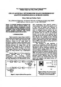
zero mathematical expectation and disperse 0,03 and impulse noise with density of the distribution 0,02. On the grounds of the results from processing these images with a Kalman filter and CNN neural network, a comparative analysis of the precision of the two approaches is done at filtration of the noised image. The comparison is done on the basis of two geometrical characteristics (features) of the target (plane): length of the fuselage axis and width (spread) of the wings of the plane. The approach at filtration to be chosen is the one in which the values of the two characteristics approximate at the most to those of the ‘etalon’ plane. A procedure is created in Matlab for estimating the length and the width of the plane, as well as for evaluating the precision of the two approaches. [7]. On figures 1, 2, 3 are presented respectively the ‘etalon’ image of an examined plane В 52, its image with background noise, eliminating the noise with a Kalman filter and CNN neural network, as well as moving to a black and white image from an image in a level of grey.
а)
b) Fig.1. Digital image of B52: a) output image; b) image with background noise.
3 Computer simulation Digital radio-holographic images of 10 types of airplanes, which can serve as ‘etalon’ standard models, are used.[ 1 ] They are chosen at random. These are: F16, An 124, McDowell, B52, Buccaneer, F117, Jaguar, Mig 29, Miraj 2000, Su 34..Reconstructed radio-holographic images of the same types of planes are examined, which have additive Gaussian noise with normal distribution at
а)
b)
Fig.2. Image subject to processing with Kalman filter: а) filtered image; b) black and white image of the target
7th WSEAS Int. Conf. on MATHEMATICAL METHODS and COMPUTATIONAL TECHNIQUES IN ELECTRICAL ENGINEERING, Sofia, 27-29/10/05 (pp31-36)
а)
b)
Fig.3. Image subject to processing via CNN neural network: а) filtered image; b) black and white image of the target.
Graphic User Interface (GUI), shown in fig.4, is created to achieve filtration of an image according to Kalman method.
Via the interface one can choose: ¾ the number of repetitions of the filtration; ¾ threshold of the grey – for producing a binary image; ¾ identification of a target in the image. Both the input and the filtered images are visualized. Candy software is used for achieving filtration via CNN neural network. This software product fulfils a lot of functions, part of which are connected with image filtration. Processing of an image is shown in fig. 6.
Fig.6. Filtration of a digital image with CNN neural network in Candy programme medium.
Opportunity is given for choosing the operation, the time of its accomplishment, the step of discretion, etc. Fig. 4. General view of GUI for filtration of a digital image according to Kalman method.
The interface gives the opportunity for downloading the image from a file via a dialogue window, shown in fig.5.
Fig.5. Dialogue window for choosing a file with an image.
4 Comparative analysis of the results of filtration with Kalman filter and CNN neural network After processing the images with Kalman and CNN neural network, their geometrical characteristics are calculated. A procedure in Matlab is used [7]. Their numerical values are shown in table 1. The length of the fuselage axis and the width of the wings, are the number of pixels, respectively between the head and the tail of the plane and the endmost points of the two wings. The absolute error could be used as a criterion for fidelity. It is as follows: δ x = xет − xизм (18) where x ет is the value of the parameter of the standard target; x изм - the value of the parameter of the target after using a certain filter.
7th WSEAS Int. Conf. on MATHEMATICAL METHODS and COMPUTATIONAL TECHNIQUES IN ELECTRICAL ENGINEERING, Sofia, 27-29/10/05 (pp31-36)
The fidelity of an approximation is better ∧
characterized by the relative error δ x (х) equal to the ratio of the absolute error to the calculated value:[6] ∧ δ δ x = x .100, % (19) xизм
3 4 5 6 7 8 9
MD B52 Bucan F117 Jaguar Mig29 Miraj 2000 Su34
10
5 Conclusion
32 98
47 89
29 90
68 56 49 50 78 42 49
58 67 35 37 44 37 30
66 54 47 48 75 39 47
57 64 33 35 41 32 26
87
61
86
60
84
55
Spread of wings
49 90
69 56 50 51 80 43 50
33 10 0 59 68 36 38 45 38 31
Length of fuselage axis
50 91
Spread of wings
Length of fuselage axis
F16 АN
Target after Kalman filter
Spread of wings
1 2
Target after processing with CNN NN
Length of fuselage axis
Standard target
Table 1. Geometrical characteristics of planes.
The values of the relative error for the examined types of planes, calculated according to (19) are shown in table 2. Type of plane
∧
δ x, Length of the fuselage axis Kalman CNN 6.38 2.04 1.12 1.11 4.55 1.47 3.7 0 6.38 2.04 6.25 2 6.67 2.56 10.25 2.38 6.66 2.04
∧
The value δ x =5 % is usually considered acceptable [4]. From the results one can see that the relative error, resulting from the different values of the characteristics at the use of CNN neural network, is less than 5%. When Kalman filter is used, it comes up to 10.25% for the length of the fuselage axis and up to 19.23 % for the spread of the wings.
% Width of wings
Kalman CNN 13.79 3.13 F16 11.11 2.04 АN 3.5 1.72 MD 6.25 1.49 B52 9.09 2.85 Bucan 8.57 2.7 F117 9.75 2.27 Jaguar 18.75 2.78 Mig29 19.23 3.33 Miraj 2000 3.57 1.16 10.9 1.67 Su34 Table 2. Values of the relative error for each type of planes
The processing of images is a n important stage in the process of identifying a target. On the grounds of the research done and described above we can summarize that the application of an intelligent approach at filtration of a radio-holographic image leads to better results in comparison with the classical approach. The use of CNN neural network guarantees a greater exactness at taking down the geometrical features of a target and hence more precise identification.
References: [1] http://spacecom.gvc.nasa.goviensconf [2] Guo, L Estimating time-varying parameters by the Kalman filter based algorithm: Stability and convergence, IEEE Transactions on Automatic Control, Vol.35, No.2, 1990, pp. 141-147. [3] Kragmann, U., Machine Intelligence as Applied to Future Autonomous Tactical Systems, RTO Symposium, Monterey, CA 20-22 April 1998. [4] Lazarov, A.. D., Minchev, Ch.M. Algorithm for ISAR Target Recognition and Neural Network Architecture Implementation, In proceedings of ISPC 2003, Dallas, Texas, USA, March 31-April 3, 2003. [5] Proc. IEEE Int. Workshop on Cellular Neural Networks and Their Applications (CNNA-92), 1992, Munich. [6] Gatev K., General theory of statistics, UNSS, Sofia, 1986. (in Bulgarian). [7] Popov, Z., Naumov V., Nedev A., Analysis and design of SAR and SAU with MAtlab, TU-Varna, 2001 (in Bulgarian).