Jan 4, 2008 - List of Figures. 1.1 Development costs for three SoC products . .... refers to it as VMX (Vector Multimedia eXtension), Apple as Velocity Engine.
Programming and compiling for embedded SIMD architectures
Anton Lokhmotov
University of Cambridge Computer Laboratory Robinson College
4 January 2008
The dissertation is submitted for the degree of Doctor of Philosophy
Declaration
This dissertation is the result of my own work and includes nothing which is the outcome of work done in collaboration except where specifically indicated in the text. I confirm that this dissertation, including tables and footnotes, but excluding appendices, bibliography and diagrams, does not exceed the regulation length of 60 000 words. Signed,
Anton Lokhmotov
2
Summary
This dissertation studies programming and compiling for embedded SIMD architectures, which deliver high-performance at low power consumption for many important application domains ranging from multimedia processing to scientific computing. We review the evolution of SIMD architectures from their inception in supercomputers in the 1960–1970s to recent embedded implementations, and the means for programming them efficiently: from using compiler-known functions in sequential languages to data-parallel languages to automatic parallelisation. We identify design choices of data-parallel programming languages and relate their efficiency and portability to the capabilities of target architectures. We propose a novel language construct that allows the programmer to express the independence of operations within a block of statements, which relieves the compiler from complex (and often intractable in practice) data dependence analysis and makes code more amenable to automatic parallelisation. We investigate (using bit-reversed data copy as an example problem) how vector shuffle instructions can be used optimally to improve program efficiency. Overall, the dissertation asserts that SIMD architectures will continue to play an important rˆole in the future, because of the efficiency they provide for data-parallel problems and the natural programming model.
3
Acknowledgements
It is impossible to acknowledge properly all the people who helped me to shape this dissertation, but I am profoundly indebted to Professor Alan Mycroft, my supervisor, for his incessant guidance, support and care, and for his recommendation for a summer internship at Broadcom that triggered this dissertation. I thank my industrial collaborators for providing research materials and helpful discussions: Sophie Wilson, John Redford and Neil Johnson from Broadcom, Cambridge; Marcel Beemster, Joseph van Vlijmen, Liam Fitzpatrick and Hans van Someren from ACE Associated Compiler Experts, Amsterdam; Benedict Gaster from ClearSpeed Technology, Bristol; Alastair Donaldson and Andrew Richards from Codeplay Software, Edinburgh; Alastair Reid from ARM, Cambridge. I also thank Viktor Vafeiadis, my office-mate for three years, who explained to me many interesting concepts and was able to understand my research ideas (although I could hardly understand his). I gratefully acknowledge the financial support by a TNK-BP Cambridge Kapitza Scholarship and by an Overseas Research Students Award, which allowed me to study at Cambridge. But I would have never aspired to this, if it were not for my mentors and colleagues from Moscow Chemical Lyceum, Moscow Institute of Physics and Technology, and Institute for Systems Programming RAS, to whom I express my deepest gratitude. I also thank the University of Cambridge and its clubs and societies, for providing so many opportunities for active life and personal development, in particular, CU Hillwalking Club, Robinson College Boat Club and, most importantly, CU Russian Society, engagement with which not only has made me less homesick but also this dissertation thinner. Last, but not least, I would like to thank my family and friends (this list is unexcusably brief): mum Laura (simply for always being there), granny Masha (the first PhD in my family!), Nadya (for her love and understanding), and my dear friends (for being so wonderful)!
4
Author Publications
Parts of this research have been published in the following papers: [1] Anton Lokhmotov and Alan Mycroft. Optimal bit-reversal using vector permutations (brief announcement). In Proceedings the 19th Annual ACM Symposium on Parallelism in Algorithms and Architectures (SPAA), pages 198–199, New York, NY, USA, 2007. ACM Press. [2] Anton Lokhmotov and Alan Mycroft. Nested loop vectorisation. In Proceedings of the 2nd International Summer School on Advanced Computer Architecture and Compilation for Embedded Systems (ACACES), pages 87–91, Ghent, Belgium. Academia Press, 2006. [3] Anton Lokhmotov, Benedict R. Gaster, Alan Mycroft, Neil Hickey and David Stuttard. Revisiting SIMD programming. In Proceedings of the 20th Workshop on Languages and Compilers for Parallel Computing (LCPC). To appear in Lecture Notes in Computer Science. Springer, 2008. [4] Anton Lokhmotov, Alan Mycroft and Andrew Richards. Delayed side-effects ease multicore programming. In Proceedings of the 13th European Conference on Parallel and Distributed Computing (Euro-Par), volume 4641 of Lecture Notes in Computer Science, pages 629–638. Springer, 2007. [5] Alastair Donaldson, Colin Riley, Anton Lokhmotov and Andrew Cook. Auto-parallelisation of Sieve C++ programs. In Proceedings of the Workshop on Highly Parallel Processing on a Chip (HPPC), volume 4854 of Lecture Notes in Computer Science, pages 18–27. Springer, 2008. [6] Anton Lokhmotov, Alastair Donaldson, Alan Mycroft and Colin Riley. Strict and relaxed sieving for multi-core programming. In Proceedings of the Workshop on Programmability Issues for Multi-Core Computers (MULTIPROG). 2008. Chapter 3 includes an account of the Cn language designed by ClearSpeed and reported in [3]. The author gives the design rationale of the language, and compares Cn with other languages for SIMD architectures designed over the past 40 years. The Cn compiler improvement data is courtesy of ClearSpeed. Chapter 4 describes the concept of sieving originally introduced in Codeplay’s C++ extension and refined in [4] ([5] describes other features of that extension, which Chapter 4 mentions only briefly). The author gives a rather different formulation, called relaxed sieving, in [6]. The experimental data is courtesy of Codeplay. 5
Contents
Glossary
13
1
Introduction
15
1.1
Embedded systems and the rˆole of software . . . . . . . . . . . . . . . . . . .
15
1.2
Embedded high-performance computing . . . . . . . . . . . . . . . . . . . . .
17
1.3
Supercomputing meets embedded computing . . . . . . . . . . . . . . . . . .
17
1.4
Vector processing in general-purpose computing . . . . . . . . . . . . . . . . .
18
1.5
Dissertation outline . . . . . . . . . . . . . . . . . . . . . . . . . . . . . . . .
18
2
SIMD architectures: past, present. . . and future?
20
2.1
Parallel SIMD supercomputers . . . . . . . . . . . . . . . . . . . . . . . . . .
21
2.1.1
Solomon . . . . . . . . . . . . . . . . . . . . . . . . . . . . . . . . .
21
2.1.2
Illiac IV . . . . . . . . . . . . . . . . . . . . . . . . . . . . . . . . . .
22
2.1.3
Connection Machine . . . . . . . . . . . . . . . . . . . . . . . . . . .
22
2.1.4
Other parallel SIMD supercomputers . . . . . . . . . . . . . . . . . .
23
Pipelined SIMD supercomputers . . . . . . . . . . . . . . . . . . . . . . . . .
23
2.2.1
Cray-1 . . . . . . . . . . . . . . . . . . . . . . . . . . . . . . . . . .
24
2.2.2
Other pipelined SIMD supercomputers . . . . . . . . . . . . . . . . .
24
Embedded SIMD processors . . . . . . . . . . . . . . . . . . . . . . . . . . .
25
2.3.1
ClearSpeed CSX . . . . . . . . . . . . . . . . . . . . . . . . . . . . .
25
2.3.2
NEC IMAP . . . . . . . . . . . . . . . . . . . . . . . . . . . . . . . .
26
2.3.3
Broadcom FirePath . . . . . . . . . . . . . . . . . . . . . . . . . . . .
27
2.3.4
Sony/Toshiba/IBM Cell SPU . . . . . . . . . . . . . . . . . . . . . . .
28
2.4
Modern processors vs. traditional supercomputers . . . . . . . . . . . . . . . .
28
2.5
Summary . . . . . . . . . . . . . . . . . . . . . . . . . . . . . . . . . . . . .
29
2.2
2.3
6
3
Programming vector architectures
30
3.1
Low-level programming means . . . . . . . . . . . . . . . . . . . . . . . . . .
31
3.1.1
Example of programming in assembly . . . . . . . . . . . . . . . . . .
31
3.1.2
Soothing the pain of assembly programming . . . . . . . . . . . . . .
37
3.1.3
Summary . . . . . . . . . . . . . . . . . . . . . . . . . . . . . . . . .
41
Cn programming language . . . . . . . . . . . . . . . . . . . . . . . . . . . .
41
3.2.1
Cn design goals and choices . . . . . . . . . . . . . . . . . . . . . . .
41
3.2.2
Cn outline . . . . . . . . . . . . . . . . . . . . . . . . . . . . . . . .
43
3.2.3
Cn design rationale . . . . . . . . . . . . . . . . . . . . . . . . . . . .
47
3.2.4
Cn as intermediate language . . . . . . . . . . . . . . . . . . . . . . .
49
3.2.5
Cn compiler implementation . . . . . . . . . . . . . . . . . . . . . . .
51
3.2.6
Summary . . . . . . . . . . . . . . . . . . . . . . . . . . . . . . . . .
53
Summary and future work . . . . . . . . . . . . . . . . . . . . . . . . . . . .
53
3.3.1
53
3.2
3.3
4
Machine-independent vector processing . . . . . . . . . . . . . . . . .
Automatic parallelisation
55
4.1
Dependence analysis . . . . . . . . . . . . . . . . . . . . . . . . . . . . . . .
56
4.1.1
Data dependence and parallelisation . . . . . . . . . . . . . . . . . . .
56
4.1.2
Aliasing complicates dependence analysis . . . . . . . . . . . . . . . .
64
Delayed side-effects ease automatic parallelisation . . . . . . . . . . . . . . .
65
4.2.1
Introduction . . . . . . . . . . . . . . . . . . . . . . . . . . . . . . . .
65
4.2.2
Explaining sieve semantics . . . . . . . . . . . . . . . . . . . . . . . .
66
4.2.3
Mary Hope and the Delayed Side-Effects . . . . . . . . . . . . . . . .
71
4.2.4
Importance of sieving . . . . . . . . . . . . . . . . . . . . . . . . . .
73
4.2.5
Strict and relaxed sieving . . . . . . . . . . . . . . . . . . . . . . . . .
75
4.2.6
Why sieving? . . . . . . . . . . . . . . . . . . . . . . . . . . . . . . .
76
Experimental evaluation . . . . . . . . . . . . . . . . . . . . . . . . . . . . .
78
4.3.1
Homogeneous x86 multi-core system . . . . . . . . . . . . . . . . . .
78
4.3.2
Heterogeneous Cell BE processor . . . . . . . . . . . . . . . . . . . .
81
Related work . . . . . . . . . . . . . . . . . . . . . . . . . . . . . . . . . . .
81
4.4.1
Language extensions to enable automatic parallelisation . . . . . . . .
82
4.4.2
Programming explicitly managed memory hierarchies . . . . . . . . .
83
Summary and future work . . . . . . . . . . . . . . . . . . . . . . . . . . . .
84
4.5.1
84
4.2
4.3
4.4
4.5
Self-prefetching data structures . . . . . . . . . . . . . . . . . . . . .
7
5
Automatic vectorisation: a survey
86
5.1
Classical vectorisation . . . . . . . . . . . . . . . . . . . . . . . . . . . . . .
87
5.2
Straight-line code vectorisation . . . . . . . . . . . . . . . . . . . . . . . . . .
88
5.2.1
Vectorisation by loop unrolling . . . . . . . . . . . . . . . . . . . . . .
88
5.2.2
Vectorisation of straight-line numerical code . . . . . . . . . . . . . .
89
5.2.3
Vectorisation by instruction selection . . . . . . . . . . . . . . . . . .
90
5.3
Alignment constraints . . . . . . . . . . . . . . . . . . . . . . . . . . . . . . .
90
5.4
Idiom recognition . . . . . . . . . . . . . . . . . . . . . . . . . . . . . . . . .
92
5.4.1
Rigid pattern matching . . . . . . . . . . . . . . . . . . . . . . . . . .
92
5.4.2
Augmenting classical vectorisation with pattern matching . . . . . . .
92
Miscellaneous . . . . . . . . . . . . . . . . . . . . . . . . . . . . . . . . . . .
93
5.5.1
Vectorisation of control flow . . . . . . . . . . . . . . . . . . . . . . .
93
5.5.2
Vector replacement . . . . . . . . . . . . . . . . . . . . . . . . . . . .
93
5.5.3
Energy-aware vectorisation . . . . . . . . . . . . . . . . . . . . . . . .
93
5.5.4
Symbolic vectorisation . . . . . . . . . . . . . . . . . . . . . . . . . .
94
Retargetable vectorisation . . . . . . . . . . . . . . . . . . . . . . . . . . . . .
94
5.6.1
GNU GCC . . . . . . . . . . . . . . . . . . . . . . . . . . . . . . . .
94
5.6.2
IBM XL . . . . . . . . . . . . . . . . . . . . . . . . . . . . . . . . . .
95
5.6.3
COINS . . . . . . . . . . . . . . . . . . . . . . . . . . . . . . . . . .
95
5.6.4
ACE CoSy . . . . . . . . . . . . . . . . . . . . . . . . . . . . . . . .
95
5.5
5.6
6
Vector shuffles
96
6.1
Vector shuffle instructions . . . . . . . . . . . . . . . . . . . . . . . . . . . .
96
6.2
Bit-reversal using vector shuffles: motivation . . . . . . . . . . . . . . . . . .
98
6.2.1
Bit-reversal . . . . . . . . . . . . . . . . . . . . . . . . . . . . . . . .
99
6.2.2
Motivating example . . . . . . . . . . . . . . . . . . . . . . . . . . . 100
6.3
Bit-reversal using vector shuffles . . . . . . . . . . . . . . . . . . . . . . . . . 102 6.3.1
Assumptions and notation . . . . . . . . . . . . . . . . . . . . . . . . 102
6.3.2
Placing elements into vectors . . . . . . . . . . . . . . . . . . . . . . . 103
6.3.3
A basic property of the index reversal . . . . . . . . . . . . . . . . . . 103
6.3.4
Identifying classes of vectors . . . . . . . . . . . . . . . . . . . . . . . 104
6.3.5
Paralellism corollary . . . . . . . . . . . . . . . . . . . . . . . . . . . 105
6.3.6
Using interleaving operations . . . . . . . . . . . . . . . . . . . . . . 106
6.3.7
Analysis
6.3.8
Basic algorithm . . . . . . . . . . . . . . . . . . . . . . . . . . . . . . 109
. . . . . . . . . . . . . . . . . . . . . . . . . . . . . . . . . 106
8
6.3.9
Cache-optimal extension . . . . . . . . . . . . . . . . . . . . . . . . . 109
6.3.10 Experimental results . . . . . . . . . . . . . . . . . . . . . . . . . . . 110 6.4
6.5
7
Related work . . . . . . . . . . . . . . . . . . . . . . . . . . . . . . . . . . . 116 6.4.1
Generating shuffle instructions . . . . . . . . . . . . . . . . . . . . . . 116
6.4.2
Minimising shuffle instructions . . . . . . . . . . . . . . . . . . . . . 118
Future work . . . . . . . . . . . . . . . . . . . . . . . . . . . . . . . . . . . . 118 6.5.1
Discovering vector shuffles . . . . . . . . . . . . . . . . . . . . . . . . 119
6.5.2
Decomposing vector shuffles . . . . . . . . . . . . . . . . . . . . . . . 120
6.5.3
Designing application-specific instructions . . . . . . . . . . . . . . . 120
6.5.4
Possible link to interconnection networks . . . . . . . . . . . . . . . . 121
6.5.5
Summary . . . . . . . . . . . . . . . . . . . . . . . . . . . . . . . . . 122
Conclusion and future work
123
7.1
Conclusion . . . . . . . . . . . . . . . . . . . . . . . . . . . . . . . . . . . . 123
7.2
Future work . . . . . . . . . . . . . . . . . . . . . . . . . . . . . . . . . . . . 124 7.2.1
Background . . . . . . . . . . . . . . . . . . . . . . . . . . . . . . . . 124
7.2.2
Programme and methodology . . . . . . . . . . . . . . . . . . . . . . 126
7.2.3
Summary . . . . . . . . . . . . . . . . . . . . . . . . . . . . . . . . . 129
Bibliography
130
9
List of Figures
1.1
Development costs for three SoC products . . . . . . . . . . . . . . . . . . . .
16
3.1
Cn compiler improvement from version 2.51 to version 3.0 . . . . . . . . . . .
52
4.1
C implementation of computing the Mandelbrot fractal . . . . . . . . . . . . .
58
4.2
Cn implementation of computing the Mandelbrot fractal . . . . . . . . . . . .
62
4.3
Illustrative memory access schedules . . . . . . . . . . . . . . . . . . . . . . .
66
4.4
Implementations of a one-dimensional mean filter in C, C99 and Sieve C++ . .
72
4.5
Speedup of Sieve C++ code w.r.t. original C++ code on x86 . . . . . . . . . . .
80
4.6
Memory overhead of sieving on x86 . . . . . . . . . . . . . . . . . . . . . . .
81
4.7
Speedup of Sieve C++ code w.r.t. single SPE on Cell BE . . . . . . . . . . . .
82
6.1
Example vector shuffle operations . . . . . . . . . . . . . . . . . . . . . . . .
97
6.2
The 16-point bit-reversal using vector shuffles . . . . . . . . . . . . . . . . . .
98
6.3
The 32-point bit-reversal using P2→2 interleaving shuffles . . . . . . . . . . . . 102
6.4
Array index partitioning . . . . . . . . . . . . . . . . . . . . . . . . . . . . . 103
6.5
Bit-reversal on SSE2 . . . . . . . . . . . . . . . . . . . . . . . . . . . . . . . 111
6.6
Bit-reversal on AltiVec . . . . . . . . . . . . . . . . . . . . . . . . . . . . . . 112
6.7
Bit-reversal on Cell . . . . . . . . . . . . . . . . . . . . . . . . . . . . . . . . 113
6.8
Selecting orderings for vector groups . . . . . . . . . . . . . . . . . . . . . . . 117
6.9
The 4 × 4 matrix trasposition using interleaving shuffles . . . . . . . . . . . . 119
6.10 Rearrangeable shuffle-exchange network with N = 16 inputs/outputs . . . . . 121
10
List of Tables
4.1
Memory-based dependences in the Mandelbrot code . . . . . . . . . . . . . .
59
4.2
Codeplay’s Sieve C++ benchmarks . . . . . . . . . . . . . . . . . . . . . . . .
79
6.1
Experimental systems for bit-reversal algorithms . . . . . . . . . . . . . . . . 114
7.1
Communication vs. computation costs in 130nm and 45nm processes . . . . . . 125
11
List of Listings
3.1
FIR filter implementation in C99 . . . . . . . . . . . . . . . . . . . . . . . . .
32
3.2
FIR filter inner loop. Compiler-generated Cortex-R4 code . . . . . . . . . . . .
32
3.3
FIR filter inner loop. Improved scalar Cortex-R4 code . . . . . . . . . . . . . .
33
3.4
FIR filter inner loop. Basic vector Cortex-R4 code . . . . . . . . . . . . . . . .
33
3.5
FIR filter inner loop. Software-pipelined vector Cortex-R4 code . . . . . . . .
34
3.6
FIR filter vectorisation via inner loop unrolling . . . . . . . . . . . . . . . . .
35
3.7
FIR filter vectorisation via outer loop unrolling . . . . . . . . . . . . . . . . .
36
3.8
FIR filter inner loop. Software-pipelined vector FirePath code . . . . . . . . .
37
3.9
Bit-reversal kernel for 32-bit data on AltiVec. . . . . . . . . . . . . . . . . . .
38
3.10 Bit-reversal kernel for 32-bit data on SSE2. . . . . . . . . . . . . . . . . . . .
39
3.11 Bit-reversal kernel for 32-bit data on Cell SPU. . . . . . . . . . . . . . . . . .
40
3.12 Example code using CSX intrinsics . . . . . . . . . . . . . . . . . . . . . . .
52
12
Glossary
3G The third generation of mobile phone standards. ADSL Asymmetric DSL A version of DSL that reserves more bandwidth for downstream transfers (to the user) than for upstream transfers (from the user). Standard ADSL provides peak rates of 8Mbit/s downstream and 1Mbit/s upstream. ADSL2 extends the peak rates to 12Mbit/s and 3.5Mbit/s, while ADSL2+ pushes the peak upstream rate to 24Mbits/s. AltiVec PowerPC instruction set multimedia extension. AltiVec is Motorola’s trade name. IBM refers to it as VMX (Vector Multimedia eXtension), Apple as Velocity Engine. ASIC Application-Specific Integrated Circuit An IC implementing a specific function. BLAS Basic Linear Algebra Subprograms Standardised application programming interfaces for subroutines to perform basic linear algebra operations such as vector and matrix multiplication. CO Central Office Generally refers to the communication service provider’s premises or equipment such as DSL modems. DGEMM Double precision floating point matrix-matrix multiplication. DLP Data-Level Parallelism DSL Digital Subscriber Line A family of technologies that provide digital data transmission over the wires of a local telephone network. FLOPS Floating-point Operations Per Second A measure of a computer’s performance. Usually refers to either single or double floating point precision. The standard SI prefixes apply, e.g. GigaFLOPS = 109 FLOPS, TeraFLOPS = 1012 FLOPS. FPGA Field-Programmable Gate Array An IC containing logic components and interconnects that can be programmed (and often re-programmed) to implement a specific function. Usually slower and draw more power than non-programmable ICs.
13
HPC High-Performance Computing The use of computers to support scientists, engineers and other analysts in doing numerically or data intensive work. This includes computing systems from workstations and servers to supercomputers. HSDPA High-Speed Downlink Packet Access A 3G mobile telephony protocol with the peak downlink rate of 14.4 Mbit/s. HSPA High-Speed Packet Access A family of 3G mobile telephony protocols including HSDPA and HSUPA. HSUPA High-Speed Uplink Packet Access A 3G mobile telephony protocol with the peak uplink rate of 5.76 Mbit/s. IC Integrated Circuit A miniaturised electronic circuit manufactured in the surface of a thin substrate of semiconductor material. ILP Instruction-Level Parallelism A measure of how many of the instructions in a sequential program can be executed in parallel. LINPACK A software library for performing numerical linear algebra. Makes use of BLAS. The LINPACK benchmark measures how fast a computer solves a dense n × n system of linear equations Ax = b, based on Gaussian elimination with partial pivoting, with 2/3n3 + n2 floating point operations. The problem is very regular and the performance numbers give a good correction of peak performance. MMX MultiMedia eXtension Intel instruction set multimedia extension (1996). Operates on packed data in 64-bit registers (8 registers; aliased to FPU registers). MPEG-2 Moving Pictures Expert Group A standard describing lossy video and audio compression methods for broadcast-quality television. SIMD Single Instruction Multiple Data SoC System-on-Chip An IC impementing a number of components (such as processor cores, memory, peripherals and interfaces) on a single die. SSE Streaming SIMD Extension Intel instruction set multimedia extension. Versions: SSE (1999), SSE2 (2001), SSE3 (2004), SSSE3 (2005), SSE4 (2006). TLP Thread-Level Parallelism TOP500 A list of the 500 most powerful publicly-known computer systems in the world. First published in 1993; is updated twice a year. The rankings are based on HPL, a portable implementation of the High-Performance LINPACK benchmark for distributed-memory computers. The system must be general-purpose, that is it must be able to solve a range of scientific problems (any system specifically designed to execute the LINPACK benchmark is disqualified). VDSL Very High Speed DSL A version of DSL with peak rates of 26Mbit/s for symmetric access or 52Mbit/s downstream and 12Mbit/s upstream for asymmetric access (see ADSL). VSDL2 extends the aggregate peak rate to 200Mbit/s. VIS Visual Instruction Set SPARC instruction set multimedia extension.
14
CHAPTER 1
Introduction
E X PRAETERITO PRAESENS PRVDENTER AGIT NI FVTVR ACTIONE DETVRPET. [Learning] from the past, the man of the present acts prudently, so as not to imperil the future. —Inscribed on “An Allegory of Prudence” by Titian (1485–1576), National Gallery, London.
1.1
Embedded systems and the rˆole of software
Embedded systems are special-purpose electronic devices permeating the modern world. Examples range from smart cards and music players to digital cameras and TV sets. Embedded systems are actually “computers in disguise”, as they rely on a combination of hardware and software components.1 As the world is becoming increasingly digital, embedded systems represent the fastest growing portion of the computing market [50]. While business opportunities abound, the competition is often fierce, and short time-to-market is critical to success. Typical customer requirements include low cost and low power consumption (especially for portable electronics running on batteries). Designing an Application-Specific Integrated Circuit (ASIC) is attractive because a waste of transistors in general-purpose designs translates into a waste of power (and money). Fixed function and large costs of prototyping and debugging, however, increase the business risk of delivering an uncompetitive product. Field-Programmable Gate Array (FPGA) designs offer flexibility but at the expense of distressing silicon inefficiency (meaning slower speed and higher power consumption). 1
The presence of computers in consumer electronics is not immediately obvious to people used to think that a computer is a colourful monitor connected to a noisy box. But even computer scientists need an effort to acknowledge that the cyborg in James Cameron’s Terminator is an embedded system.
15
3G HSDPA (2005)
Chip design Chip verification System and software
DSL CO (2001)
MPEG2 STB (1997)
0
50
100
150
200
250
300
350
400
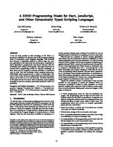
Figure 1.1: Development costs (approximate man years; one man year is estimated as $200K) for three SoC products: ST Chameleon CM10 (1997), Broadcom Santorini (2001), and Icera Livanto (2005). The costs include chip design, its functional verification, and systems and software engineering necessary to sell the product. Non-recurring mask manufacturing costs ($1–2M) are not shown. Instead, the market is turning to software-programmable designs, which allow post-manufacturing customisation and upgrades, including improved algorithms and bug fixes. Figure 1.1 shows estimated development costs for three software-based System-on-Chip (SoC) products [65]: • ST Chameleon CM10 (1997, 350nm): MPEG-2 set-top box based on the Chameleon processor; • Broadcom Santorini (2001, 130nm): Digital Subscriber Line (DSL) Central Office (CO) modem based on the FirePath processor; • Icera Livanto (2005, 90nm): 3G High-Speed Downlink Packet Access (HSDPA) modem based on the DXP processor. ST Chameleon CM10 was 25% larger and drew more power than the best fixed-function competitor [65]. Broadcom Santorini (BCM6410) had smaller area and consumed less power than many fixedfunction competitors and thus became the market leader (with one million chips shipped by May 2003). Moreover, the software-based design provided the agility to track emerging standards, which allowed the company to release later BCM6411 supporting ADSL2+ and BCM6510 supporting both ADSL2+ and VDSL2 standards [137]. Icera Livanto (ICE8020) embodies an even more radical design approach. While Chameleon and Santorini included application-specific instructions (20–25% of the full instruction set [65]), Livanto is claimed to have no hardware acceleration. Thus, the current products supporting HSDPA are upgradeable in software to support HSUPA on the same (small area and low power) silicon. Figure 1.1 shows that chip design and verification (the first two segments of the bars) take a diminishing fraction of the product development costs. Supporting new requirements in software would extend the last segment even further. Thus, this thesis adopts a biased, software-centric view. 16
1.2
Embedded high-performance computing
Consumer markets are driven by the increasing appetite of users for better and cheaper devices. For example, fifteen years ago mobile phone users could be excited by the ability to make a voice call from everywhere; today they demand mobile video conferencing of the highest quality. Better features often require real-time execution. For example, in an image recognition application detecting potential vehicle collisions, the processing must be done within milliseconds to ensure the safety of passengers. Thus, a system design is only viable if it allows application performance requirements to be meet. Most processors use pipelining to overlap the execution of instructions and thus improve performance [50]. Ideally (in the absence of pipeline stalls), an instruction is issued (and another completed) every clock cycle, so the performance grows linearly with the clock frequency.2 Unfortunately, the power consumption of a chip is proportional, in practice, to the cube of its operating frequency [21], so raising the frequency until the performance requirements are met is not power efficient. Superscalar processors can issue multiple instructions per cycle. But given that InstructionLevel Parallelism (ILP) has its limits [132], additional issue and execution logic provides diminishing performance gains, while increases power consumption [50]. Similarly, out-of-order execution decreases performance per unit power. Despite this apparent power trap, computer architects have found a way out. If increasing the number of instructions per cycle is difficult, why not increase the amount of work per instruction? Indeed, such increase is possible if a single instruction performs multiple operations. This idea (dating back to the 1960s) is known as Single Instruction Multiple Data (SIMD), or vector, processing. Combined with other techniques, it clears the route to low cost and power efficient high-performance computing. For example, the Icera DXP processor can achieve over a hundred of arithmetic operations per cycle on 16-bit data packed into 64-bit vector registers [65].
1.3
Supercomputing meets embedded computing
Science and engineering rely heavily on “supercomputers” capable of executing many trillions floating point operations per second (FLOPS) to process vast amounts of data and perform accurate simulations. While assembling clusters of commodity servers is a cost-effective way to achieve high performance, the electricity bills for powering and cooling of a typical server may exceed the cost of hardware over its useful lifetime of about three years. Thus, the procurement plans for large clusters now entangle a power budget with the hardware budget [49]. This casts doubt on the traditional way to build supercomputers by using the fastest (and most power-hungry) processor chips as the building blocks. As much as the embedded systems industry has learnt from the past how to achieve high performance, High-Performance Computing (HPC) is learning today from embedded computing how to achieve higher power efficiency. 2
Of course, this is a gross simplification, since higher frequency designs need deeper pipelines which are more susceptible to stalls and incur additional implementation overheads.
17
The IBM BlueGene/L system at Lawrence Livermore National Laboratory (USA) [69] has headed TOP500 (the list of the 500 fastest supercomputers in the world ranked by the number of FLOPS achieved on the LINPACK benchmark) since November 2004. BlueGene/L building blocks are embedded dual-core PowerPC 440 processors, with the peak performance of 2.8 GFLOPS per core running at 700 MHz. The LLNL system has 131,072 (217 ) cores and delivers 280.6 GFLOPS on the LINPACK, while consumes 1.6MW of power (which equates to 175 MFLOPS/W).3 In comparison, the Sun TSUBAME cluster installed in 2006 at the Tokyo Institute of Technology [91] with 10,368 AMD Opteron cores achieved 38.18 TFLOPS at 800KW (48 MFLOPS/W). However, with a later upgrade of 360 ClearSpeed Advance boards [127], the cluster delivered 47.38 TFLOPS at 810KW (58 MFLOPS/W). That is, the boards increased the cluster’s overall performance by 24%, while adding only 1% to the overall power consumption. Each ClearSpeed board has two CSX600 processors [27] for intensive double-precision floatingpoint computations, each providing 33 GFLOPS of sustained matrix multiply (DGEMM) performance, while dissipating an average of 10 watts (3.3 GFLOPS/W). This exceeds even the theoretical 230 MFLOPS/W of BlueGene/L. The CSX600 is so efficient because it is an array of 96 processing elements operating in lock-step according to the same SIMD paradigm that is used in the aforementioned DSP architectures. More efficient chips do exist. For example, the RIKEN MDGRAPE-3 chip for molecular dynamics simulations [24] running at 250MHz delivers 165 GFLOPS, while dissipates only 16 watts (10.3 GFLOPS/W). However, it can only perform force calculations,4 while the CSX600 is fully programmable.
1.4
Vector processing in general-purpose computing
General-purpose computing has also benefited from the SIMD paradigm. In the 1990s, the growing importance of multimedia workloads has resulted in the introduction of multimedia extensions to many general-purpose architectures. Examples include Intel MultiMedia eXtension (MMX)/Streaming SIMD Extension (SSE) [15], PowerPC AltiVec [31], and SPARC Visual Instruction Set (VIS) [128]. The current trend is to extend vector processing capabilities by adding more instructions and increasing the vector width (e.g. to 256–512 bits from today’s de facto standard of 128 bits).
1.5
Dissertation outline
This dissertation studies programming and compiling for SIMD architectures (either used in special-purpose processors or incorporated into general-purpose processors). 3
The IBM BlueGene/P is the next generation of BlueGene architecture based a quad-core PowerPC 450 processors, with a peak performance of 3.4 GFLOPS per core running at 850 MHz. BlueGene/P is designed to scale up to 1,048,576 (220 ) cores delivering over 3 PFLOPS on the LINPACK at estimated 260 MFLOPS/W. 4 For this reason, while the system including 5120 such chips is the first computer with the theoretical performance of 1 PFLOPS, it is not competitive on the LINPACK.
18
Chapter 2 Reviews the evolution of SIMD architectures from their inception in supercomputers (Illiac IV, Connection Machine, Cray-1) to recent embedded implementations (ClearSpeed CSX, Broadcom FirePath, Sony/Toshiba/IBM Cell SPU). Chapter 3 Identifies choices of programming means (from assembly and compiler-known functions to data-parallel languages) and relates their efficiency and portability to the capabilities of target architectures. Chapter 4 Proposes a novel language construct that allows the programmer to express the independence of operations within a block of statements, which relieves the compiler from complex (and often intractable in practice) data dependence analysis and makes code more amenable to automatic parallelisation. Chapter 5 Surveys automatic vectorisation techniques for short vector architectures and discusses challenges of supporting vectorisation in retargetable compilers. Chapter 6 Investigates (using bit-reversed data copy as an example problem) how vector shuffle instructions can be used optimally to improve program efficiency. Chapter 7
Concludes with an outline of future work.
19
CHAPTER 2
SIMD architectures: past, present. . . and future?
There are two extremes in machine design. At one extreme we have a completely parallel machine, in which all opportunities to increase the speed by parallel operation have been exploited. At the other extreme is the completely serial machine, in which all methods of reducing equipment by serial operation have been incorporated. There are of course many possible intermediate variations which are to some extent serial and to some extent parallel. —John William Mauchly (1907–1980) Moore School Lectures on Theory and Techniques for Design of Electronic Digital Computers (1946)
I’m certainly not inventing vector processors. There are three kinds that I know of existing today. They are represented by the ILLIAC IV, the (CDC) STAR processor, and the TI (ASC) processor. Those three were all pioneering processors. . . One of the problems of being a pioneer is you always make mistakes and I never, never want to be a pioneer. It’s always best to come second when you can look at the mistakes the pioneers made. —Seymour Cray (1925–1996) Public lecture at Lawrence Livermore Laboratory on the introduction of the Cray-1 (1976)
Even early computers were designed to overlap computation with input/output communication [136]. Later computers introduced pipelining which overlaps execution of successive instructions and issuing multiple instructions in one clock cycle. While these developments were in accord with John Mauchly’s vision, in which adding more equipment increased parallel operation (see the epigraph), it was not until the 1960s when parallel computers in the modern sense appeared. 20
Typical scientific programs perform the same (or almost the same) sequence of operations on different elements of a large data set.1 In this setting, the traditional computer operation, in which the processing unit fetches instructions from memory, decodes and executes them, is inefficient. The Single Instruction Multiple Data (SIMD) operation executes the same instruction over all elements of a data set and thus amortises the instruction fetching and decoding overhead over the whole set. Two principally different embodiments of the SIMD paradigm are parallel and pipelined computers. In parallel SIMD (or array) computers, data elements are distributed across multiple memories coupled to identical processing units. In pipelined SIMD (or vector) computers, data elements are stored in shared memory and are brought into pipelined functional units for processing. This chapter overviews pioneering parallel (§2.1) and pipelined (§2.2) SIMD supercomputers, with a focus on their principal organisation, but not on their implementation technology,2 and presents several embedded SIMD architectures (§2.3).
2.1
Parallel SIMD supercomputers
2.1.1 Solomon The Solomon computer [46], designed by the Westinghouse Electric Corporation in 1962–1964 under a contract from the US Air Force, is the first prototype SIMD system (even before Flynn coined the term “SIMD” in [38]). The Solomon has three principal components: the control unit (CU), the network of processing elements (PEs) and the I/O unit. The basic PE network consists of 32 × 32 PEs organised in 32 × 8 modules. The control unit steps through a single instruction stream and recognises instructions of four types: CU arithmetic instructions, CU control flow instructions (jumps), I/O instructions, and PE instructions. The CU executes both types of CU instructions. The I/O unit controls the I/O data channels. The PE sequencer receives PE instructions from the CU, decodes them and sends control signals to the PE network. Each PE either executes or ignores a given instruction (a PE is said to be enabled or disabled, respectively). Each PE can be in one of four mode states, and also controlled geometrically, i.e. on the basis of its location in a particular row or column. Each PE instruction can specify any combination of the four mode states and whether to follow or to ignore the geometric control. Thus, a PE executes an instruction if both mode and geometric control specifications are met. Mode states can be stored into and loaded from PE memory. Each PE is connected to its four nearest neighbours in the network, which is basically arranged as a two-dimensional grid. The edge elements in the network can be configured (by a special instruction) to form a plane, a horizontal or vertical cylinder, a horizontal or vertical circle, or a torus. 1
“If a program manipulates a large amount of data, it does so in a small number of ways” [95]. Obviously, the early computers were huge, as even simple devices required large hardware blocks. Technology did not always match the aspirations of designers: desired components sometimes had to be replaced with slower but more readily available ones (e.g. this caused cost escalation and schedule delays for the Illiac IV [117]). 2
21
Each PE has two bit-addressed memory banks, or frames, of 4096 bits per frame (expandable up to 16,384 bits). Instructions have 72-bit encoding, allowing for two operands (one of which is replaced by the result). The operands are transferred to the arithmetic logic operating on words of variable length (between 1 and 128 bits). The operands come either from the frames (of the PE or of its neighbours via the routing logic) or from the CU broadcast register (allowing data in common between PEs to be stored in the CU memory and supplied via the broadcast register when needed).
2.1.2 Illiac IV Daniel Slotnick, one of the principle investigators on the Solomon project, moved to the University of Illinois and started the Illiac IV project under a DARPA contract after the Solomon project money had run out. The Burroughs Corporation was the principal partner, providing the B6500 general-purpose computer (a user ‘front-end’ for preparing programs and managing I/O) and disk subsystem. The original design [11] provides for 256 PEs arranged in four arrays, each containing 64 PEs and a CU. The four arrays can be configured to operate as a single 256 PE system, two 128 PE systems, or four 64 PE systems. In multi-array configurations (1 × 256 and 2 × 128 PEs), the CUs step through a single instruction stream independently, synchronising only when data or control signals need to cross array boundaries. The instruction buffer holds a maximum of 128 instructions (sufficient to hold the inner loop of many programs), which get prefetched in blocks of 16 instructions. CU and PE instruction executions may overlap, so scheduling is important. The CU has access to the entire array memory, while each PE can only reference its local memory of 2048 64-bit words. PE addresses are formed by summing three components: a fixed address in the instruction, a CU index value from one of the CU accumulators, and a local PE index value. Each PE is connected to its four nearest neighbours in the 8 × 8 array (i.e. with distances ±1 and ±8) and to the disk subsystem. Processor partitioning allows to make efficient use of the hardware when the full 64-bit precision is not required. Each processor can be partitioned into either two 32-bit or eight 8-bit subprocessors. Each 32-bit subprocessor has a separate enable bit; 8-bit subprocessors do not. In both cases, the subprocessors share a common index register. (This same idea reemerged in commodity microprocessors some 30 years later under the name of multimedia extensions.) The Illiac IV was not completed until 1972. By that time, the original $8 million estimated from the first design in 1966 had risen to $31 million (although only one array of four was delivered). Even worse, the machine was failing continually, and efforts to improve its reliability lasted until 1975. The machine was used at NASA Ames Research Center until 1981, “when it was shut down to make way for a physically smaller, more readily programmable, and less erratic successor” [117]. (Almasi and Gottlieb [8] believe it is a reference to the Cray-1.)
2.1.3 Connection Machine Daniel Hillis designed the Connection Machine [52] during his doctoral studies at MIT. In 1983, he co-founded the Thinking Machine Corporation to develop a commercial supercomputer for 22
artificial intelligence problems. The CM-1 prototype is a collection of 64K (216 ) PEs, or cells, each having a simple arithmetic unit and 4K (212 ) bit memory. The host talks to the PEs through a microcontroller. The host sends macroinstructions to the microcontroller, which executes microinstructions translating macroinstructions into nanoinstructions to be executed by the PEs. For example, the host might send a 32-bit addition command (macroinstruction), which the microcontroller would translate into 32 individual bit commands (nanoinstructions). A PE nanoinstruction reads two memory bits and one flag bit, and writes one memory and one flag bit, according to one of the 256 possible Boolean functions from the three input bits, as specified in the nanoinstruction. In a sense, the Connection Machine is the ultimate reduced instruction set computer (RISC) with only one (parameterisable) instruction. The 64K cells partition into 4K clusters, each cluster containing 16 cells connected in a 4 × 4 grid and a router for inter-cluster communication. The routers are bidirectionally wired in the pattern of a Boolean 12-cube, that is a router is wired to another router if and only if their addresses (0 through 4095) differ by 2k for some integer k. Thus, any router can be reached from any other router by no more than 12 wires. Overall, the design allows any cell to establish a connection with any other cell in the machine (hence the name). The Solomon/Illiac IV and Connection Machine designs are different because they target different application domains. The Illiac IV is a ‘number cruncher’ for numerical applications, requiring intensive computation on vectors of floating-point numbers and relatively regular communication. The Connection Machine is intended for symbolic applications, manipulating complex data structures of variable length fields and requiring less regular communication.
2.1.4 Other parallel SIMD supercomputers Many other prominent SIMD supercomputers have been developed including DAP (Distributed Array Processor) [103], MPP (Massively Parallel Processor) [12], GF11 [13], MasPar [16]. As their designs are similar to either Illiac IV or Connection Machine, we do not describe them here.
2.2
Pipelined SIMD supercomputers
When Seymour Cray was giving a public lecture on the introduction of Cray-1 at Lawrence Livermore National Laboratory in 1976, he said that he was “certainly not inventing vector processors” and mentioned the Illiac IV, the Control Data Corporation (CDC) STAR-100 and the Texas Instruments (TI) Advanced Scientific Computer (ASC). Cray might have properly acknowledged the pioneering efforts in vector processing computers, but it was the design of Cray-1 that became truly iconic and most commercially successful in the 1970s.3 Perhaps, the Cray-1 design was such a success exactly because Cray was not a pioneer (see the epigraph). 3
According to Russell [112], by 1977 there were only 12 non-Cray vector processor installations worldwide: 1 installation of the Illiac IV, 7 installations of the ASC and 4 installations of the STAR-100. The Cray-1 was more powerful than these supercomputers and relatively easy to manufacture. Over 65 Cray-1s were sold (some sources claim over 100), in contrast to 20–50 units for commercially successful supercomputers and a much lower number for failures [51], which the Cray-1’s predecessors all were.
23
2.2.1 Cray-1 In 1972 Seymour Cray left CDC (where he had designed the CDC 1604/6600/7600/8600 computers) to found Cray Research. When the Cray-1 was announced in 1975, the excitement was so high that Lawrence Livermore National Laboratory and Los Alamos National Laboratory bidded to receive the first machine (serial number ‘001’) for a six-month trial in 1976 (Los Alamos won). The Cray-1 has 12 pipelined functional units, organised in 4 groups: address, scalar, vector and floating point. All the functional units can operate in parallel, in addition to the benefits of pipelining. The Cray-1 has a large set of registers: eight 24-bit address (A), sixty-four 24-bit address-save (B), eight 64-bit scalar (S), sixty-four 64-bit scalar-save (T) and eight 4096-bit (64-word) vector (V). The functional units take source operands from and store result operands only to A, S and V registers (i.e. the Cray-1 is a ‘register-register’ architecture). The save registers (B and T) are used as auxiliary storage between the primary registers (A and S) and memory. The transfer of an operand between save and primary registers requires one clock cycle. A block of data in save registers can be transferred to or from memory at the rate of one register per one clock cycle. The use of save registers allows for a compact, 16-bit encoding of 3-operand instructions. The vector registers (V) hold a number of 64-bit elements (up to 64 elements), as determined by the vector length register. A typical vector instruction performs an element-wise operation on two source vector registers and delivers the result into the destination register. Vector merge and test instructions allow operations to be performed on individual elements, as designated by the vector mask register. Operating on long vectors keeps the pipeline full. Once issued, a vector instruction produces its first result after a start-up delay equal in cycles to the pipeline length. Subsequent results are produced at a rate of one element per cycle. Chaining automatically feeds results issuing from one functional unit into another functional unit. In other words, intermediate results can be used even before the vector operation that produces them is completed. The Cray-1 allows to access arrays with non-unit (but constant) strides: the user specifies the starting location and an increment, and the hardware gathers a vector from (or scatters a vector to) memory. The Cray Fortran Compiler (CFT) was the first automatically vectorising compiler designed to generate vector code from (sequential) Fortran 66 programs.
2.2.2 Other pipelined SIMD supercomputers The first pipelined vector computers, the CDC STAR-100 and the TI ASC, were ‘memorymemory’ machines, with implied high overhead for starting up vector operations. These computers required vector lengths of a hundred or more for vector mode to be faster than scalar mode. In contrast, on the Cray-1 vector mode was faster than scalar mode already for vectors of 2–4 elements [112]. In addition, scalar units on the STAR-100 and the ASC were relatively slow (and Amdahl’s Law did strike back on real-world programs), while the Cray-1 was the fastest scalar processor in the world at that time. 24
The essense of vector processing consists in applying the same operation to many data points. Register-register vector machines exploit another fact typical of vector workloads: many data points are repeatedly operated upon. That is, the programmer can arrange code to read into registers a set of data, perform several operations and then write the registers back into memory. Memory-memory machines need to access memory for each operation. Therefore, even improved memory-memory machines (e.g. the CDC CYBER 205) have lost the competition to register-register machines. Asanovic gives an overview [50, §F.10] of other prominent vector supercomputers, including recent Cray models and Japanese designs.
2.3
Embedded SIMD processors
In this section we describe several embedded SIMD architectures: • SIMD array architectures: – ClearSpeed’s CSX (§2.3.1) – NEC Corporations’s IMAP (§2.3.2) • Vector architectures: – Broadcom’s FirePath (§2.3.3) – Sony/Toshiba/IBM’s Cell SPU (§2.3.4)
2.3.1 ClearSpeed CSX CSX family The CSX architecture [127] is a family of processors based on ClearSpeed’s multi-threaded array processor (MTAP) core. The architecture has been developed for high rate processing. CSX processors can be used as application accelerators, alongside general-purpose processors such as those from Intel and AMD. The MTAP consists of execution units and a control unit. One part of the processor forms the mono execution unit, dedicated to processing scalar (or mono) data. Another part forms the poly execution unit, which processes parallel (or poly) data, and may consist of tens, hundreds or even thousands of identical processing element (PE) cores. This array of PE cores operates in a synchronous, Single Instruction Multiple Data (SIMD) manner, where every enabled PE core executes the same VLIW instruction on its local data. The control unit fetches instructions from a single instruction stream, decodes and dispatches them to the execution units or I/O controllers. Instructions for the mono and poly execution units are handled similarly, except for conditional execution. The mono unit uses conditional jumps to branch around code like a standard RISC architecture. This affects both mono and poly operations. The poly unit uses an enable register to control execution of each PE. If one or more of the bits of that PE enable register is zero, then the PE core is disabled and most instructions it receives will be ignored. The enable register is a stack, and a new bit, specifying 25
the result of a test, can be pushed onto the top of the stack allowing nested predicated execution. The bit can later be popped from the top of the stack to remove the effect of that condition. This makes handling nested conditions and loops efficient. In order to provide fast access to the data being processed, each PE core has its own local memory and register file. Each PE core can directly access only its own storage. (Instructions for the poly execution unit having a mono register operand indirectly access the mono register file, as a mono value gets broadcast to each PE.) Data is transferred between PE (poly) memory and the poly register file via load/store instructions. The mono unit has direct access to main (mono) memory. It also uses load/store instructions to transfer data between mono memory and the mono register file. Programmed I/O (PIO) extends the load/store model: it is used for transfers of data between mono memory and poly memory. CSX600 processor The first product in the CSX family is the CSX600 processor, which is based on a 130nm technology. The CSX600 is optimised for intensive double-precision floating-point computations, providing sustained 33 GFLOPS of performance on DGEMM (double precision general matrix multiply), while dissipating an average of 10 watts. The poly execution unit is a linear array of 96 PE cores, each having 6KiB SRAM, 128B register file, and a superscalar 64-bit FPU. The PE cores are able to communicate with each other via what is known as swazzle path that connects each PE with its left and right neighbours. Further details can be found in white papers [127]. Acceleration example An implementation of Monte-Carlo simulations for computing European option pricing with double precision in the Cn language (described in §3.2) performs 100,000 Monte-Carlo simulations at the rate of 206.5M samples per second on a ClearSpeed Advance board having two CSX600 processors. In comparison, an optimised C program using the Intel Math Kernel Library (MKL) and compiled with the Intel C Compiler achieves the rate of 40.5M samples per second on a 2.33GHz dual-core Intel Xeon (Woodcrest, HP DL380 G5 system). Combining both the Intel processor and the ClearSpeed board achieves the rate of 240M samples per second, which is almost 6 times the performance of the host processor alone.
2.3.2 NEC IMAP IMAP family The IMAP (Integrated Memory Array Processor) [68] is a SIMD array architecture designed for embedded image recognition systems such as vision-based driver support systems and natural human interfaces. Studies have shown that for image processing a linear PE interconnect offers no less efficiency than other interconnect schemes, while it is cheaper to implement. Hence, all IMAP processors are linear SIMD arrays.
26
IMAP-CE The IMAP-CE processor is an IMAP implementation based on a 180nm technology. The Control Processor (CP) is a general-purpose 16-bit RISC processor which can issue up to four instructions per cycle: up to one for itself and up to four (VLIW) to the PE array. The PE array consists of 128 cores (16 groups of 8 PEs), each having 2KiB single-port RAM, 24 8b general-purpose registers, an 8b ALU, an 8b×8b multiplier, a load-store unit, a reduction unit for communicating with the CP, and an inter-PE communication unit. Performance and power consumption For data-intensive image processing kernels, a 100MHz IMAP-CE processor outperformed a 2.4GHz Intel P4 by the factors of 3 (compared to MMX code) and 8 (compared to C code). For a complete vehicle detection program, the IMAP-CE outperformed the P4 by the factor of 4 (compared to C code). In addition, the IMAP-CE consumes an average of 2 watts, compared to over 60 watts for the P4, so the IMAP-CE is over a hundred times more power efficient.
2.3.3 Broadcom FirePath The FirePath [137, 138] is a vector architecture designed by a UK start-up called Element 14, which was later acquired by Broadcom. Sophie Wilson, the chief architect, also designed the first ARM architecture (for which reason some people affectionately refer to the FirePath as ‘ARM on steroids’). The FirePath has two (almost) identical pipelines (‘sides’), controlled by two ‘syllables’ of a long instruction word (LIW). Each side has a vector ALU unit, a vector multiply-accumulate (MAC) unit and a vector load-store unit. By utilising these units in parallel, the FirePath can perform and sustain, for example, eight 16-bit MAC operations, eight 16-bit load operations (128-bit load) and one address pointer update per clock cycle (see assembly code in Listing 3.8). The two sides share sixty-four 64-bit general purpose registers and eight 8-bit predicate registers. Each side also has two 160-bit MAC registers. Each 64-bit register can be treated as one 64-bit (long word) element, two 32-bit (word) elements, four 16-bit (half-word) elements or eight byte elements. Predicate registers control operation execution on an element-by-element basis. For instructions on byte, half-word, word and long word arguments, predicate bits are partitioned into groups of 1, 2, 4 and 8 bits, respectively. The enable status of a group is determined by its least significant bit. For example, if only odd bits of a predicate register are set, a vector instruction on byte operands predicated on this register will only be performed for the odd elements; a vector instruction on half-word operands predicated on this register, however, will have no effect. Memory access capabilities differentiate the FirePath from most vector extensions to generalpurpose architectures such as Intel SSE and PowerPC AltiVec, which only provide instructions to access vector elements from consecutive memory addresses (e.g. store a 64-bit vector into a single memory address). The first generation of the FirePath [138] allows the programmer to access individual vector elements (e.g. store a 16-bit element). The second generation [137] allows to access vector elements from arbitrary memory addresses (e.g. store four 16-bit elements into four different memory addresses). 27
The FirePath has special support for communication algorithms such as Galois field arithmetic, although it does not support addressing modes typical for DSP processors (such as bit-reversed addressing) or zero-overhead loops [138].
2.3.4 Sony/Toshiba/IBM Cell SPU The Cell Broadband Engine (BE) [23] is a heterogeneous architecture jointly developed by Sony, Toshiba and IBM (STI). It consists of the Power Processing Element (PPE), which is a general-purpose two-way simultaneous multithreaded Power ISA v.2.03 compliant core, and eight special-purpose co-processor cores called the Synergistic Processing Elements (SPEs). The PPE is the ‘brain’ of the processor, while the SPEs are its ‘muscles’ that provide most of the Cell BE processing power. Each SPE is composed of a Synergistic Processing Unit (SPU) and a Memory Flow Controller (MFC). The SPU instruction set is a specialised vector architecture optimised for media and graphics workloads, which allows us to consider it embedded. Each SPE has a 256KiB SRAM Local Store (LS) for instructions and data, and a 128-entry register file of 128-bit registers. Each register can be treated as two double-precision floating point numbers or long integers, four single-precision floating-point numbers or integers, eight 16-bit integers or sixteen 8-bit integers. An SPE can only access its LS, and memory accesses must be aligned on 16 bytes, i.e. the 4 least significant bits must be zero (otherwise they are silently cleared by the hardware). Data is transferred between LS and main memory by the MFC engine in units of 128 bytes. An SPE can issue up to two instructions per cycle to seven execution units that are organised into even and odd instruction pipelines. A pair of independent instructions is issued in parallel if the first instruction comes from an even word address and uses a unit in the even pipeline, and the second instruction comes from an odd word address and uses the odd pipeline. Otherwise, the instructions are issued in sequence.
2.4
Modern processors vs. traditional supercomputers
Early SIMD supercomputers targeted scientific computing, e.g. linear algebra routines. Modern SIMD processors typically target multimedia applications, e.g. video compression. Therefore, modern architectures often include specialised operations, e.g. sum of absolute differences. This evolution is particularly pronounced in short vector architectures such as vector extensions to general-purpose instruction sets, which have rather different capabilities from their ancestors [106, 140]: • Vector extensions operate on shorter vectors than supercomputers (e.g. 4 single-precision FP elements vs. 64 double-precision FP elements). • Vector extensions typically support only contiguous, unit-stride memory addressing (for cost/performance design considerations), while supercomputers added strided addressing and gather/scatter addressing over the years. In addition, misaligned memory access is either not supported or considerably slower than aligned one. 28
• Vector extensions tend to be less orthogonal and more diversified than general-purpose instruction sets. These differences require special attention when generating vector code (see Chapter 5).
2.5
Summary
The SIMD paradigm invented for supercomputers in the 1960s is still alive and thriving today. Literally every high-performance embedded architecture supports vector processing (more popularly in registers). The trend is to extend SIMD capabilities by adding more instructions and increasing their throughput (e.g. using wider vector registers). SIMD architectures were first to perform giga (109 ) and tera (1012 ) bit operations per second [93]. Efficiency and flexibility of SIMD architectures suggest that they will continue to play an important rˆole in the future (and probably break new records in computing). In the next chapter, we consider the means for programming SIMD architectures: from assembly languages to compiler-known functions in sequential languages to data-parallel languages.
29
CHAPTER 3
Programming vector architectures
We do not make any claim that Glypnir contains essentially new features which cannot be found elsewhere. Rather, we think of this language as a selection and adaptation of features particularly useful for programming a parallel array type computer. —Duncan Lawrie et al. [72]
Use high-level [languages] for research production, low-level for commercial production. —A comment made during one of the first software engineering conferences (recollected by David Gries [47])
According to Daniel Slotnick [117], Glypnir1 —designed and implemented mostly by Duncan Lawrie, a mere graduate assistant at that time—“for 10 years was the only working Illiac IV higher-level language”. Such success is astonishing, especially since other languages designed for the Illiac IV were not considered ‘working’ by Slotnick. Given the scale of the Illiac IV project and that more resources and efforts could be spent on a single language and compiler if needed, it is clear that the design of Glypnir hit the bull’s eye in its aim to balance the ease of implementation, efficiency and productivity. In order to avoid turning this chapter into a walk across a cemetery of dead programming languages, we illustrate principal ideas behind designing successful SIMD programming languages on a recent language, called Cn , for programming ClearSpeed’s CSX architecture (§2.3.1). The reader may say that a successful dead language is an oxymoron. We believe, however, that the demise of languages had just followed the demise of their target architectures. Every new SIMD architecture would engender a new language exploiting the same ideas as pioneered by Lawrie 1
In Norse mythology, Glypnir is a magic chain made of the noise of a cat’s footfall, the beard of a woman, the roots of stones, the breath of fish, the sensibilities of bears, and the spittle of birds [8].
30
in the design of Glypnir (although they were not considered novel even in the 1970s, see the epigraph). Essentially, such languages express parallelism at the type level rather than at the code level: a multiplicity qualifier in a type implies that each PE has its own copy of a value of that type. For example, in Cn the multiplicity qualifier poly in the definition poly int X; implies that, on the CSX600 with 96 PEs, there exist 96 copies of integer variable X (each having the same address within its PE’s local storage). The multiplicity is also manifested in conditional statements. For example, the following code assigns zero to (a copy of) X on every even PE (the runtime function get_penum() returns the ordinal number of a PE): if(get_penum()%2 == 0) X = 0;
On every odd PE, the assignment is not executed (this is equivalent to issuing a NOP instruction, as the SIMD array operates in lock-step). Before discussing high-level SIMD languages, we overview low-level programming means as assembly languages and compiler-known functions (intrinsics).
3.1
Low-level programming means
Machine languages, which represent machine commands as bit-patterns, were the first programming languages. The programmer would enter a program by setting switches on the front panel of the system. Assembly languages, which represent commands as symbols, appeared in the 1950s and are usually referred to as second-generation languages. While they relieve the programmer from the chores of remembering machine codes and calculating addresses, assembly instructions are typically translated (by a utility program called assembler) one-to-one to machine instructions. Since low-level programming in assembly is tedious and error-prone, it has been largely supplanted on conventional systems by more productive programming in high-level languages. Assembly programming, however, is still used for performance, energy or memory constrained systems. That is to say, compiler technologies lag behind architecture developments.2 The following example illustrates that on modern architectures hand-coded assembly can be tens of times more efficient than na¨ıvely generated code.
3.1.1 Example of programming in assembly Consider computing a Finite Impulse Response (FIR) filter, for which the output at time i is given by the formula: N −1 X yi = hj · xi−j , j=0
2
Computer architects often blame compiler writers for not keeping up with the pace of technology. Conversely, compiler writers blame computer architects for rushing ahead. The dispute rages on, but since this dissertation is compiler-centric we put forward an incontestable fact: typically more money and resources are spent on a new architecture than on its programming means, e.g. tens against units (million dollars, man-years).
31
where {xi } and {yi } are, respectively, the input and output sequences (signals), related by the filter’s coefficients hj , where j = 0, . . . , N − 1. Listing 3.1 presents a straightforward C99 implementation of a 40-sample, 16-tap FIR filter, which works on 16-bit (‘half-word’) integer data commonly used in embedded signal processing.3 #define M 40 #define N 16 void FIR(short * restrict y, short * restrict x, short * restrict h) { for(int i = 0; i < M; ++i) { int s = 0; for(int j = 0; j < N; ++j) s += h[j] * x[i-j]; y[i] = (short) s; } }
Listing 3.1: FIR filter implementation in C99 Consider implementing this filter on the ARM Cortex-R4 architecture. ARM registers are 32bit (‘word’) wide, which can be denoted as R(0:31), and thereby hold two 16-bit ‘half-words’: R(0:15) (bottom half-word) and R(16:31) (top half-word). Compiler-generated Cortex-R4 code Listing 3.2 presents assembly code generated by the ARM Cortex-R4 compiler [126]. ; r1 (i) = 0, r3 = x, r4 |L1.24| MOV r0,#0 ; MOV r2,#0 ; |L1.32| SUB r6,r1,r0 ; ADD r7,r4,r0,LSL #1 ; ADD r6,r3,r6,LSL #1 ; ADD r0,r0,#1 ; LDRH r7,[r7,#0] ; CMP r0,#16 ; LDRH r6,[r6,#0] ; SMLABB r2,r6,r7,r2 ; BLT |L1.32| ; ADD r0,r5,r1,LSL #1 ; ADD r1,r1,#1 ; CMP r1,#40 ; STRH r2,[r0,#0] ; BLT |L1.24| ;
= h, r5 = y j = 0 s = 0 r6 = i-j r7 = &h[j] r6 = &x[i-j] j += 1 r7 = *((short*) r7) compare j and 16 r6 = *((short*) r6) MAC repeat if j < 16 r0 = &y[i] i += 1 compare i and 40 *((short*) r0) = s repeat if i < 40
Listing 3.2: FIR filter inner loop. Compiler-generated Cortex-R4 code 3
The C99 restrict qualifier specifies that the arrays referenced from the pointers y, x and h do not overlap. For more information on restrict see §4.2.1.
32
The LDRH instruction loads a half-word from the given address, e.g. base register plus immediate offset: LDRH Rd,[Rb,#imm] ; Rd(0:15) = [Rb+#imm]; Rd(16:31) = 0
The SMLABB instruction (multiply-accumulate, or MAC) multiplies the bottom half-word of the first source operand Rn(0:15) by the bottom half-word of the second source operand Rm(0:15), adds the multiplication result to the accumulation operand Ra, and finally stores the result in the destination operand Rd: SMLABB Rd,Rn,Rm,Ra ; Rd = Ra + Rn(0:15)*Rm(0:15)
Improved scalar Cortex-R4 code The inner loop in Listing 3.2 takes 9 cycles per tap (although some instructions are dual-issued, there is a two-cycle stall before SMLABB), which can be improved to 6 cycles per tap by using addressing modes that automatically increment/deincrement pointers and by reversing the loop count and setting branch conditions by arithmetic operations, as in Listing 3.3. ; r3 = |L1.24| ADD SUB MOV MOV |L1.44| SUBS LDRH LDRH SMLABB BNE SUBS STRH BNE
&x[-17], r4 = &h[16], r5 = &y[0], r1 (i) = 40 r3,r3,#34 r4,r4,#32 r0,#16 r2,#0
; ; ; ;
r3 = &x[40-i] r4 = &h[0] j = 16 s = 0
r0,r0,#1 r6,[r3],#-2 r8,[r4],#2 r2,r6,r8,r2 |L1.44| r1,r1,#1 r2,[r5],#2 |L1.24|
; ; ; ; ; ; ; ;
j -= 1 r6 = *((short*) r3); r3 -= 2 r8 = *((short*) r4); r4 += 2 MAC repeat if j != 0 i -= 1 *((short*) r5) = s; r5 += 2 repeat if i != 0
Listing 3.3: FIR filter inner loop. Improved scalar Cortex-R4 code The LDRH instruction here uses a post-increment addressing mode: LDRH Rd,[Rb],#imm ; Rd(0:15) = [Rb]; Rd(16:31) = 0; Rb += #imm
Basic vector Cortex-R4 code Code in Listing 3.3 can be vectorised as in Listing 3.4. ... |L1.44| LDRD LDRD SUBS SMLAD SMLAD BNE SUBS
r6,r7,[r3],#-8 r8,r9,[r4],#8 r0,r0,#4 r2,r6,r8,r2 r2,r7,r9,r2 |L1.44| r1,r1,#1
; ; ; ; ; ; ;
r6 = *r3,r7 = *(r3+4); r3 -= 8 r8 = *r4,r9 = *(r4+4); r4 += 8 j -= 4 dual MAC dual MAC repeat if j != 0 i -= 1
33
STRH BNE
r2,[r5],#2 |L1.24|
; *((short*) r5) = s, r5 += 2 ; repeat if i != 0
Listing 3.4: FIR filter inner loop. Basic vector Cortex-R4 code The LDRD instruction loads a double-word into an even/odd register pair, e.g.: LDRD Rd0,Rd1,[Rb],#imm ; Rd0 = [Rb]; Rd1 = [Rb+4]; Rb += #imm
The SMLAD instruction (dual MAC) is similar to SMLABB but also adds to the result the product of the top half-words of the source operands: SMLAD Rd,Rn,Rm,Ra ; Rd = Ra + Rn(0:15)*Rm(0:15) + Rn(16:31)*Rm(16:31)
Note that when using SMLAD-style instructions for vectorisation, vectorised code may produce different results from scalar code depending on the implementation of these instructions. For example, SMLAD can be implemented in three ways: Rd = [Ra + Rn(0:15)*Rm(0:15)] + Rn(16:31)*Rm(16:31) Rd = Ra + [Rn(0:15)*Rm(0:15) + Rn(16:31)*Rm(16:31)] Rd = [Ra + Rn(16:31)*Rm(16:31)] + Rn(0:15)*Rm(0:15)
The first option is equivalent to scalar code. But the second and third options may produce different results if + operation is not associative. For example, neither floating point arithmetic nor signed saturating arithmetic frequently used in DSP is associative. Software-pipelined vector Cortex-R4 code Vectorised code in Listing 3.4 takes 8 cycles per 4 taps. Unfortunately, 3 cycles of 8 are stalls because both the loads and the MACs have multi-cycle latencies [126]. The stalls can be eliminated by software pipelining [5]—a form of instruction scheduling for loops—which rearranges code in a way that a single loop iteration computes and stores results, while prefetches data for the next iteration. ... LDRD LDRD |L1.44| LDRD SMLAD LDRD SMLAD SUBS LDRGTD SMLAD LDRGTD SMLAD BNE ...
r10,r11,[r3],#-8 ; load inputs A r12,r13,[r4],#8 ; load coeffs A r6,r7,[r3],#-8 r2,r10,r12,r2 r8,r9,[r4],#8 r2,r11,r13,r2 r0,r0,#8 r10,r11,[r3],#-8 r2,r6,r8,r2 r12,r13,[r4],#8 r2,r7,r9,r2 |L1.44|
; ; ; ; ; ; ; ; ; ;
load inputs B use even A load coeffs B use odd A decrement loop counter load inputs A (if needed) use even B load coeffs A (if needed) use odd B
Listing 3.5: FIR filter inner loop. Software-pipelined vector Cortex-R4 code Software pipelining in Listing 3.5 eliminates all the stalls and results in 13 cycles per 8 elements. (Note that this implementation uses 14 out of 15 general-purpose registers on the Cortex-R4. 34
For more complex kernels, automatic software pipelining could run out of registers and actually result in performance degradation because of spilling.) Still, this implementation is suboptimal. We can obtain a more efficient implementation if we consider optimising the outer loop, rather than the inner one. Inner loop unrolling Note that we can obtain code in Listing 3.4 if we unroll the inner loop in Listing 3.1 four times: for(int i = 0; i < M; ++i) { int s = 0; for(int j = 0; j < N; j += 4) { s += h[j+0] * x[i-j+0]; // s += h[j+1] * x[i-j+1]; // s += h[j+2] * x[i-j+2]; // s += h[j+3] * x[i-j+3]; // } y[i] = (short) s; // cf. STRH }
cf. cf. cf. cf.
SMLABB SMLABB SMLABB SMLABB
and group together the MAC statements accessing adjacent memory locations, we can obtain: for(int i = 0; i < M; ++i) { int s = 0; for(int j = 0; j < N; j += 4) { s += vdot(h[j:j+3], x[i-j:i-j+3]); // cf. SMLAD x2 } y[i] = (short) s; // cf. STRH }
Listing 3.6: FIR filter vectorisation via inner loop unrolling Here, vdot is the vector dot-product function which returns: h[j]*x[i-j] + h[j+1]*x[i-j+1] + h[j+2]*x[i-j+2] + h[j+3]*x[i-j+3]
Outer loop unrolling If we unroll the outer loop four times and fuse the inner loops (unroll-and-jam [7, §8.4]) and perform scalar renaming, we obtain: for(int i = 0; i < M; i += 4) { short s0 = s1 = s2 = s3 = 0; for(int j = 0; j < N; j++) { s0 += h[j] * x[i-j+0]; // cf. SMLABB s1 += h[j] * x[i-j+1]; // cf. SMLABB s2 += h[j] * x[i-j+2]; // cf. SMLABB
35
s3 } y[i+0] y[i+1] y[i+2] y[i+3]
+= h[j] * x[i-j+3]; // cf. SMLABB = = = =
s0; s1; s2; s3;
// // // //
cf. cf. cf. cf.
STRH STRH STRH STRH
}
If we group together the statements accessing adjacent memory locations, we obtain: for(int i = 0; i < M; i += 4) { vector short s[0:3] = (0,0,0,0); for(int j = 0; j < N; j++) { s[0:3] += vmulsv(h[j], x[i-j:i-j+3]); // cf. SMLABB x4 } y[i:i+3] = s[0:3]; // cf. STRD }
Listing 3.7: FIR filter vectorisation via outer loop unrolling Here, vmulsv returns a vector: (h[j] * x[i-j], h[j] * x[i-j+1], h[j] * x[i-j+2], h[j] * x[i-j+3])
Discussion If we assume that the inner loops in both Listing 3.6 and Listing 3.7 execute in about the same time (NM/2 loads and NM/4 MAC operations), then we see that outer loop vectorisation reduces fourfold the number of operations (M/4 vs. M): for stores and register (zero initialisation) operations.4 In addition, outer loop vectorisation preserves the order of accumulations for each output (it uses SMLABB-style MAC operations rather than SMLAD-style ones) and hence is correct even when accumulation arithmetic is non-associative. Best performing code is obtained if outer loop vectorisation is combined with complete unrolling of the inner loop and software pipelining. A highly optimised implementation on the Cortex-R4 [126] (not shown, but see Listing 3.8) requires 65 cycles per 64 taps, i.e. almost the factor of nine improvement over the compiler generated code in Listing 3.2. Software-pipelined FirePath code The dual-issue Cortex-R4 cannot issue either a SMLAD or LDRD instruction together with any other instruction. Hence, even a highly optimised implementation only utilises half of the instruction issue width [126]. Listing 3.8 presents software-pipelined vector code for the Broadcom FirePath architecture [138]. Each line represents a long instruction word (LIW), with two ‘syllables’ separated by a colon. The syllables control execution of two (almost) identical pipelines. 4
The actual gain is, of course, architecture-dependent. On ARM, int s = 0; executes in one cycle, e.g. MOV r2,#0, while vector short s [0:3] = (0,0,0,0); requires two such operations.
36
;Perform MACs with maximal software pipelining: use old and load new ;Each stage moves inputs on by a half word: 01234567 becomes 12345678 fir_inner_loop: ;MAC2s do 8 half word multiplies by four coefficients in r7 MAC2SSH m0/m1,s01234567,r7.h0 : LDL2 s01234567,[inputs, #2] MAC2SSH m0/m1,s12345678,r7.h1 : LDL2 s12345678,[inputs, #4] MAC2SSH m0/m1,s23456789,r7.h2 : LDL2 s23456789,[inputs, #6] MAC2SSH m0/m1,s3456789a,r7.h3 : LDL2 s3456789a,[inputs, #8] ;decrement loop counter and load next set of r7 coefficients SUBWBS inner_c, inner_c, #1 : LDL r7,[coeffs, #8] ;MAC2s do 8 half word multiplies by four coefficients in r9 MAC2SSH m0/m1,s456789ab,r9.h0 : LDL2 s456789ab,[inputs, #10] MAC2SSH m0/m1,s56789abc,r9.h1 : LDL2 s56789abc,[inputs, #12] MAC2SSH m0/m1,s6789abcd,r9.h2 : LDL2 s6789abcd,[inputs, #14] MAC2SSH m0/m1,s789abcde,r9.h3 : LDL2 s789abcde,[inputs, #16]! ;test loop condition and load next set of r9 coefficients SBPFL p6.0, fir_inner_loop : LDL r9, [coeffs, #16]!
Listing 3.8: FIR filter inner loop. Software-pipelined vector FirePath code FirePath is able to perform and sustain, for example, eight 16-bit MAC operations (MAC2SSH) and eight 16-bit load operations (LDL2) per clock cycle [138]. For this, 64-bit registers are combined into even/odd register pairs, which in Listing 3.8 have symbolic names (e.g. s01234567). Since loads have a 6 cycle delay [138], code is software pipelined to eliminate the stalls. Each iteration loads inputs and coefficients to be used on the next iteration and performs MACs using data loaded on the previous iteration (all register reads happen before register writes). The shown snippet uses 21 registers (2 for the pointers, 2 for the coefficients, 16 for the inputs and 1 for the counter)—a modest requirement for the 64-entry register file. Code in Listing 3.8 has the throughput of 64 taps per 10 cycles, while a na¨ıve compiler would generate code similar to that in Listing 3.2 or Listing 3.3, which would require 3–5 cycles per tap. Thus, we can estimate that highly optimised vector code would be 20–30 times more efficient than scalar code.
3.1.2 Soothing the pain of assembly programming The inefficiency of scalar code explains why most of performance-critical code for processors like FirePath is written in assembly. Optimising even small code fragments takes days to weeks of expert programmers’ time, with the commensurate effect on cost and time-to-market. Thus, freeing the programmer from at least some of the chores of assembly programming is highly desirable from both the economic and ethical standpoint. Register-allocated assembly The FirePath toolchain includes a register allocator tool that inputs an assembly program with symbolic names instead of exact register numbers and outputs register-allocated assembly. The tool handles different register types (general-purpose registers, accumulator registers, etc.) and honours the procedure-calling interface. The author was responsible for extending the tool to 37
generate information in the DWARF2 format to enable effective debugging of symbolic-names assembly programs. The register allocator tool saves the programmer from counting available registers on fingers. If a program cannot be register-allocated, the tool will inform the programmer, who can then make changes to code and try again. Still, the programmer is responsible for loop bookkeeping and instruction scheduling. While they could also be handled by special tools, the complexity of such tools would probably approach that of a compiler (a proper compiler would also select vector instructions, i.e. do automatic vectorisation). Instead, a common solution is to extend existing compilers via compilerknown functions (CKFs), or intrinsics. Compiler-known functions Widespread architectures typically have standardised vector programming interfaces. For example, the AltiVec Programming Interface Manual (PIM) [40] describes a set of vector types and CKFs to access PowerPC AltiVec functionality from languages such as C and C++. Typically the compiler maps a CKF to one or more assembly instructions. In contrast with inlined assembly, the compiler performs register allocation and instruction scheduling in the context in which the CKF is used. This can be important for efficient register allocation if scalar and vector code use the same set of registers as Intel MMX (e.g. see [120]). Listing 3.9 presents the kernel function for bit-reversed data copy (discussed in Chapter 6) in the AltiVec programming interface. CKFs have the vec_ prefix. The constant _n represents the number of bits in the index; the constant _w represents the number of bits in the number of elements per vector (two for four element vectors). void br4(unsigned int l // class number , unsigned int * x // source array base , unsigned int * y) // target array base { vector unsigned int T[8]; unsigned int k = reverse_bits(_n - (_w