Project Cost Overrun Simulation in Software Product Line Development

Project Cost Overrun Simulation in Software Product Line Development Makoto Nonaka1 , Liming Zhu2 , Muhammad Ali Babar3 , and Mark Staples2 1

Faculty of Business Administration, Toyo University, Japan [email protected] 2 National ICT Australia {liming.zhu,mark.staples}@nicta.com.au 3 Lero, University of Limerick, Ireland [email protected]

Abstract. The cost of a Software Product Line (SPL) development project sometimes exceeds the initially planned cost, because of requirements volatility and poor quality. In this paper, we propose a cost overrun simulation model for time-boxed SPL development. The model is an enhancement of a previous model, specifically now including: consideration of requirements volatility, consideration of unplanned work for defect correction during product projects, and nominal project cost overrun estimation. The model has been validated through stochastic simulations with fictional SPL project data, by comparing generated unplanned work effort to actual change effort, and by sensitivity analysis. The result shows that the proposed model has reasonable validity to estimate nominal project cost overruns and its variability. Analysis indicates that poor management of requirements and quality will almost double estimation error, for the studied simulation settings. Key words: process simulation, cost overrun estimation, software product line development

1

Introduction

Software Product Line (SPL) development can shorten the total cycle time, the duration from the beginning of core asset development to the end of product development, by applying large-scale reuse [1]. However, effort estimation, planning, and development management for SPL are more complex and difficult than those for sequential development, because of inter-connected relationships between core assets and products, concurrency of their projects, and multiple deadline management [2]. In addition, there are still general problems with software effort estimation because of unplanned work [3] and requirements volatility [4]. The total cycle time can sometimes be longer than initially planned because of these problems. Requirements volatility is the tendency of requirements to change over time. High requirements volatility has a large impact on cost and effort overruns [5].

2

Nonaka, M., Zhu, L., Ali Babar, M. and Staples, M.

Some unexpected critical requirements changes are in practice unavoidable, and can for example be caused by faults on external components to be compensated by software, or by marketing issues requiring new functionality to catch up with other competitive products. Quality problems are also important factors for cost overruns. A certain number of defects will inevitably remain in released software products, as software testing can not demonstrate the absence of defects [6]. When residual defects in core assets are detected after their release to product projects (not to customers), corrective maintenance is usually performed to modify the core assets. When multiple product projects are undertaken simultaneously during core asset maintenance phase, corrective maintenance in core assets sometimes brings associated rework to all ongoing product projects that depend on the core assets, to adapt the products to the changed core assets. We have called this type of rework “adaptive rework” [7].4 In addition, each product project will also be delayed caused by defects injected during the project. Though the reasons why software effort estimation error appears have been shared among software professionals [3, 9], it is still difficult to predict the amount of overrun and its variability, or the level of risk, in specific situations. The variability of effort estimation gives us more useful information than traditional minimum-maximum intervals to indicate its uncertainty [10]. This can be estimated by a simulation approach. With regard to the quality problem in core assets, we previously proposed a simulation model for estimating project delay and its variability in SPL development [7]. Though the model was validated to be capable of estimating reasonable project delay and its variability, it did not consider requirements volatility and rework caused by defects injected during product projects as sources of project delay. Literature shows that avoiding project delay is sometimes considered to be a high priority for project success [11]. For such projects, delay will be avoided even though much additional cost is required. Cost overrun estimation for timeboxed projects therefore should be studied. However, in our previous model, any piece of adaptive rework causes project delay, which in practice may be resolved without delay but with additional cost. Even in the literature concerning effort estimation and simulation in SPL development, these problems have not been sufficiently considered [2, 12—15]. In this paper, we propose a project cost overrun simulation model for time-boxed SPL development by enhancing our previous model. The major enhancements from the previous model include: consideration of requirements volatility, consideration of unplanned work for defect correction during product projects, and nominal project cost overrun estimation. A homogeneous Poisson process is introduced to represent requirements volatility. We use a similar technical approach as in our previous model to represent effort of defect correction during 4

The meaning of “adaptive rework” in this paper and that of “adaptive maintenance” in an IEEE standard [8] are somewhat different. Adaptive maintenance is defined in [8] as “modification of a software product performed after delivery to keep a computer program usable in a changed or changing environment.”

Project Cost Overrun Simulation in Software Product Line Development

3

product projects. We estimate nominal cost overruns in month scale instead of person-month scale, which makes our previous model applicable to time-boxed projects. We conduct stochastic simulations with fictional project data by using the enhanced model. The following are the research questions to be explored. How much cost overrun and its variability in SPL development are expected when (a) requirements change in product projects, and (b) product quality changes due to residual defects in core assets and defects injected during product projects? The reminder of this paper is organized as follows. Sect. 2 describes the proposed simulation model, which includes the previous model and the enhanced features. Simulation results and derived implications are described in Sect. 3. Sect. 4 discusses model evaluation. Sect. 5 contains a discussion and describes related work. Concluding remarks are described in Sect. 6.

2

Project Cost Overrun Simulation Model

2.1

Assumed SPL Development and Unplanned Work Types

SPL development involves two types of development activities5 : core asset development and product development. Core projects create common assets to be reused by products. Core assets are maintained during a core asset maintenance phase to correct residual defects in core assets. Product projects create products by instantiating core asset variation points and by adding individually required functionality. We assume that total product development effort is much larger than total effort of core projects, which is considered to be non-matured SPL development [16]. We also assume that multiple product projects can be undertaken simultaneously, if products are considered independent of each other. In this situation, at least the following three types of unplanned work depicted in Fig.1 will occur, which affect project cost and schedule overruns: 1. adaptive rework in product projects caused by residual defects in core assets, 2. requirements changes for products, and 3. defect correction in product projects before release. Note that requirements change and defect correction for core projects are not considered here, as we assume the impact of core projects on total cost overruns is small for non-matured SPL development. Requirements changes occurring after core assets release are considered to be incorporated into the next core project. The work type “adaptive rework” has been already considered in our previous work [7], which is summarized in the next section. In Sect. 2.3 and 2.4, we explain effort models for the other two types of unplanned work, which are the enhancements from the previous model. 5

Another type of activity “managing the SPL as a whole” is described in [1]. We only represent development activities in our model, though the model itself may contribute to an improved understanding of SPL management.

4


Fig. 1. Assumed SPL development and unplanned work.

2.2

Adaptive Rework Effort Model

To determine total adaptive rework effort, the frequency of adaptive rework and its effort are considered. The frequency is closely correlated with the number of residual defects in core assets. The effort of each piece of adaptive rework will in practice relate to the strength of dependency between core assets and products. This assumption is partly supported by [17—19] showing that design complexity has a large influence on maintenance effort. The duration will also relate to what development phase it occurs in. Literature reports that the ratio of the cost of finding and fixing a defect during design, test, and field use is 1 to 13 to 92 [20] or 1 to 20 to 82 [21]. From this discussion, we select the following factors to determine the effort of adaptive rework. Note that we do not assume any specific methods to estimate or measure these factors. 1. The number of residual defects in core assets (NRDcore ). It will depend on product size, product complexity, process quality, and other factors. We assume that NRDcore can be estimated. 2. The strength of dependency (DEP). We consider DEP between core assets and products as well as among core assets. It is represented as a continuous variable that ranges from 0 to 1. DEP = 0 means no dependency, and DEP = 1 means the strongest. In practice, there may be different levels of dependency for different changes, but we use a single DEP value to represent the worst-case dependency. DEP might reflect attributes such as coupling between core components and product components, or the number of dependent product components reusing a core component. 3. Work effort multiplier (WEM). We introduce WEM to represent the ratio of the effort of pieces of adaptive rework for each development phase in which adaptive rework occurs. We assume that each product project follows sequential processes. WEM can be estimated by investigating organizational defect modification data. It is represented as a continuous variable that ranges from 0 to 1, and used to calculate the effort of adaptive rework. 4. Effort distribution of worst case adaptive rework (EffDistwcar ). Worst case adaptive rework is supposed to represent the adaptive rework in the following


5

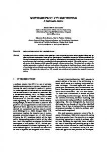
Fig. 2. Change effort distributions from SEL data [22] drawn by the authors.

worst-case settings: the defect correction completion time is at the end of the product project, and DEP is the strongest. We use a probability function for representing an EffDistwcar . We assume that an EffDistwcar has a rightskewed distribution, which is based on the Software Engineering Laboratory (SEL) data subset [22] showing that an effort distribution for error correction is right-skewed as depicted in Fig. 2 (a). The range of the EffDistwcar will be wider than the SEL data distribution, as it represents worst cases of adaptive rework instead of actual effort. It may also have a larger variability than the SEL data distribution, as some residual defects bring multiple changes in a product. With these parameters, the effort of adaptive rework can be determined as follows. The nominal effort of adaptive rework ∆Effar·i (dj ) (in months) caused by the defect dj in the project i is assumed to be represented by the formula ∆Effar·i (dj ) = EffDist−1 wcar·i (p) × WEMi (tdj ) × DEPki × ²,

(1)

where EffDist−1 wcar·i (p) is the inverse function of EffDistwcar for the project i. The probability p is given at random. WEM for the project i is represented with WEMi (tdj ) when the defect dj correction is completed in core asset maintenance phase at the time tdj . DEP between the core assets k and the product i (or core assets i) is represented with DEPki . The parameter ² is 1 if tdj is within the period of the project i. Otherwise, ² is 0. The defect correction completion time td can be determined by applying a Software Reliability Growth Model (SRGM) [23]. Suppose that all residual defects in core assets which bring adaptive rework are detected during core asset maintenance phase. If we draw an SRGM curve during the phase, the defect correction completion time of these defects can be determined by assigning a time to each defect along with the curve depending on reliability growth. An SRGM curve can therefore be considered to represent the organization’s capability for defect detection.

6


Note that the scale of nominal adaptive rework effort is in months, not in person-months. As our simulation model does not consider the number of resources as a parameter, we use nominal effort with a month scale. Though this does not represent the absolute effort overruns, we can compare relative magnitude of the effort. 2.3

Requirements Change Effort Model

To determine the total requirements change effort, we consider as parameters (1) the number of unavoidable critical requirements change requests, (2) the change request arrival time, and (3) the effort of each piece of requirements change. To represent (1) and (2), we consider that a homogeneous Poisson process is applicable. A homogeneous Poisson process is a stochastic process which is defined in terms of the occurrences of events with a known average event occurrence rate. It is widely used to represent discrete event arrivals in simulation studies. However, we do not have any supporting evidence showing that requirements change arrival is represented by using a Poisson process. Actually, some properties of a Poisson process may not conform to the characteristics of requirements change. For example, the probability of two or more requirements changes in a small interval should be essentially 0 if requirements change follows a Poisson process, which does not reflect practical characteristics of requirements change arrival. Though there are several limitations for its application, we use a Poisson process because of its utility for simulation studies. Suppose that RC represents the mean of requirements changes per month. Based on a Poisson process, the interval between any pair of successive requirements changes T follows the probability distribution Pr(T > t) = exp(−RC × t).

(2)

By generating a continuous value ranging from 0 to 1 at random and assigning it to the inverse function of the formula (2) as probability, each interval between two successive requirements change arrivals can be determined. By repeating this calculation until accumulative intervals excess the duration of a product project, the number of requirements changes is bounded. By following the same assumption as adaptive rework effort model, the effort of each requirements change can be determined as follows. The nominal effort of requirements change ∆Effreq·i (rj ) (in months) caused by the change request rj in the project i is assumed to be represented by the formula ∆Effreq·i (rj ) = EffDist−1 wcreq·i (p) × WEMi (trj ),

EffDist−1 wcreq·i (p)

(3)

is the inverse function of the effort distribution probawhere bility function concerning the worst case requirements change for the project i. WEMi (trj ) is in the same notation of formula (1). EffDistwcreq can be considered to have almost the same distribution patterns like Fig. 2 (b). Nurmuliani [5] reported that the average rate of overall requirements change during development lifecycle increased sharply when analysis and documents


7

reviews were being completed, and decreased as the project was getting closer to the end of its lifecycle. We can reflect Nurmuliani’s observation by changing RC during product projects. 2.4

Defect Correction Effort Model

To determine the total defect correction effort, we consider as parameters (1) the number of defects injected during a product project (NDproduct ), (2) the defect correction completion time of these defects, and (3) the effort of each piece of defect correction. NDproduct can be estimated based on estimated product size, process quality, and past experience like NRDcore . The defect correction completion time can be determined by using an SRGM in the same way described in Sect. 2.2. By introducing EffDistwcdc representing worst case defect correction, the nominal effort of defect correction ∆Effdc·i (rj ) (in months) caused by the defect dj in the product project i is assumed to be represented by the following formula: ∆Effdc·i (dj ) = EffDist−1 wcdc·i (p) × WEMi (tdj ),

(4)

where EffDist−1 wcdc·i (p) is the inverse function of EffDistwcdc for the project i. WEMi (trj ) is in the same notation of formula (1). EffDistwcdc can be considered to have almost the same distribution patterns like Fig. 2 (a). 2.5

Model Assumptions

The simulation model relies on the following assumptions. 1. The total effort for product projects is much larger than that for core projects, as stated in Sect. 2.1. 2. Adaptive rework, requirements change, and defect correction occur at the time when the causal defect is detected or the causal requirements change request arrives. Actually, this assumption is not true in practice, as defect correction delay is typically observed [24]. 3. The effort of adaptive rework decreases from EffDistwcar depending on DEP and WEM. The effort of requirements change and defect correction decreases from EffDistwcreq and EffDistwcdc respectively, depending on WEM. These assumptions are partly supported by [17—21]. 4. Adaptive rework for completed projects is not performed even though later defect corrections in dependent core assets may be performed. 5. Adaptive rework, requirements change, and defect correction never inject other defects. This assumption is supported from a differenct viewpoint by the observation in [24] showing that the impact of imperfect defect correction is in practice negligible. 6. There is no relationship between any two pieces of adaptive rework, requirements change, or defect correction.

8

3 3.1


Simulation Results Project Data and Parameters

We have studied a fictional SPL development project for simulation. There are various kinds of team arrangements for SPL development. We suppose that a core project along with its maintenance phase and product projects are conducted concurrently by different teams. We also suppose that product projects are scheduled close together to shorten total cycle time as much as possible. Table 1 shows an overall plan for the project. The first two rows represent when each project is planned to start and finish. The next row “team” represents the team to be assigned for each project. The next four rows represent dependency between core assets and products as well as among core assets. In this project, 4 core assets are scheduled to be developed by the team C independent of the product teams PA and PB, while 10 products by the two product teams concurrently. For example, the product project p3 is planned to start at 4th months, to finish at 7th months, and to be conducted by the team PB. The scheduled total cycle time is 15 months. Table 1. A SPL development project for simulation.

core projects product c1 c2 c3 c4 p1 p2 p3 p4 p5 start (months) 0 2 5 7 2 2 4 5 7 4 7 8 9 finish (months) 2 4 7 9 5 C C C C PA PB PB PA PB team c1 − x x x x x x x x − − x x c2 − − − x c3 − − − − c4

projects p6 p7 8 9 12 11 PA PB x x x x x x

p8 11 13 PB x x x

p9 12 15 PA x x x

p10 13 15 PB x x x

Note that product sizes of core assets and products as well as the number of assigned resources for each project are not considered here, because these factors do not directly affect simulation results in the proposed model. Product size does affect NRDcore and NDproduct as described in Sect. 2.2 and 2.5. DEP might be partly dependent on product size. Several patterns for NRDcore , NDproduct , and RC are studied to explore the research questions. For the other parameters, a fixed value is applied. Table 2 shows the values for these parameters. Regarding to RC, the values in Table 2 are determined based on [5] reporting that mean requirements change per week is approximately between two and three. To reflect Nurmuliani’s observation [5] stated in Sect. 2.3, we divide a product project into halves and assign different values plus and minus two from


9

Table 2. Simulation parameters.

parameters NRDcore NDproduct RC DEP WEM EffDistwcar EffDistwcreq EffDistwcdc

1 4 2 3

pattern no. 2 3 6 8 4 6 6 9 0.5 0.05 to 1.0 μ = 0, σ = 4 μ = 0, σ = 2 μ = 0, σ = 2

remarks 4 10 8 12

for each core asset for each product project (per month) for each product project (per month) a linear model with a factor of 20 the right-hand side of normal distribution the right-hand side of normal distribution the right-hand side of normal distribution

those values for the both part of the project. For example, to represent RC for the pattern no.2, we use 8 for the first half of a project and 4 for the latter half. To generate the distributions of EffDistwcar , EffDistwcreq , and EffDistwcdc , we use the right-hand side half of a normal distribution with the parameters shown in Table 2. The parameters μ and σ for each distribution are determined subjectively to follow almost the same distribution patterns in Fig. 2. The reason why EffDistwcar has a larger standard deviation than the others is that some residual defects bring multiple changes in a product, as described in Sect.2.2. For WEM, a simple linear model ranging from 0.05 to 1.0 is used, which can represent a factor of 20 differences of defect correction cost during design and test [20, 21]. We need to consider another parameter for SRGM to determine defect correction completion time for both adaptive rework and defect correction. Though numerous SRGMs have been proposed in the literature [23], we apply the following simple logarithmic function y = 1 + loga x,

(5)

where y represents cumulative rate of defect correction and x represents normalized duration (0 < x ≤ 1). In this simulation a = 20 is used. It means that, for example, 60% of defects are corrected before 30% of the duration, and 90% of defects before 75% of the duration. 3.2

Result 1: In-Depth View of Simulation Results

Fig. 3 shows an in-depth simulation result under the parameters NRDcore = 4, NDproduct = 2 and RC = 3, which represents when corrective maintenance in core assets and requirements changes occur. One can see that more requirements changes are appeared in the first half of each product project, as we use two different values of RC for first and latter half of the project. Fig.4 shows the effort histograms of generated unplanned work under the same simulation setting in Fig. 3. The shapes of these histograms are all skewed

10


Fig. 3. In-depth view of a simulation result.

Fig. 4. Effort histrograms of generated unplanned work under the same setting in Fig. 3.

to the right, as EffDistwcar , EffDistwcreq , and EffDistwcdc also have right-skewed distributions. The range of Fig.4 (a) is almost the same as those of Fig.4 (b) and (c), though EffDistwcar has larger variability than the others. This is because the effort of each piece of adaptive rework is decreased by multiplying DEP whose value is 0.5. The frequency differences among Fig.4 (a, b, c) depend on the parameters such as NRDcore , NDproduct and RC as well as the number of product projects. With these figures, one can understand how cost overruns are calculated by the simulation model. 3.3

Result 2: Variability of Project Cost Overrun

To explore how much project cost overruns and its variability are expected, we conducted 100-run simulations for several combinations of the parameters. The boxplots in Fig. 5 represent the selected results. The mean and the standard deviation of each combination are shown in the tables below the boxplots. All distributions appeared in Fig. 5 are symmetrical shapes. Note that each y-axis has a different range of nominal cost overruns among boxplots. In Fig. 5 (a, b, c), we have focused on one parameters. That is, we set the value zero for the other two parameters to show the isolated effect on nominal cost overrun. Fig. 5 (d)


11

Fig. 5. Simulation results for estimating nominal project cost overruns (Note: y-scales are different).

represents the simulation results changing all of these parameters at the same time. As compared with Fig. 5 (a, b, c), NRDcore has the smallest impact on nominal cost overruns as well as its variability than the other two parameters, for the studied simulation settings. Meanwhile, RC has the largest impact on nominal cost overrun than the other two parameters. Of course, these results completely rely on what values we have studied for each parameter, which is shown in Table 2. So we can not generalize which parameter has the largest impact on nominal cost overruns. These results only demonstrate the capability of the simulation model to estimate nominal cost overruns as well as its variability based on these parameters. If one gives values of these parameters for a specific project, the possible overruns and its variability can be estimated by the proposed model. Fig. 5 (d) implies that project cost overruns can be held down if requirements volatility and quality are well managed. The mean nominal project cost overruns for the best combinations of these parameters is 3.37 months, while that for the worst case is 13.64 months. As the planned total cycle time is 15 months, the difference between the best and the worst cases are quite significant. The balanced relative estimation error [25] for the mean worst case is 90.1%, which is not regretfully an unrealistic error among typical software projects [26]. It implies that poor management on requirements and quality will result in almost doubled estimation error for the worst case of the studied simulation settings. On the other hand, the differences of variability are relatively small compare to those of the means. For example, the standard deviation of the best case is 0.30 months, while that of the worst case is 0.73 months. It is because that most pieces of unplanned work are distributed among smaller values, even though a lot of unplanned work is generated for the worst case. This result might be different if the assumption no.6 in Sect. 2.5 is changed.

12

4


Model Evaluation

Because of the nature of simulation study, it is impossible to validate all aspects of the proposed simulation model comprehensively. However, the utility of the model can be evaluated by using empirical data, even though it will not demonstrate comprehensive validation. As we are in the process of trying to collect empirical data, we follow some of typical validation aspects for simulation studies [27], which has been applied in our previous work [7]. Conceptual model validity and data validity: The proposed model is considered to be reasonably valid under the assumptions described in Sect. 2.5, because the proposed formulas are partly supported by several empirical observations as stated in Sect. 2. Data validity as input to the model is also supported by these empirical observations in terms of determining effort distributions. However, there are some limitations of the model, which is discussed in Sect. 5.1. Operational validity: In general, operational validity is difficult to assess when no observable problem entity is available. In such a case, comparison to other models is one of meaningful approaches to validate a simulation model [27]. However, this approach is not applicable in this case, because both COCOMO II [12] and COPLIMO [13], a COCOMO II based cost estimation model for SPL development, do not produce variability of estimated effort. These models have a lot of parameters such as effort multipliers, but these parameters are deterministic but not stochastic. In addition, the proposed model is not capable of being compared to these models, as the model uses nominal cost scale. Sensitivity analysis is another useful approach to demonstrate operational validity of the model, which we have already discussed in Sect. 3.3. It can be considered that the model has reasonable validity, but some limitations still exist. Another possible approach is to evaluate the generated adaptive rework by the simulation program rather than total cycle time. By comparing the distributions of the generated adaptive rework in Fig. 4 to the change effort distribution from the SEL data in Fig. 2, both distributions can be subjectively judged to be similar. At least, we can conclude that the simulation model is capable of producing reasonable adaptive rework distributions.

5 5.1

Discussion and Related Work Limitation of the Model

One of the most important limitations of this study is that the proposed model uses nominal cost scale but absolute cost scale. That is, the model estimates cost overruns in month scale but not in person-month scale. This limitation comes from the lack of considerations for resources and product size. In addition, the model does not consider unplanned work during core asset development phase. Matured SPL development tends to have more effort on core projects rather than product projects [16], so this limitation should be overcome to increase applicability of the model. Now we are in the process of enhancing the simulation model to overcome these limitations and some assumptions as well.


13

Another arguable assumption in this model is the usage of DEP. We assume that the effort of a piece of unplanned work decreases linearly from worst-case effort by multiplying DEP. We do not have any supporting evidence for this assumption at this moment. We might say that this assumption is not very unrealistic by carefully looking at the generated unplanned work distributions. In addition, we do not have any specific method to caliblate DEP. It might reflect attributes such as coupling between core components and product components, number of dependent product components reusing a core component, and inheritance depth between core and product components. Those attributes and measured values have to be translated into DEP and calibrated by checking generated adaptive rework distributions like Fig. 4 (a). 5.2

Related Work

Software process modeling approaches can be categorized into the following three types [28]: analytical models such as COCOMO II [12], continuous simulations such as system dynamics models [29, 30], and discrete-event simulations [31]. Some studies use a combination of those approaches [14, 28, 32]. The proposed model is a discrete-event simulation. Discrete-event simulation models are suitable for detailed analyses of the process and project performance, while continuous simulation models are useful to represent effects of feedback and changes in a continuous fashion [33]. As the proposed model represents sequential events concerning defects and requirements change requests, the use of a discrete-event simulation model is reasonable. Several studies have appeared in the literature on estimating the benefits of SPL development [13, 34, 35]. These studies use more macro-level analytical models than our model. The primary purpose of the studies [34, 35] is for estimating the return on investment of SPL development compared with non-SPL development. COPLIMO [13] is a deterministic cost estimation model for SPL and does not represent uncertainty, as well as COCOMO II [12]. COCOMO-U [15] introduces uncertainty into COCOMO II, but does not mention how the model can be applied to SPL development. Chen et al. proposed a discrete-event SPL process simulator using COPLIMO as their cost model [14]. Schmid et al. studied SPL planning strategies through deterministic simulations [2]. These two studies have similar research questions to ours. However, these studies do not explicitly use factors such as NRDcore , NDproduct , DEP, and requirements volatility. They are also not capable of calculating the level of risk of estimated effort under uncertainty, as they are based on deterministic simulation models.

6

Conclusions

In this paper, we proposed a stochastic simulation model for estimating nominal project cost overruns and its variability in time-boxed SPL development, based

14


on our previous model. Simulation results demonstrate that the model is capable of estimating reasonable nominal cost overruns and its variability. We have shown that poor management on requirements and quality will result in almost doubled estimation error, for the studied settings. The model has been partially validated by comparing generated unplanned work to actual change effort, which consequently demonstrates the validity of estimated project cost overruns. Our immediate future work is to enhance the model to overcome limitations and assumptions, consider calibration of the parameters, and to validate the model by using empirical project data. We are now working on these issues. Acknowledgments. This study was partially supported by the Ministry of Education, Science, Sports and Culture, Grant-in-Aid for Young Scientists (B), 16700042, 2005. NICTA is funded through the Australian Government’s Backing Australia’s Ability initiative, in part through the Australian Research Council. The third author was working with NICTA when this paper was produced.

References 1. Clements, P., Northrop, L.M.: Software Product Lines: Practices and Patterns. Addison-Wesley, MA (2001) 2. Schmid, K., Biffl, S.: Systematic management of software product lines. Softw. Process Improve. Pract. 10 (2005) 61—76 3. Genuchten, M.v.: Why is software late? an empirical study of reasons for delay in software development. IEEE Trans. Softw. Eng. 17(6) (1991) 4. Subramanian, G.H., Breslawski, S.: An empirical analysis of software effort estimate alterations. J. Systems and Software 31(2) (1995) 135—141 5. Nurmuliani, N., Zowghi, D., Fowell, S.: Analysis of requirements volatility during software development life cycle. In: Proc. 2004 Australian Softw. Eng. Conf. (ASWEC’04). (2004) 6. Dijkstra, E.: Notes on structured programming. In Dahl, O.J., Dijkstra, E., Hoare, C.A.R., eds.: Structured Programming. Academic Press, London (1972) 7. Nonaka, M., Zhu, L., Babar, M.A., Staples, M.: Project delay variability simulation in software product line development (to appear). In: Proc. Intl. Conf. Software Process (ISCP). (2007) 8. IEEE: Ieee std. 1219-1998, ieee standard for software maintenance (1998) 9. Jørgensen, M., Moløkken, K.: Reasons for software effort estimation error: Impact of respondent role, information collection approach, and data analysis method. IEEE Trans. Softw. Eng. 30(12) (2004) 993—1007 10. Jørgensen, M.: Realism in assessment of effort estimation uncertainty: It matters how you ask. IEEE Trans. Softw. Eng. 2004(30) (2004) 209—217 11. Procaccino, J.D., Verner, J.M.: Software project managers and project success: An exploratory study. J. Systems and Software 79 (2006) 1541—1551 12. Boehm, B.W., Abts, C., Brown, A.W., Chulani, S., Clark, B.K., Horowitz, E., Madachy, R., Reifer, D., Steece, B.: Software Cost Estimation with COCOMO II. Prentice Hall (2000) 13. Boehm, B.W., Brown, A.W., Madachy, R., Yang, Y.: A software product line life cycle cost estimation model. Proc. 2004 Intl. Symp. Empirical Softw. Eng. (ISESE’04) (2004) 156—164


15

14. Chen, Y., Gannod, G.C., Collofello, J.S.: A software product line process simulator. Softw. Process Improve. Pract. 11 (2006) 385—409 15. Yang, D., Wan, Y., Tang, Z., Wu, S., He, M., Li, M.: Cocomo-u: An extension of cocomo ii for cost estimation with uncertainty. Lecture Notes in Computer Science 3966 (2006) 132—141 16. Bosch, J.: Maturity and evolution in software product lines: Approaches, artefacts and organization. In: Proc. 2nd Intl. Conf. Softw. Product Lines. (2002) 257—271 17. Epping, A., Lott, C.M.: Does software design complexity affect maintenance effort? In: Proc. 19th Softw. Eng. Workshop. (1994) 297—313 18. Bocco, M.G., Moody, D.L., Piattini, M.: Assessing the capability of internal metrics as early indicators of maintenance effort through experimentation. J. Software Maintenance and Evolution 17(3) (2005) 225—246 19. Ramanujan, S., Scamell, R.W., Shah, J.R.: An experimental investigation of the impact of individual, program, and organizational characteristics on software maintenance effort. J. Systems and Software 54 (2000) 137—157 20. Kan, S.H., Dull, S.D., Amundson, D.N., Lindner, R.J., Hedger, R.J.: As/400 software quality management. IBM Systems Journal 33(1) (1994) 62—88 21. Remus, H.: Integrated software validation in the view of inspections / reviews. In: Proc. Symposium on Softw. Validation, Elsevier (1983) 57—64 22. SEL: Sel (software engineering laboratory) data. http://www.cebase.org (1997) 23. Musa, J.D.: Software Reliability Engineering. Osborne/McGraw-Hill (1998) 24. Defamie, M., Jacobs, P., Thollembeck, J.: Software reliability: assumptions, realities and data. In: Proc. 1999 Intl. Conf. Softw. Maintenance (ICSM’99). (1999) 337—345 25. Miyazaki, Y., Takanou, A., Nozaki, H., Nakagawa, N., Okada, K.: Method to estimate parameter values in software prediction models. Inf. Softw. Technol. 33(3) (1991) 239—243 26. Moløkken, K., Jørgensen, M.: A comparison of software project overruns—flexible versus sequential development models. IEEE Trans. Softw. Eng. 31(9) (2005) 754—766 27. Sargent, R.G.: Validation and verification of simulation models. Proc. 31st Conf. Winter Simulation (1999) 39—48 28. Donzelli, P.: A decision support system for software project management. IEEE Software 23(4) (2006) 67—75 29. Abdel-Hamid, T., Madnick, S.: Software Project Dynamics- An Integrated Approach. Prentice-Hall, Englewood Cliffs, NJ (1991) 30. Calavaro, G.F., Basili, V.R., Iazeolla, G.: Simulation modeling of software development process. In: Proc. 7th European Simulation Symposium. Soc. for Computer Simulation. (1995) 31. Antoniol, G., Cimitile, A., Lucca, G.A., Penta, M.: Assessing staffing needs for a software maintenance project through queuing simulation. IEEE Trans. Softw. Eng. 30(1) (2004) 43—58 32. Martin, R., Raffo, D.: Application of a hybrid process simulation model to a software development project. J. Systems and Software 59(3) (2001) 237—246 33. Kellner, M.I., Madachy, R.J., Raffo, D.M.: Software process simulation modeling: Why? what? how? J. Systems and Software 46(2-3) (1999) 113—122 34. Cohen, S.: Predicting when product line investment pays. Technical Report Techinical Report CMU/SEI-2003-TN-017, Software Engineering Institute, Carnegie Mellon University (2003) 35. B¨ ockle, G., Clements, P., McGregor, J.D., Muthig, D., Schmid, K.: Calculating roi for software product lines. IEEE Software 21(3) (2004) 32—38

Project Cost Overrun Simulation in Software Product Line Development

Project Cost Overrun Simulation in Software Product Line Development

Suggest Documents