Projection Operator Approach to Spin Diffusion in the Anisotropic Heisenberg Chain at High Temperatures Robin Steinigeweg1, ∗ and Roman Schnalle2, † 1
arXiv:1006.4511v1 [cond-mat.stat-mech] 23 Jun 2010
Institute for Theoretical Physics, Technical University Braunschweig, Mendelsohnstr. 3, D-38106 Braunschweig, Germany 2 Department of Physics, University Bielefeld, Universit¨ atsstr. 25, D-33615 Bielefeld, Germany (Dated: June 24, 2010) We investigate spin transport in the anisotropic Heisenberg chain in the limit of high temperatures (β → 0). We particularly focus on diffusion and the quantitative evaluation of diffusion constants from current autocorrelations as a function of the anisotropy parameter ∆ and the spin quantum number s. Our approach is essentially based on an application of the time-convolutionless (TCL) projection operator technique. Within this perturbative approach the projection onto the current yields the decay of autocorrelations to lowest order of ∆. The resulting diffusion constants scale as ∆−2 in the Markovian regime ∆ ≪ 1 (s = 1/2) and as ∆−1 in the highly non-Markovian regime above ∆ ∼ 1 (arbitrary p s). In the latter regime the dependence on s appears approximately as an overall scaling factor s(s + 1) only. These results are in remarkably good agreement with diffusion constants for ∆ > 1 which are obtained directly from the exact diagonalization of autocorrelations or have been obtained from non-equilibrium bath scenarios. PACS numbers: 05.60.Gg, 05.30.-d, 05.70.Ln
Transport in one-dimensional quantum systems has been a topic of theoretical investigations since at least the 1960s [1, 2]. Even nowadays there is an ongoing and still increasing interest in understanding the transport phenomena in such systems, including their dependence on length scales and temperature [3–15]. Much work has been devoted to a rather qualitative classification of the emerging transport types into either non-normal ballistic or normal diffusive behavior. In this context the crucial mechanisms for the emergence of pure diffusion have been intensively studied and in particular non-integrability or quantum chaos are frequently discussed w.r.t. their role as an at least necessary prerequisite [12–14]. Spin chains are a central issue of research with a considerable focus on spin transport in the anisotropic Heisenberg chain, in particular on the case s = 1/2 [3–13]. In that case there still is an unsettled debate about the concrete range of anisotropies where the dynamics at finite temperatures is indeed diffusive [3–5]. However, even if the diffusive range of anisotropies was definitely known, the question about the quantitative value of the diffusion coefficient arises naturally. In fact, this question is as challenging as the proof of diffusion as such. Because the majority of all available approaches to transport has to deal more or less with finite quantum systems, signatures of diffusion in the thermodynamic limit may not be observed, e.g., due to large mean free paths, even in the limit of high temperatures. For these temperatures diffusion coefficients can be found in the literature for s = 1 and the isotropic point [1, 2, 15] and for s = 1/2 and a narrow window of large anisotropies above the isotropic point [7–11] solely. On that account there is an urgent need for a much more comprehensive picture of diffusion constants.
In this work we intend to make an essential step towards such a picture at high temperatures. To this end we focus on the quantitative evaluation of diffusion constants from current autocorrelations, either directly or perturbatively by the use of projection operator techniques, see Refs. 16–19. Within this perturbative approach the projection onto the current yields the decay of autocorrelations to lowest order of the anisotropy parameter. The resulting diffusion constant is a smooth function of the anisotropy and agrees well with the above ones from the literature for large anisotropies, i.e., at the upper boundary of the expected range of validity. This agreement also supports the validity of the perturbative approach in the limit of small anisotropies, if transport is indeed diffusive. The anisotropic Heisenberg chain (XXZ model) may be ˆ =H ˆ 0 + ∆ Vˆ , described by a Hamiltonian of the form H where Hˆ0 and Vˆ are given by ˆ0 = J H
N X
µ=1
sˆxµ sˆxµ+1 + sˆyµ sˆyµ+1 ,
Vˆ = J
N X
sˆzµ sˆzµ+1 (1)
µ=1
with periodic boundary conditions. Here, J denotes the nearest neighbor coupling strength, ∆ the anisotropy, N the number of sites, and the operators sˆiµ (i = x, y, z) represent the standard spin matrices (w.r.t. site µ) for the spin quantum number s. For thepclarity of later notations we define the abbreviation s˜ ≡ s(s + 1). The Einstein relation σdc = χ D connects the spin (dc) conductivity σdc and the spin diffusion constant D via the static susceptibility χ. Therefore the spin diffusion constant according to linear response theory (LR) [20] reads in the limit of high temperatures (β → 0) Z t β dt′ C(t′ ) , (2) D = lim D(t) , D(t) = t→∞ χ dimH N 0
2 where χ = 1/3 β s˜2 , dimH = (2s + 1)N , and the spin current autocorrelation function is given by ˆ Jˆ(0)} , C(t) = Tr{J(t)
Jˆ = J
N X
sˆxµ sˆyµ+1 − sˆyµ sˆxµ+1 (3)
µ=1
with the initial value Tr{Jˆ2 } = 2/9 J 2 s˜4 dimH N . For s = 1/2 the infinite time integral in Eq. (2) diverges for ˆ 0 , J] ˆ = 0 [21]. It also diverges, whenever ∆ = 0 due to [H there is only partial conservation, i.e., a non-zero Drude weight. Finite Drude weights indicate ballistic transport at the infinite time scale but are commonly expected to vanish in the thermodynamic limit for the non-integrable cases s > 1/2 [15]. For the integrable case s = 1/2 Drude weights are widely expected to vanish for ∆ > 1 [6, 7], while they may already be zero for ∆ = 1 [3, 4] or even for all 0 < ∆ < 1 [5]. Apart from the common LR picture, the time-dependent diffusion coefficient D(t) according to Eq. (2) can be also connected to the time evolution of the spatial variance of an initially inhomogeneous non-equilibrium density, see Refs. 10, 11. Within this picture the density dynamics is diffusive at a certain time, respectively length scale, if D(t) is constant at that scale. Such a scale may exist, even if D(t) eventually diverges in the infinite time limit, i.e., despite finite Drude weights. We thus do not focus only on the infinite time limit, but investigate the full time dependence of D(t), too.
3
diff. const. D(t) / √s(s+1) [J]
s=1/2 s=1 s=3/2 s=2
2
1
0 0
5
10
15
20
time t √s(s+1) [1/J] FIG. 1: The time dependence of the spin diffusion constant D(t) in the limit of high temperatures (β → 0), as obtained directly from exact diagonalization. The data is displayed for the anisotropy parameter ∆ = 1.5 and for the spin quantum numbers s = 1/2 (N = 20), s = 1 (N = 12), s = 3/2 (N = 9), and s = 2 (N = 8). The data in the inset is shown for the spin quantum number s = 1/2 and for various chain lengths N = 8, 10, . . . , 20.
A possible strategy for the analysis of the dependence of D(t) on time is the direct application of numerically exact diagonalization (ED). Of course, ED is restricted
to a rather limited range of N , even if all symmetries are taken into account, e.g., translation, rotation about the z-axis [22]. But finite N effects are often less pronounced at finite time scales. In Fig. 1 we show D(t) at such time scales for ∆ = 1.5 and the maximum N which is available to us for a certain s: D(t) firstly increases at short times t . 2/(J s˜) and then becomes approximately constant at intermediate times, i.e., a “plateau” with a height of about D ≈ 0.7 J s˜ is formed here. D(t) finally increases again due to non-zero Drude weights for finite N . But in the thermodynamic limit Drude weights are expected to vanish for ∆ = 1.5 and each s. Furthermore, the height of the plateau does not change with N , while its width gradually increases, see Fig. 1 (inset). The height of this plateau consequently is a reasonable suggestion for the concrete value of the diffusion coefficient [10, 11]. In fact, for s = 1/2 the value D ≈ 0.6 J is in remarkably good agreement with non-equilibrium bath scenarios [8, 9]. Analogously, the concept of plateaus allows to suggest further values of the diffusion coefficient for anisotropy parameters above ∆ ∼ 1.4, see Fig. 3 (squares). Here, the dependence of D on s appears approximately as a scaling factor s˜. For anisotropy parameters below ∆ ∼ 1.4 the suggestion of diffusion coefficients is not possible, because Drude weights become dominant and plateaus disappear for finite N . Plateaus appear only, if contributions from the Drude weight and the regular part are well-balanced, at least to some degree. However, plateaus are also not visible, if both contributions are treated separately from each other [11]. Another strategy for the analysis of the time evolution of C(t), respectively D(t) is provided by an application of the time-convolutionless (TCL) projection operator technique [16, 17]. This technique, and the well-known Nakajima-Zwanzig (NZ) method [18, 19], are commonly applied in order to describe the reduced dynamics for a set of relevant variables. Their application essentially ˆ =H ˆ 0 + ∆ Vˆ and requires a Hamiltonian of the form H ˆ 0 (or a the commutation of the relevant variables with H ˆ comparatively slow dynamics w.r.t. H0 ). Although both methods are well-established approaches in the context of open quantum systems, the following approach to current autocorrelation functions in closed quantum systems is an uncommon concept. However, in this context NZ is very similar to the more common Mori-Zwanzig memory matrix formalism, see Ref. 14. But a “Mori-TCL” variant does not exist, of course. The above-mentioned set of relevant variables is specified by the definition of a suitable projection (super)operator P which projects out the relevant part of an operator ρˆ(t). (This operator does not need to be a density matrix in the strict sense.) To this end we define 1 Aˆ ≡ Tr{Jˆ2 }− 2 Jˆ ,
P ρ(t) ≡ Tr{Aˆ ρˆ(t)} Aˆ ,
(4)
where the normalized current operator Aˆ is introduced in order to satisfy the property P 2 = P of a projection
d C(t) = −R(t) C(t) , dt
R(t) =
∞ X
∆2i R2i (t)
(5)
i=1
and avoids the often troublesome time-convolution which appears in the NZ variant [16, 17]. The time-dependent rate R(t) is given in terms of a systematic perturbation expansion in powers of ∆. (All odd orders of ∆ vanish for this and many other quantum systems.) The truncation of R(t) to lowest order of ∆ reads 2
R(t) ≈ ∆
Z
t
dt′ f (t′ )
(6)
0
2
s=1/2 s=1 s=3/2 s=2
2
(super)operator. For the initial condition ρˆ(0) = Aˆ the TCL technique routinely yields a homogenous differential equation for ˆ AˆI (t)}. Here, the actual expectation value a(t) ≡ Tr{A(t) ˆ the index I of AI (t) denotes the interaction picture, i.e., ˆ 0 . Since C(t) ∝ a(t) for the Heisenberg picture w.r.t. H ˆ ˆ ˆ ˆ AI (t) = A (or AI (t) ≈ A at a pertinent time scale [21]), the TCL equation is identical for C(t) in that case. It then reads
TCL rate R(t) / √s(s+1) [∆ J]
3
1
0 0
5
10
15
time t √s(s+1) [1/J] FIG. 2: The time dependence of the decay rate R(t), as given by Eq. (6). The data is shown for the spin quantum numbers s = 1/2 (N = 20), s = 1 (N = 12), s = 3/2 (N = 9), and s = 2 (N = 8). The data in the inset is displayed for the spin quantum number s = 1/2 and for various chain lengths N = 8, 10, . . . , 20. The extracted plateau height for s > 1/2 is indicated (arrow).
with the two-point correlation function ˆ Vˆ ]I (t) ı[J, ˆ Vˆ ]I (0) } , f (t) = Tr{Jˆ2 }−1 Tr{ ı[J,
(7)
where the above index I indicates again the Heisenberg ˆ 0 . In general this lowest order truncation picture w.r.t. H is expected to be justified for small ∆ (and short t). Even though the incorporation of higher order corrections is in principle possible, their concrete evaluation is an almost impossible task, both from an analytical and numerical point of view. The concrete evaluation of the lowest order truncation for R(t) in Eq. (6) is feasible. Moreover, this evaluation may ˆ 0 can be brought in diagonal be done analytically, if H form, e.g., via the Jordan-Wigner transformation onto non-interacting spinless fermions for s = 1/2. However, since the expression for R(t) still takes on a non-trivial form after such a transformation, it may possibly have to be evaluated numerically at the end. We thus directly evaluate R(t) in Fig. 2 numerically by the use of ED, similarly as done in Refs. 13, 14. There is an apparent similarity between Figs. 1 and 2, even though completely different quantities are shown. In particular a constant rate R ≈ 0.67 ∆2 J s˜ may be read off from the height of the plateau at intermediate times, at least for s = 1/2. Of course, for s > 1/2 the plateau is not developed as clearly for finite N . But the respective R(t)-curves have converged completely for short times t . 2/(J s˜) solely. We hence assume a constant rate R in that case also, e.g., as given by the height of the local maximum at such times, see Fig. 2 (arrow). Obviously, this assumption implies a positive R, i.e., we expect that TCL does simply not predict Drude weights to lowest order, see below. However, in principle R(t) may become
zero in the long-time limit. The above assumption is relevant only in the Markovian limit of long relaxation times, i.e., small ∆. In that limit the rate R(t) can be replaced by the constant value R and lowest order TCL consequently predicts the exponential decay C(t) = C(0) exp(−R t), cf. Eq. (5). The diffusion constant in Eq. (2) eventually scales as D ∝ R−1 ∝ ∆−2 , e.g., as generally expected from a Boltzmann equation approach to the same question. The Markovian limit of long relaxation times concretely turns out to be realized for ∆ ≪ 1, see Fig. 3. However, in that limit the resulting diffusion constants for s > 1/2 have to be understood in terms of an upper boundary. Since AˆI (t) ≈ Aˆ does not hold true for long relaxation times, a back-transform from the interaction picture becomes necessary in order to obtain C(t) from a(t). Because we do not perform this back-transform due to its unavailability, we only consider the contribution ˆ 0 , i.e., C(t) from Vˆ and neglect any contribution from H probably decays too slowly. Obviously, C(t) decays too ˆ 0 contributes, i.e., for ∆ = 0. slowly, if exclusively H For small ∆ there is no substantial difference between the predictions of lowest order TCL and NZ. But the situation changes for large ∆, when relaxation times are short and non-Markovian effects become relevant, i.e., the initial increase of the rate R(t) at short times, see Fig. 2. At such times the R(t)-curve has well converged already for each s and additional assumptions like the one above are not required here. Since the initial increase appears to be approximately linear, lowest order TCL predicts a Gaussian decay in the highly non-Markovian limit. As a consequence the diffusion constant scales as
4 is reasonably suggested by lowest order TCL, e.g., as displayed for s = 1/2 in Fig. 3. We sincerely thank Wolfram Brenig, J¨ urgen Schnack, and Jochen Gemmer for fruitful discussions. We further gratefully acknowledge financial support by the Deutsche Forschungsgemeinschaft, one of us (RST) through FOR 912.
s=1/2 s=1 s=3/2 s=2
2
2
diff. const. D ∆ /√s(s+1) [J]
3
1
∗
0
†
0
0.5
1
1.5
2
anisotropy parameter ∆ FIG. 3: The spin diffusion constant D as a function of the anisotropy parameter ∆ in the limit of high temperatures (β → 0), as predicted by TCL to lowest order of ∆, for the spin quantum numbers s = 1/2, . . . , 2 (curves). Further data from exact diagonalization (squares, s ≥ 1/2) and from the literature are indicated: Ref. 7 (rhombus, s = 1/2), Refs. 8, 9 (triangles, s = 1/2), and Refs. 1, 2, 15 (circle, s = 1). Curves for s > 1/2 and ∆ ≪ 1 have to be understood in terms of an upper boundary. (D is located somewhere below, e.g., as sketched by the filled area.)
D ∝ ∆−1 now. The highly non-Markovian limit of very short relaxation times turns out to be concretely realized for anisotropies above ∆ ∼ 1, see Fig. 3. For s > 1/2 the diffusion constants according to lowest order TCL in Fig. 3 are in excellent agreement with the results from ED for ∆ > 1 in Fig. 1. Furthermore, these diffusion constants are in good agreement with results for ∆ = 1 in the literature (standard frequency moments analysis, microcanonical Lanczos method [1, 2, 15]). For s = 1/2 there is a deviation on the order of 20% between diffusion coefficients according to lowest order TCL and results for ∆ ∼ 1.5 from ED in Fig. 1 or the literature (non-equilibrium bath scenarios [8, 9]). Such a deviation probably arises from the neglection of all higher order corrections which are more important for s = 1/2. Of course, the above agreement also supports the validity of lowest order TCL for s = 1/2 and ∆ ≪ 1, e.g., the usual range of application for a perturbation theory. But one has to keep in mind that this perturbation theory is generally restricted to small ∆ and short t as well. The restriction becomes manifest, since we expect that TCL does simply not predict Drude weights to lowest order, i.e., the non-decaying character of C(t) essentially is a higher order effect, as known for large ∆. Consequently, lowest order TCL can be valid at all t only, if Drude weights eventually vanish in the thermodynamic limit. On that account we may finally conclude as follows: Whenever there is spin diffusion in the XXZ model at high temperatures, either at a finite or the infinite time scale, we expect that the respective diffusion coefficient
[1] [2] [3] [4] [5] [6] [7] [8] [9] [10] [11] [12] [13] [14] [15] [16] [17] [18] [19] [20]
[21]
[22]
Electronic address:
[email protected] Electronic address:
[email protected] D. L. Huber and J. S. Semura, Phys. Rev. 182, 602 (1969). D. L. Huber, J. S. Semura, and C. G. Windsor, Phys. Rev. 186, 534 (1969). X. Zotos, Phys. Rev. Lett. 82, 1764 (1999). J. Benz, T. Fukui, A. Kl¨ umper, and C. Scheeren, J. Phys. Soc. Jpn. Suppl. 74, 181 (2005). J. Sirker, R. G. Pereira, and I. Affleck, Phys. Rev. Lett. 103, 216602 (2009). F. Heidrich-Meisner, A. Honecker, D. C. Cabra, and W. Brenig, Phys. Rev. B 68, 134436 (2003). P. Prelovˇsek, S. El Shawish, X. Zotos, and M. Long, Phys. Rev. B 70, 205129 (2004). M. Michel, O. Hess, H. Wichterich, and J. Gemmer, Phys. Rev. B 77, 104303 (2008). ˇ T. Prosen and M. Znidariˇ c, J. Stat. Mech. 2009, P02035 (2009). R. Steinigeweg, H. Wichterich, and J. Gemmer, EPL 88, 10004 (2009). R. Steinigeweg and J. Gemmer, Phys. Rev. B 80, 184402 (2009). H. Castella, X. Zotos, and P. Prelovˇsek, Phys. Rev. Lett. 74, 972 (1995). P. Jung and A. Rosch, Phys. Rev. B 76, 245108 (2007). P. Jung, R. W. Helmes, and A. Rosch, Phys. Rev. Lett. 96, 067202 (2006). J. Karadamoglou and X. Zotos, Phys. Rev. Lett. 93, 177203 (2004). S. Chaturvedi and F. Shibata, Z. Phys. B 35, 297 (1979). H.-P. Breuer and F. Petruccione, The Theory of Open Quantum Systems (Oxford University Press, New York, 2007). S. Nakajima, Progr. Theor. Phys. 20, 948 (1958). R. Zwanzig, J. Chem. Phys. 33, 1338 (1960). R. Kubo, M. Yokota, and S. Hashtisume, Statistical Physics II: Nonequilibrium Statistical Mechanics, vol. 31 of Solid State Sciences (Springer, New York, 1991), 2nd ed. P z 2 z ˆ 0 , J] ˆ ∝ [H sµ ) (ˆ sµ+1 − sˆzµ−1 ) is non-zero for s > 1/2 µ (ˆ and numerics also indicates a (partial) decay of C(t) at a time scale t ≫ 2/(J s˜). R. Schnalle and J. Schnack, Phys. Rev. B 79, 104419 (2009).