Engineering Structures 22 (2000) 1677–1689 www.elsevier.com/locate/engstruct
Proof load testing for bridge assessment and upgrading Michael H. Faber a, Dimitri V. Val b
b,*
, Mark G. Stewart
b
a COWI, Consulting Engineers and Planners AS, Lyngby, DK-2800, Denmark Department of Civil, Surveying and Environmental Engineering, The University of Newcastle, Newcastle, NSW 2308, Australia
Received 27 April 1999; received in revised form 27 September 1999; accepted 10 November 1999
Abstract Bridge deterioration with time and ever increasing traffic loads raise concerns about reliability of aging bridges. One of the ways to check reliability of aging bridges is proof load testing. A successful proof load test demonstrates immediately that the resistance of a bridge is greater than the proof load. This reduces uncertainty in the bridge resistance and so increases the bridge reliability. The paper considers a reliability-based calibration of intensities of proof loads for aging bridges to verify either an existing or increased load rating taking into account possible bridge deterioration. Intensities of proof loads are calibrated based on a consistent target reliability index. The influence of test risk, dead to live load ratio, and uncertainties associated with dead and live loads and bridge resistance is considered. The results presented in the paper relate to short and medium span bridges. 2000 Elsevier Science Ltd. All rights reserved. Keywords: Bridges; Proof loads; Time dependent reliability
1. Introduction It is quite evident that the bridge population in the US, Canada, Europe, Australia and elsewhere is aging. This is due to aging local road bridges and the large expansion of highways built during the post-war boom era of the 1950s to 1970s. For example, in Australia, over 60% of bridges for local roads are over 50 yr old and approximately 55% of all highway bridges are over 20 yr old. These figures are typical of other countries also. The incidence of structural deterioration increases with bridge age due to corrosion, fatigue, wear and tear and other forms of material property degradation. During this same period vehicle loads and legal load limits have been steadily increasing. Aging bridges subject to increasing legal load limits mean that existing bridges often fail to satisfy structural requirements as specified for new bridges. There is obviously a strong financial incentive that existing bridges be conserved and their remaining service life extended. In general, bridge assessment is conducted to either: * Corresponding author. Current address: School of Engineering, James Cook University, Townsville, QLD 4811, Australia. Tel.: + 617-4781-4722; fax: + 61-7-4775-1184. E-mail address:
[email protected] (D.V. Val).
(i) confirm an existing load rating (if bridge deterioration is observed or suspected), or (ii) increase a load rating. Analytical or predictive approaches to determining load ratings are well documented and widely used. However, such approaches may be overly conservative. For example, the actual load carrying capacity of a bridge is often higher than the predicted capacity, this may be due to system effects, load redistribution, contribution of non-structural elements and bearings not behaving in an ‘idealised’ manner [1,2]. It is desirable that the assessment of existing bridges not be overly conservative since such an approach may result in the replacement of bridges that are in fact ‘satisfactory’. As such, a diagnostic or proof load test may be more appropriate if 앫 analytical analyses produces an unsatisfactory load rating; or 앫 analytical analysis is difficult to conduct due to deterioration or lack of documentation. A diagnostic test may be used to verify or refine analytical or predictive structural models, whilst a proof load test is used to assess the actual load carrying capacity of a bridge. A successful proof load test demonstrates immediately that the resistance of the bridge is greater than the proof load. As a result, this reduces uncertainty
0141-0296/00/$ - see front matter 2000 Elsevier Science Ltd. All rights reserved. PII: S 0 1 4 1 - 0 2 9 6 ( 9 9 ) 0 0 1 1 1 - X
1678
M.H. Faber et al. / Engineering Structures 22 (2000) 1677–1689
associated with the resistance of the bridge and so increases its reliability [3]. Moreover, a proof load test may provide additional useful information about bridge properties and performance. However, extensive proof load testing programs are very costly. For example, proof load testing of bridges in New South Wales, Australia, can cost up to A$110,000 per bridge or 6% of the bridge replacement cost [4]. Given the large costs involved it is surprising that proof load testing procedures are not well documented [5]. It should be recognised also that there is a risk that the bridge will be damaged or not survive a proof load test (referred to herein as test risk) and so proof load testing may not always be cost-effective [6]. The present paper presents a reliability-based method (i.e. reliability is used as the measure of structural performance) to determine the target proof load. Previous reliability studies [5,7,8] in this area are quite limited and have (i) ignored the risks associated with failure of a bridge during the load test—this is referred to herein as the ‘test risk’ (although Moses et al. [8] have considered test risk); (ii) assumed bridge reliabilities were not influenced by the timing of the proof load test; and (iii) ignored the effects of structural deterioration. Clearly, these are not realistic assumptions. Stewart and Val [6] improved this previous work by developing a probabilistic framework that considers bridge age, deterioration, magnitude of proof loads, test risk, updated bridge reliability (for prior service loading and proof loading) and associated decision-making applications such as a risk–cost–benefit analysis. The present paper considers a practical implementation of such a probabilistic approach, in this case by using reliability-based methods to propose target proof loads to either verify an existing load limit or assess a bridge for an increased load limit, for non-deteriorated or deteriorated bridges. In this approach, target proof loads are calibrated from a consistent target reliability index and the influence of test risk, dead to live load ratio, dead and live loading variability, and resistance modelling uncertainty is considered. A risk–cost–benefit analysis is not considered herein. The results presented herein relate to short and medium span bridges.
reliability index. As such, bridge reliability (or safety) is influenced by resistance and loading variability. However, the observation that a bridge survives a proof load test indicates only the minimum load-carrying capacity of the bridge—it does not reveal the actual bridge capacity and also does not provide a meaningful measure of the safety of the bridge. To be consistent with LRFD principles, an assessment procedure should show that the post-test bridge reliability is acceptable. Consequently, decisions related to bridge assessment are based on uncertain or incomplete information. Deterministic approaches are not efficient for decisions taken under uncertainty since such decisions tend to be conservative and based on ‘prudent pessimism’ or ‘worst case’ scenarios. Reliability (or probabilistic) analysis includes information from all resistance and loading variables influencing the assessment process (not just point estimates) and so provides a rational criterion for the comparison of the likely consequences of decisions taken under uncertainty. The initial stage of a bridge assessment is to estimate the reliability of the existing bridge, such a reliability analysis should consider the following uncertainties:
2. Reliability considerations for proof load testing
Information regarding the reliability of the existing bridge is also needed to determine the target proof load. After the application of a target proof load the bridge reliability can again be updated. This occurs since the lower tail of the distribution of structural resistance is truncated at the target proof load, resulting in a higher bridge reliability. Although this could be at the expense of an unacceptable test risk. Note that an additional source of uncertainty can arise since the proof load may not always be applied in a correct and controlled manner. After a proof load test it is often of interest to deter-
The carrying out of a proof load test is a complicated and often bridge-specific procedure specified by highway agency, state or national guidelines. It is beyond the scope of the present paper to describe such procedure; however, it can be found elsewhere [2,9]. The design of new bridges is increasingly being based on LRFD or limit state design principles [10,11] in which all ‘typical’ bridges have relatively uniform reliabilities and that these reliabilities exceed a target
앫 representation of real structures by idealised prediction models (model errors); 앫 inherent variability of material properties; 앫 variability in workmanship, element dimensions and environmental conditions; 앫 spatial variations in material and other properties; 앫 prior and current variability of service loading; and 앫 assessment of current fatigue, corrosion or other deterioration processes. Reliabilities may be calculated using updated probabilistic load and resistance models developed from data which are representative of known site characteristics. This may occur if inspection data are available, leading to additional sources of uncertainty, such as: 앫 inaccuracy of inspection and maintenance techniques; and 앫 statistical uncertainty due to limited number of observations or sample tests.
M.H. Faber et al. / Engineering Structures 22 (2000) 1677–1689
mine when the bridge will need to be re-assessed (e.g. frequency of inspections or maintenance). This provides an indication when funds will need to be allocated again for this bridge. In such cases a time-dependent reliability analysis can be used to determine when the bridge reliability will fall below a target reliability index. The uncertainties associated with this form of reliability analysis include, in addition to those described above, 앫 prediction of longer term deterioration processes; and 앫 prediction of lifetime service loads. In other words, the life-cycle performance of the bridge can be predicted from a reliability-based approach. For the present study, and as described above, it is proposed that bridge reliabilities be compared with reliability-based acceptance criteria such as a target reliability index. A complementary approach may be to use bridge reliabilities to estimate the cost-effectiveness of bridge assessment decisions using a risk–cost–benefit analysis [6]. Since many bridges are similar with respect to their spans, type of construction, traffic loads and volumes, etc. (steel stringer, RC slab, RC stringer, pre-stressed concrete tee, etc.) it is possible to develop bridge-type specific assessment specifications for these ‘generic’ bridges using a calibration approach. Such an approach has been used in the development of LRFD codes [10,11]. However, long-span bridges, historical bridges, and other ‘unique’ bridges are likely to require an individual or bridge-specific assessment in which bridge reliabilities may need to be calculated for each bridge. The present paper will present a reliability-based calibration of target proof loads for ‘generic’ bridges. This is now described.
3. Time-dependent reliability analysis 3.1. Computation of time-dependent structural reliability
1679
by Eq. (1) is calculated herein using the time variant component reliability analysis option in the STRUREL [12] software package. 3.2. Probabilistic models 3.2.1. Resistance model including effects of deterioration In order to take into account the time-dependent deterioration of bridges their structural resistance, R(t), can be presented as the product of the time-independent initial resistance, R0, and a time-dependent degradation function, g(t). The degradation function defines the proportion of the initial resistance remaining at time t [13], hence, R(t) ⫽ R0·g(t)
(2)
As has been mentioned above, there are a number of uncertainties associated with the prediction of bridge resistance. Uncertainties in the initial resistance include, among others, variability and spatial variations of material properties and element dimensions, and model uncertainty related to representation of a real bridge by an idealised model (i.e. idealisation of support conditions and joints between bridge members, not accounting for contribution of nonstructural elements, etc.). Generally, these uncertainties depend on bridge type, quality of materials used, workmanship, environmental conditions during construction; all of which vary from bridge to bridge. Resistance statistics for slab-on-girder type of bridges (i.e. steel girder, reinforced concrete T-beam and prestressed concrete girder) were estimated by Nowak [14]. According to his results, the coefficient of variation of resistance (in flexure, shear, tension and compression) of girder bridges varies from 0.075 for prestressed concrete girders in flexure to 0.17 for reinforced concrete T-beams in shear without stirrups. In this paper R0 is treated as a lognormal random variable in which two values of its coefficient of variation, VR—0.10 and 0.15—are considered. The resistance degradation function g(t) is adopted in the following form [15]
When assessing the reliability and residual service life of existing bridges the effect of time variations in both the strength (e.g. due to deterioration) and the load characteristics must be taken into account. If it is assumed that n independent load events Si occur within the time interval (0,T) at times ti(i = 1, 2, %, n) then the cumulative probability of failure, Pf(T), of a bridge during this time interval is
where t is the elapsed time, and k1 and k2 are coefficients defining the deterioration rate. Based on parametric studies of reinforced concrete beams subjected to corrosion attack the following values of k1 and k2 and the time of corrosion initiation, Ti, corresponding to low, medium and high deterioration were suggested [15]
Pf(T) ⫽ 1 ⫺ Pr[R(t1) ⬎ S1傽R(t2)
Low deterioration
(1)
⬎ S2傽%傽R(tn) ⬎ Sn] where R(ti) represents bridge resistance at the time ti and t1 ⬍ t2 ⬍ %tn. The probability of failure represented
g(t) ⫽ 1 ⫺ k1t ⫹ k2t2
k1 = 0.0005 k2 = 0
Medium deterioration k1 = 0.005 High deterioration
(3)
k1 = 0.01
k2 = 0
Ti = 10 yr Ti = 5 yr
k2 = 0.00005 Ti = 2.5 yr
(4)
1680
M.H. Faber et al. / Engineering Structures 22 (2000) 1677–1689
The values (4) were developed from limited analytical data and must be used with caution. For example, based on the results of the analysis by Stewart and Rosowsky [16] of a reinforced concrete slab bridge deteriorating due to reinforcement corrosion with the corrosion rate of 3 µA/cm2 (which represents a high corrosion rate) k1 = 0.0035 and k2 = 0 were obtained. This indicates that the values k1 and k2 (4) for medium and high deterioration may be too conservative, and that the ‘medium’ case actually represents very severe bridge deterioration. It should be noted also that sufficiently accurate and experimentally and analytically verified degradation functions have not yet been developed. Generally, there is significant uncertainty associated with a deterioration process. However, at present no sufficient data are available to determine statistical parameters of k1 and k2 so in this study they are assumed to be deterministic. Information on parameters controlling bridge resistance can be updated prior to a proof load test by carrying out on-site inspections of the bridge. Inspections can be used to determine material properties (e.g. core testing, the rebound hammer, ultrasonic pulse velocity to estimate on-site compressive strength of concrete), element dimensions (e.g. electromagnetic covermeters to locate and measure cover of reinforcing bars), and to detect defects or deterioration (e.g. impact-echo to locate large voids in concrete, half-potential and resistivity measurements to predict the likelihood and rate of corrosion). Predictive probabilistic models for the bridge resistance can then be updated with collected site-specific data using Bayes theorem [17], which is a general theorem applicable to any situation in which existing probabilistic knowledge is updated with new evidence [18]. 3.2.2. Load modelling The safety and residual service life of road bridges is usually dominated by the variable loading due to passing vehicles. Design loads prescribed by design codes for specific classes of bridges are normally calibrated such that they will induce load effects which are exceeded only once within a certain sufficiently long return period, typically 50 yr. In modern design codes such a calibration is based on a probabilistic model of the loading, broadly valid for all the bridges within the considered class. For short span bridges and for secondary structural elements, the statistical characteristics of the individual axle loads are important, whereas for long span bridges the statistical characteristics of the integrated effect of several axles are more important [19]. Based on known traffic characteristics the statistical characteristics of the load effects may readily be evaluated. The probabilistic traffic load models must be formulated such that they can be used both to assess the service life reliability of the bridge and to assess the instan-
taneous reliability considering collapse, serviceability and fatigue failure modes. Thus it is necessary that these probabilistic load models represent correctly both the extreme load events within a reference period (i.e. period of time) and the random-point-in-time load events. Since in the present context the main emphasis is on the probabilistic modelling of the load for ultimate limit state analysis, the Gumbel distribution for the random maximum load effect L within a reference period of n yr is chosen [20]. This distribution has the property that if the extreme value within one reference period is Gumbel distributed then the extreme value corresponding to any reference period being a multiple of the first is also Gumbel distributed. Furthermore, the standard deviation is independent of the reference period. If mL and sL are the mean value and the standard deviation of the distribution of the annual maximum load effect, the mean value of the distribution of the maximum load effect in n yr is readily calculated as [21] mnL ⫽ mL ⫹
冑6 p
sL ⫻ ln(n)
(5)
Based on analysis conducted by Stewart and Rosowsky [16] using probabilistic load models developed by Nowak [14] it was found that the coefficient of variation of the Gumbel distribution for the annual extreme load effect is close to 10% for a two-lane bridge. This value is thus used in the following. In addition to the live load a load component due to dead load of the bridge is also included. It is assumed that this load may be modelled by a time invariant normal distribution with mean of 1.05 times the nominal dead load and a coefficient of variation of 10% [14]. In the following analysis, the live load is normalised with respect to the dead load in terms of r the ratio between the characteristic values of the dead load Dk and the live load Lk r⫽
Dk Lk
(6)
Dk is the 50th percentile value or the mean value of the distribution of the dead load, and Lk is taken as the 98th percentile of the distribution function of the annual maximum load effect in accordance with the definition of characteristic loads in Eurocode [22]. For a given r, the mean value of the Gumbel distribution of the annual maximum load effect may thus be determined as mL ⫽
rmD
冑
− ln[ − ln(0.98)] × VL
冑
0.5772 6+1− 6VL p
(7)
where VL is the coefficient of variation of the live loading.
M.H. Faber et al. / Engineering Structures 22 (2000) 1677–1689
1681
3.3. Effect of proof loading on time-dependent reliability
prior to the proof load test and lp is the load effect induced by the proof load.
Based on the survival of proof load testing the reliability of a bridge may be updated in accordance with the pattern and intensity of the proof load applied. Depending on the way the reliability of the bridge is evaluated, different approaches may be followed to include the information of survival in a formal reliability analysis. As mentioned previously, bridge reliability is evaluated using a time variant component reliability analysis. In this context the post-test reliability can be updated by truncating the distribution function for the bridge resistance in its lower tail; namely, at the value which is equal to the load effect induced by the applied proof load. The updated distribution function of the resistance F⬙R(r) after the proof load test may then be written as
3.4. Reliability-based determination of proof loads
F⬙R(r) ⫽
F⬘R(r) − F⬘R(lp) r ⱖ lp 1 − F⬘R(lp)
(8)
where F⬘R(r) is the distribution function of the resistance
Fig. 1.
To determine an appropriate intensity of proof load then the desired increase in reliability of a bridge and the risk of damaging the bridge during the proof load test must be considered. In the present study, the required intensity of the proof load is evaluated as a function of the desired bridge load rating. The bridge load rating is defined herein in terms of four different levels of characteristic live loads, namely 100%, 105%, 110% and 115% of the characteristic live load used in the initial design of the bridge. These levels cover most reassessment and upgrading situations in practice. Note that the load rating is not a rating factor, but rather a general measure representing the proportional increase in live loads relative to the characteristic live load (100%) used in design. In the reliability analysis the load rating influences the distribution of annual maximum load effects since a change in Lk will effect r and conse-
‘Low deterioration’, VR = 0.15, r = 1, and different bridge ages: (a) required proof load intensities; (b) test reliability.
1682
M.H. Faber et al. / Engineering Structures 22 (2000) 1677–1689
Fig. 2. ‘Low deterioration’, VR = 0.15, r = 1/2, and different bridge ages: (a) required proof load intensities; (b) test reliability.
quently mL in Eq. (7). It is assumed that a proof load test is to be conducted only once during the service life of a bridge and the intensity of the proof load is determined on the basis that this single load test should ensure safe service of the bridge for the remainder of its service life. To take into account different spans and bridge types reliability analyses are carried out for three different characteristic dead to live load ratios used in design (r = 1/2, 1 and 2) which cover bridges of short span and medium spans up to 40 m. Two cases of deterioration are considered, namely ‘low deterioration’ and ‘medium deterioration’, which are described by the degradation functions given in Eq. (4). Furthermore, the effect of bridge age at the time of the proof load test is also examined by considering proof load testing after 20, 40, 60 and 80 yr for bridges with an intended design life of 100 yr. Finally, for all the cases mentioned above the risks of bridge collapse associated with the proof load test are evaluated. It is assumed that the target reliability index, bT, for bridges with an intended design life of 100 yr is 3.4. This corresponds largely with the target reliability index
of 3.5 for a 75 yr intended design life used by Nowak [14]. Based on this target reliability requirement and for a given r and load rating of 100%, the mean initial resistance, R¯n, is estimated such that the reliability of this ‘new’ bridge is equal to bT. As occurs in normal design practice, deterioration is not taken into account when deriving R¯n. 4. Results The following section presents results obtained from reliability analyses as described in Section 3.4. It is assumed that a coefficient of variation of bridge resistance is VR = 0.15 (see Section 3.2.1). Considering the cases where ‘low deterioration’ is assumed, Figs. 1(a)–3(a) show the proof load intensities required to verify an existing bridge on proposed load rating, for r = 1, 1/2 and 2 respectively. Figs. 1(b)–3(b) show the test reliability, bPL = ⫺ ⌽ ⫺ 1(PfPL) (where PfPL is test risk, i.e. the probability of bridge failure during the test, and ⌽(·) the standard normal distribution function),
M.H. Faber et al. / Engineering Structures 22 (2000) 1677–1689
Fig. 3.
1683
‘Low deterioration’, VR = 0.15, r = 2, and different bridge ages: (a) required proof load intensities; (b) test reliability.
associated with each proof load intensity. For example, in the case of ‘low deterioration’, r = 2, desired load rating of 105% and the age of the bridge 40 yr it can be found in Fig. 3(a) that a proof load intensity of 1.2 times the characteristic live load used at the design is required. The corresponding test reliability found in Fig. 3(b) is approximately bPL = 3.1. From Figs. 1(a)–3(a) it is seen that the required proof load intensity decreases as the time of the proof load application increases. This is not surprising as the corresponding residual service life and failure probabilities are reduced and so it is relatively easier to reach the target reliability index of 3.4. It is seen that in the cases corresponding to 80% expired service life the curve starts at 105% of the characteristic live load used in design (i.e. load rating). This means that proof loading is not needed if the desired load rating is less than 105%, since in this case during the remaining service life (20 yr) the reliability index will not fall below 3.4. For the cases where ‘medium deterioration’ is assumed, Figs. 4–6 show the proof load intensities and test risks for r = 1, 1/2 and 2, respectively. In comparison to the case of ‘low deterioration’ it is seen that proof
loads well above the characteristic live load used in design are required for all desired load ratings. This is expected; loss of structural resistance due to deterioration requires larger proof loads to maintain a constant target reliability index. Figs. 4(b)–6(b) show that the corresponding test reliabilities are very low and in most situations are thus unacceptable.
5. Further issues of proof load testing 5.1. Effect of resistance uncertainty To examine the effect of resistance uncertainty on the efficiency of proof load testing a reduced coefficient of variation of resistance, VR = 0.10 (compared with previously used VR = 0.15), will now be considered for the case of ‘low deterioration’ and r = 1. There are two possibilities: 앫 the reduced coefficient of variation is used in the initial design of a bridge (e.g. steel girders [14]); 앫 the initial design is based on VR = 0.15 and the coef-
1684
M.H. Faber et al. / Engineering Structures 22 (2000) 1677–1689
Fig. 4.
‘Medium deterioration’, VR = 0.15, r = 1, and different bridge ages: (a) required proof load intensities; (b) test reliability.
ficient of variation is reduced by carrying out an onsite inspection prior to the proof load test. When VR = 0.10 is used in the initial design this results in a lower mean initial resistance, R¯n/Dk = 3.175, to ensure a target reliability index bT = 3.4 for a 100-yr intended design life (whereas for VR = 0.15, R¯n/Dk = 3.825). As such, results of the analysis (see Fig. 7 for VR = 0.10, and Fig. 1 for VR = 0.15) indicate that higher proof loads need to be applied to a bridge with VR = 0.10, compared to one with VR = 0.15, to provide the same reliability index for the same residual period of intended design life and with the same load rating. This also leads to a higher test risk for a bridge with VR = 0.10. For example, if a proof load test is carried out after 20 yr of bridge service to verify an increased load rating 110% (i.e. 110% of characteristic live load used in design) for VR = 0.10 the required test load intensity is 1.48Lk and the corresponding test reliability bPL = 2.2 (or test risk PfPL = 1.4 × 10 − 2), while for VR = 0.15 these values are 1.24Lk and bPL = 3.2 (or PfPL = 6.9 × 10 − 4). The test risk is 20 times lower in the latter case. These results show that proof load testing is less efficient when
a lower variability of resistance is adopted in the initial design. This occurs because the lower tail of the distribution of resistance is less sensitive to truncation at lower proof loads. When the initial design is based on VR = 0.15, it is assumed that data obtained by an on-site inspection will reduce material property and dimensional uncertainty. As such, in the reliability analysis the coefficient of variation of the bridge resistance may be, in some cases, assumed to be reduced to 0.10 while the mean value of the resistance is not changed. Proof loading testing is then not necessary since even for the worst case considered (i.e., the inspection is carried out after 20 yr of the bridge service life and an increased load rating 115%) the reliability index for the remaining service life is 4.2 (i.e. much higher than the target value 3.4). Generally, these results illustrate an obvious fact that the higher uncertainty of the initial information the more reserves of bridge resistance are available and the more efficient updating may be in reducing this uncertainty. Both proof load testing and an on-site inspection update information on bridge resistance and, consequently, improve the assessment of bridge reliability. However,
M.H. Faber et al. / Engineering Structures 22 (2000) 1677–1689
Fig. 5.
1685
‘Medium deterioration’, VR = 0.15, r = 1/2, and different bridge ages: (a) required proof load intensities; (b) test reliability.
there is risk of bridge failure during a proof load test, while on-site inspections are ‘risk-free’ in this respect, but may not be sufficient in themselves to assess an existing bridge for a proposed load rating. 5.2. Reduction of test risk by reducing the reference period Previously it has been assumed that a proof load test is to be conducted only once during the service life of a bridge (i.e. there are no subsequent intended inspection, maintenance or repairs). Essentially, this is ‘test and forget’ bridge management. In the case of severely deteriorating bridges (i.e. in this study bridges subjected to ‘medium deterioration’) this results in a very high test risk [PfPL = 0.1 ⫺ 0.5 and higher, see Figs. 4(b)–6(b)]. Clearly, it is not particularly realistic to inspect/test a bridge, especially a deteriorating one, only once during its entire service life. More frequent inspections may be needed. A reduction of the time between assessments (i.e. reduced reference period) allows the magnitude of the proof load and test risk to be reduced significantly. As an example, consider a bridge with r = 1 subjected to ‘medium deterioration’. After 20 yr of service the load
rating of the bridge needs to be increased by 5%. If the bridge will not be re-assessed at a later stage the intensity of proof load required to ensure that the reliability index will not be less than 3.4 for the remaining 80 yr of the bridge service life is 3.18Lk [see Fig. 4(a)] and the corresponding test reliability bPL = ⫺ 1.3 (test risk PfPL = 0.90) [see Fig. 4(b)]. However, if the next bridge assessment is planned after 10 yr (i.e. the reference period is 10 yr), then the intensity of proof load required is only 1.01Lk and the corresponding test reliability bPL = 3.38 (PfPL = 3.6 × 10 − 4) (see Fig. 8). In other words, a proof load of 1.01Lk will ensure that the bridge is ‘safe’ for the next 10 years; however, after this period the bridge will need to be re-assessed. The effect of the proof load test on bridge reliability during these 10 yr is shown in Fig. 9. Without the proof load test the reliability index falls below its target value of 3.4 within 5 yr, while the application of the proof load with intensity of 1.01 ensures that the reliability index will stay above the target value for the entire reference period. Generally, a risk–cost–benefit analysis may be used for making decisions about optimal periods between inspection or tests and proof load intensities, as well as about other measures (e.g. strengthening, repair,
1686
M.H. Faber et al. / Engineering Structures 22 (2000) 1677–1689
Fig. 6.
‘Medium deterioration’, VR = 0.15, r = 2, and different bridge ages: (a) required proof load intensities; (b) test reliability.
replacement) which can be employed to ensure continuing service of aging bridges. More detailed consideration of the application of a risk–cost–benefit analysis for management of aging bridges, including the use of proof load testing, can be found elsewhere [6]. 5.3. Effect of prior service loads Prior service loads may be treated as an uncertain proof load, since the fact that a bridge has survived ns yr in service means that the bridge resistance is greater than the maximum load effect over this period of time. Thus, the reliability of service-proven (i.e. older) bridges would increase [16,23]. However, the influence of deterioration may negate this expected increase [6]. To update the distribution function F⬘R(r) of the bridge resistance taking into account prior service loads Eq. (8) is modified by replacing the deterministic proof load effect, lp, with a random variable. In accordance with the probabilistic live load model described above this random variable is Gumbel distributed and its mean value is determined from Eq. (5) with n = ns. To illustrate the effect of prior service loads a bridge
subjected to ‘low deterioration’ with Vr = 0.15 and r = 1 will now be considered. Fig. 10 shows reliability indices for the remaining service life of the bridge with and without taking into account that the bridge has survived prior service loads (i.e. with and without resistance updating). It is assumed that prior to the year considered (i.e. survival age) the load rating of the bridge is 100% and it is then increased to 110%. It is also assumed that the intended design life of the bridge is 100 yr. Thus, the results in Fig. 10 show, for example, that if the bridge is 60 yr old the reliability indices for the remaining 40 yr of the bridge life with a load rating increased to 110% are 3.6 with updating (i.e. with taking into account that the bridge has survived prior service loads corresponding to a load rating 100%) and 3.2 without updating. According to the results, the influence of prior service loads significantly increases reliabilities of aging bridges, especially with no or minor deterioration. For example, if the bridge considered in the example has survived for about 35 yr its load rating may then be increased to 110% without any proof load tests, since the bridge reliability index for the remaining service life will still be higher than bT = 3.4 (see Fig. 10).
M.H. Faber et al. / Engineering Structures 22 (2000) 1677–1689
Fig. 7.
Fig. 8.
1687
‘Low deterioration’, VR = 0.10, r = 1, and different bridge ages: (a) required proof load intensities; (b) test reliability.
Reliability indices to select proof load intensity for 10 yr reference period, ‘medium deterioration’, VR = 0.15 and r = 1.
6. Conclusions Proof load intensities for the load rating of aging bridges have been investigated. Proof load intensities have been derived for a range of different load ratings,
dead/live load ratios, degradation functions and bridge ages. The proof load intensities have been calibrated using reliability methods to ensure that the bridges achieve a desired load rating and at the same time maintain a prescribed residual service life reliability. In order to
1688
M.H. Faber et al. / Engineering Structures 22 (2000) 1677–1689
Fig. 9.
Bridge reliability for 10 yr reference period, ‘medium deterioration’, VR = 0.15 and r = 1.
Fig. 10. Effect of updating by taking into account prior service load, ‘low deterioration’, VR = 0.15 and r = 1.
assess the feasibility of the proof load tests the associated test risks (i.e. risks of bridge collapse during tests) has been also evaluated. It has been found also that the risks associated with the tests are within reasonable limits, if deterioration is not significant, i.e. loss of around 5% of the initial resistance over the intended design life (‘low deterioration’). However, the risks and the benefits may be considered in more detail by cost–benefit analyses. For bridges which are subject to significant deterioration, i.e. loss of around 50% of their resistance over the intended design life (‘medium deterioration’), proof load tests may still provide a very useful tool for ‘controlled aging’. In this case proof loads may still be efficient to achieve a desired load rating of the bridge within reasonable test risks but for a reduced reference period. Finally, the residual service life reliability of bridges is evaluated, taking into account that the bridges have already survived a certain period of time under service loading. It is found that this information may be useful for updating the reliability of existing bridges.
Acknowledgements The present paper presents part of the work conducted during a three months research leave for M.H. Faber, at
The University of Newcastle, Australia. The work has been co-sponsored by research grants from COWIfonden and from the Faculty of Engineering, The University of Newcastle, for which the authors are very thankful. References [1] Bakht B, Jaeger LG. Bridge testing—a surprise every time. J Struct Engng, ASCE 1990;116(5):1370–83. [2] Saraf V, Nowak AS. Proof load testing of deteriorated steel girder bridges. J Bridge Engng, ASCE 1998;3(2):82–9. [3] Fujino Y, Lind NC. Proof-load factors and reliability. J Struct Engng, ASCE 1977;103(4):853–70. [4] Ariyaratne W. Case history of bridges tested in NSW since 1995. In: Chirgwin GJ, editor. Proceedings of the AUSTROADS 1997 Bridge Conference ‘Bridging the Millennia’, Sydney: AUSTROADS Inc., 1997;3:283–90. [5] Fu G, Tang J. Risk-based proof-load requirements for bridge evaluation. J Struct Engng, ASCE 1995;121(3):542–56. [6] Stewart MG, Val DV. Role of load history in reliability-based decision analysis of ageing bridges. J Struct Engng, ASCE 1999;125(7):776–83. [7] Nowak AS, Tharmabala T. Bridge reliability evaluation using load tests. J Struct Engng, ASCE 1988;114(10):2268–79. [8] Moses F, Lebet JP, Bez R. Applications of field testing to bridge evaluation. J Struct Engng, ASCE 1994;120(6):1745–62. [9] Ransom AL, Heywood RJ. Recommendation for proof load testing in Australia. In: Chirgwin GJ, editor. Proceedings of the AUSTROADS 1997 Bridge Conference, Bridging the Millennia, Sydney: AUSTROADS Inc., 1997;1:232–44.
M.H. Faber et al. / Engineering Structures 22 (2000) 1677–1689
[10] OHBDC. Ontario highway bridge design code. Ontario: Ministry of Transportation, 1993. [11] AASHTO-LRFD. AASHTO-LRFD bridge design specifications. Washington, DC: Association of State Highway and Transportation Officials, 1994. [12] STRUREL, RCP Consulting Software, technical and users manuals, version 6.1. Munich: RCP GmbH, 1998. [13] Mori Y, Ellingwood BR. Maintaining reliability of concrete structures. I: role of inspection/repair. J Struct Engng, ASCE 1994;120(3):824–45. [14] Nowak AS. Calibration of LRFD bridge design code, NCHRP Project 12-33, University of Michigan, Ann Arbor, MI, 1993. [15] Enright MP, Frangopol DM. Service-life prediction of deteriorating concrete bridges. J Struct Engng, ASCE 1998;124(3):309–17. [16] Stewart MG, Rosowsky DV. Time-dependent reliability of deteriorating reinforced concrete bridge decks. Struct Safety 1998;20(1):91–109. [17] Val DV, Stewart MG, Melchers RE. Assessment of existing RC
[18] [19]
[20] [21] [22] [23]
1689
structures: statistical and reliability issues. Proceedings of the 2nd RILEM International Conference on Rehabilitation of Structures, Melbourne, Australia, 1998:91–101. Box GEP, Tiao GC. Bayesian inference in statistical analysis. Reading, MA: Addison-Wesley, 1973. Faber MH, Hommel DL, Maglie R. Aspects of safety and operation of bridges during rehabilitation. International Symposium on Advances in Bridge Aerodynamics, Ship Collision Analysis and Operation and Maintenance, Copenhagen, Denmark, 1998. Madsen HO, Krenk S, Lind NC. Methods of structural safety. New York: Prentice-Hall, 1986. Thoft-Christensen P, Baker M. Structural reliability theory and its applications. Berlin: Springer-Verlag, 1982. Eurocode. Basis of design and actions on structures—part 1: basis of design. ENV 1991-1, 1994. Stewart MG, Rosowsky DV. Structural safety and serviceability of concrete bridges subject to corrosion. J Infrastruct Sys ASCE 1998;4(4):146–55.