on his own's screening list: âx.D ¬ocs(x, x); and, in order to prevent calling ..... national Conference on AI Planning Systems, (AIPS) 1996, pages 261â267, 1996 ...
Proof Planning for First-Order Temporal Logic Claudio Castellini1,2 and Alan Smaill2 1
2
LIRA-Lab, University of Genova, Italy School of Informatics, University of Edinburgh, Scotland
Abstract. Proof planning is an automated reasoning technique which improves proof search by raising it to a meta-level. In this paper we apply proof planning to First-Order Linear Temporal Logic (FOLTL), which can be seen as a quantified version of Linear Temporal Logic, overcoming its finitary limitation. Automated reasoning in FOLTL is hard, since it is non-recursively enumerable; but its expressiveness can be exploited to precisely model the behaviour of complex, infinite-state systems. In order to demonstrate the potentiality of our technique, we introduce a case-study inspired by the Feature Interactions problem and we model it in FOLTL; we then describe a set of methods which tackle and solve the validation problem for a number of properties of the model; and lastly we present a set of experimental results showing that the methods we propose capture the common patterns in the proofs presented, guide the search at the object level and let the overall system build large and highly structured proofs. This paper to some extent improves over previous work that showed how proof planning can be used to detect such interactions.
1
Introduction
Conceived in the early 80s by Bundy, Proof Planning [2] has proved along the years to be a sophisticated, effective technique for doing automated reasoning in complex frameworks, where standard theorem proving can do little; especially, e.g., in mathematical reasoning, proof by induction [4] and non-standard analysis [23]. (For more details about proof planning, see also [3, 22, 24]). In proof planning search is raised to a meta-level. Rather than exploring a space of inference rules applied backwards to a goal formula, as is standard in theorem proving, in proof planning first a proof plan is generated, roughly comparable to a proof tree, but in which nodes are labelled by possibly unsound macro-steps of reasoning (methods) rather than by inference rules. Standard examples of methods are case-splits and induction schemas. If a proof plan is found, its soundness is verified by extracting a proof from it; this is accomplished by having tactics attached to methods, which (partially) specify how a single method is translated to a set of inference rules. The key idea is that the metasearch space is typically orders of magnitude smaller than the original one, and little or no backtracking is likely to occur. This enables proof planning to tackle logics (and the associated problems) normally beyond the capacity of standard theorem provers. Of course, no claim of completeness can be made about the
process — proof planning can fail either at the planning level (no plan could be found) or at the proving level (no proof of the input formula could be extracted from the plan); therefore this technique is best applied to very complex logics for which an incomplete approach is better than no approach at all. In this paper we apply proof planning to such a complex logic, First-Order Linear Temporal Logic (FOLTL), which can be seen as the first-order-style quantified counterpart of Linear Temporal Logic (LTL). FOLTL is not only undecidable but indeed non-recursively enumerable [19]; but it is also very expressive, so that it can be used, as is the case here, to precisely model complex systems beyond the reach of finitary methods like model-checking, automata- or LTL-based methods. As far as we know, so far there are no effective, generalpurpose automated reasoning approaches to FOLTL3 ; the aim of this paper is to show that proof planning can actually make the situation better. We choose to study a well-known problem in Formal Methods, Feature Interactions in Telecommunication Systems (FIs, see [7]). We build an abstract FOLTL model of part of the problem and devise a set of proof planning methods which let us validate a number of interesting properties of the model. Although the case-study is not yet ready to be presented as a general solution to the problem of FIs, we believe it is an interesting application of proof planning, and can be extended and refined to eventually become a tool for Formal Methods, possibly and likely in combination with push-button techniques such as model-checking. In view of this, we recall that previous work, e.g., [17, 16, 11] already showed how proof planning can actually be used to detect FIs, although that usually requires reasoning by refutation; whereas, so far, our approach only works by proving statements. Proof plans can be compared to sketches of human proofs, reflecting the intuitions of the mathematician, while the details are left to a subsequent phase. The experimental results we show indicate that this actually is the case, at least for the case-study considered: several similar properties are planned using the same sets of methods, and the proofs then generated share a common structure. Moreover, the approach requires a reasonable amount of computer resources, and an amount of human intervention which, though initially high, decreases as more and more problems are tackled. The paper is structured as follows: Section 2 gives some preliminaries about FOLTL and proof planning; Section 3 introduces our case-study and the way we build the model of the problem; Section 4 describes the methods devised to solve it; Section 5 shows the experimental results and comments on them; lastly Section 6 contains comparison with related work, conclusions and future work.
2
Preliminaries
In this Section we first sketch our presentation of FOLTL and the sequent calculus we will be using. For more details, the reader can refer to [10]. 3
interesting results have been obtained, though, in applying clausal resolution to the monodic fragment of FOLTL, see, e.g., [13].
2
FOLTL Our presentation of FOLTL extends first-order logic with the unary temporal operators ¤ (“always”), ♦ (“eventually”) and ° (“next”) and the binary temporal operators U (“until”) and W (“weak until”). The semantics is standard [1], assuming constant domains and rigid designators; this means that no objects in the domain of quantification, D, are created or destroyed along time, and that the only “dynamic” objects are predicates. An example of FOLTL formula, akin to those we are about to see in our case-study, is this:
∀x.¤ [state1 (x) ⊃ (state1 (x) W (trans12 (x) ∨ ∃t.trans13 (x, t)))] Assuming the domain of quantification represents individuals which can be, at any given time, in a certain state, the informal (but accurate) reading of the above example is: any individual, at any time, being in state 1, will remain in that state forever, or will eventually take a transition to state 2, or to state 3. In general, pWq stands for “either p will hold forever, or eventually q will hold, with p holding meanwhile”. The standard semantics of W is exploited here to make sure that the individual will stay in state 1 while it is waiting for something to happen, or that no transitions will ever be taken. Notice that the way states and transitions are represented is a free mixture of first-order predicates and possibly quantifiers. The proof system we use is a sequent calculus based upon those presented in [12] for quantified modal logics; it is an extension of QS4.3, sound and complete for the quantified logic of reflexive, transitive, weakly connected frames, with rules for °, U and W. The resulting calculus is called CFOLTL and its soundness follows straightforwardly from the semantics of the operators modelled.
3
Case-study
By using FOLTL complex systems can be modelled and verified with no finitary limitation; but also, we use its expressivity to keep the model small and intuitive. Typically, in a large telephone network, if a customer subscribes to one or more features (such as, e.g., ring-back when free, reject anonymous calls etc.) it can be the case that interactions arise among different features, if not between a feature and the basic service, where an interaction is an unexpected, unwanted behaviour arising from insufficient, inconsistent and/or wrong specifications. Hence the need of detecting interactions as soon as possible, e.g., at specification time, or as well, to validate the model with respect to some property stating that no interactions arise. The problem has received great attention both from the academical and the industrial world, see, e.g., [18]; it is complex: any user, from an unbounded pool, can subscribe to any feature(s), and each feature must behave correctly for each user, in any possible scenario. Traditionally, it has been solved by approximating the scenario in a finitary way and then using wellknown techniques such as model-checking [17, 8] or Boolean satisfiability (see [7] for an exhaustive survey); but in this case a positive answer is not definitive; if, 3
e.g., the approximation assumes there are 3 users, an interaction involving more users would go undetected. The case-study we present is an abstraction and simplification of FIs as stated in [9], to our knowledge one of the most effective approaches so far to the problem; in particular we show how compatibility of properties of a basic call service plus a feature can be verified. The phone network is modelled as a set of users, each of which enjoys the abilities of answering the phone, dialling a number etc., the so-called Basic Call Service (BCS). The environment must take care of establishing connections among users. We model the generic user as a set of FOLTL formulae defining the behaviour of the automaton given in Figure 1.
oconnected(x,y) down(x)
tconnected(x,y)
offhook(y)
onhook(x)
offhook(x) onhook(y)
oringing(x,y)
onhook(x) onhook(x)
busytone(x)
offhook(x)
not idle(y)
idle(y)
onhook(x) onhook(y)
trying(x,y)
offhook(x)
idle(x)
tringing(x,y)
ready(x) trying(y,x)
dial(x,y)
onhook(x)
Fig. 1. A graphical representation of the BCS automaton.
In the Figure, the ovals and arrows are labelled respectively by states in which a user can be (e.g., idle) and transitions that take a user to another state (e.g., of f hook). The behaviour of the generic user with BCS is then enforced via a set of FOLTL formulae: 1. (Initial state) Every user is initially idle: ∀x.idle(x) 2. (Progress) For each state, either the user remains in the state forever, or a transition happens; e.g., ∀x.¤ idle(x) ⊃ idle(x) W (of f hook(x) ∨ ∃t.trying(t, x)) 3. (Trigger) For each state and transition, if they happen simultaneously then the user will be in a new state at the next instant; e.g., ∀x.¤ idle(x) ∧ of f hook(x) ⊃ (°ready(x) ∨ °down(x)) Additionally, a few first-order invariants are needed: 4
1. (Persistence of states) Each user is always at least in a state, e.g., W state(x) ∀x.¤ where state(x) denotes the generic state predicate such as idle, ready and so on. 2. (System axioms) relating states to one another, e.g., ∀x, y.¤ oconnected(x, y) ↔ tconnected(y, x) The above model concisely and intuitively models the behaviour of a user overcoming a number of standard pitfalls; for instance, as already noted in [9], the use of W in progress formulae is much better than, e.g., ¤(p ⊃ ♦q). Indeed this formulation is too weak, since (a) it would be true in a scenario in which the user hears the busy tone later on, not necessarily as a result of this very call; (b) it would be false in a scenario in which the user failed to progress infinitely often, that is, for some reason the network took an infinite time to process her call. In fact W specifies what must hold while we are waiting for an event to happen, and we can also be satisfied if the event never happens. It seems reasonable, in this case, not to force any fairness constraint on the system — it seems legal to have a user waiting for something to happen forever; fairness constraints could be anyway imposed on any transition(s) by using U, which forces the releasing event to eventually happen. Notice also that this model (i) enforces some subtle properties of a real phone network, such as, e.g., that a user that has been called (the terminator ) cannot terminate a call, whereas the user who has called (the originator ) can — this is the customary behaviour of a standard phone network, modelled via two predicates tconnected and oconnected; (ii) enjoys a high degree of nondeterminism: a state can have more than one successor state even if the action is the same, and as well a user can permanently remain in the current state; (iii) there is no restriction on the number of users. We also introduce a simple feature called Originating Call Screening (OCS), according to which a user subscribing to OCS has a predefined list of users, calling whom is prohibited. A new predicate, ocs(x, y), declares that user x has user y on his screening list; an axiom is added, stating that nobody can be on his own’s screening list: ∀x.¤ ¬ocs(x, x); and, in order to prevent calling a screened user, the trigger formula determining the transition from ready to trying is modified to ∀x, y.¤ ready(x) ∧ dial(x, y) ∧ ¬ocs(x, y) ⊃ °trying(x, y). The revised version of BCS is called BCS’. 3.1
Properties
In this Subsection we list the properties we are interested in proving. They resemble the properties stated in [9] and are expressed, as the model is, in FOLTL; the goal is to prove that the model enjoys them, which is achieved through standard logical implication. Reachability There are capabilities the system must enjoy at least under suitable (good) conditions; for example, it must be eventually possible to connect any 5
two users, if the originator dials, if the line is available, if the terminator hangs up and so on. These properties correspond to looking for a path in the graph of Figure 1 from the initial state to the required state. Assume we can somehow collect all good conditions in a formula φ(x); then we want to prove that: Reach1 Under suitable conditions, any user can get ready: ∀x.φ(x) ⊃ ♦ ready(x) Reach2 Under suitable conditions, any user can connect any other user: ∀x.φ(x) ⊃ ♦ ∃t.oconnected(x, t) Reach3 Under suitable conditions, any user can be connected to any other user: ∀x.φ(x) ⊃ ♦ ∃t.tconnected(t, x) First-order properties By a first-order property we denote a ¤-formula not containing temporal operators other than °, and we are interested in checking whether the property always holds. Thus we look at: FO1 The user we are trying to dial is the same as the user we have just dialled: ∀x, y.¤ (ready(x) ∧ dial(x, y)) ⊃ °trying(x, y) FO2 If I am ringing y and she hangs up, I will be next connected to her: ∀x, y.¤ (oringing(x, y) ∧ of f hook(y)) ⊃ °oconnected(x, y) FO3 If I am ringing y and she hangs up, she will be next connected to me: ∀x, y.¤ (oringing(x, y) ∧ of f hook(y)) ⊃ °tconnected(y, x) These properties are similar to trigger formulae, but in general they can have a quite more complex first-order structure. Weak-until properties An interesting class of properties employ the W operator. We look at: WU1 If I dial myself, I will hear the busy tone before getting back to idle: ∀x.¤ (ready(x) ∧ dial(x, x)) ⊃ (¬idle(x) W busytone(x)) The semantics of the operator here helps establishing what must not hold between two events. A slightly different kind of weak-until properties are: WU2 If I am trying to connect y, I will keep on trying until I will hear the busy tone or I will be ringing her: ∀x, y.¤ trying(x, y) ⊃ trying(x, y) W (busytone(x) ∨ oringing(x, y)) WU3 If I am ready, I will stay ready until I will get back to idle or I will be trying to connect to someone: ∀x, y.¤ ready(x) ⊃ ready(x) W (idle(x) ∨ ∃t.trying(x, t)) Notice that, although WU2 and WU3 may look similar to progress properties, they are indeed different, since in general the event on the right-hand side of W cannot immediately be found in a progress formula. OCS Once we add OCS to the system we have to state and prove the characteristic property of OCS itself: OCS Assuming user x has a user alice on his screening list, x can never be connected to t as originator: ∀x.¤ (ocs(x, alice) ⊃ ¬oconnected(x, alice)) When the user enjoys OCS, we expect some of the above properties to be still provable, while some others are not. In particular, we are interested in proving 6
that WU1 is still valid (no user may have himself on his screening list), whereas WU3 is no longer (a ready user trying to dial a screened user will never be trying to connect to her).
4
Proof Planning for the case-study
We employ the proof planner λCLAM, written in λProlog (see [25]). A proof plan is a tree whose nodes are labelled by pairs (method, sequent); every method is associated to a tactic. In the style of [15], a (basic) tactic is a rule of inference plus some operational content (for instance, which formula in the sequent the rule must be applied to); more complex (compound) tactics enforce, e.g., repeated, conditional and exhaustive application of tactics. The object-level theorem prover we have devised, FTL, written in λProlog too, is actually tacticbased, in order to be seamlessly integrated with λCLAM. First the input sequent is translated into λCLAM’s internal syntax and λCLAM’s planning engine is called; if a plan is found, it is translated to a tactic tree, which FTL runs on the input sequent. If the result is a proof of the sequent, soundness of CFOLTL rules ensures the sequent is valid. Due to space limitations, we explain in detail the first sets of methods only, tailored for reachability properties, and informally sketch the others. The interested reader is referred, once again, to [10]. Reachability This method mimics backward-reachability: method exists_path repeat: 1 (init) if we are in the initial state, stop; otherwise, 2 (trig) find a trigger formula leading to the current state; then for each associated transition, 3 (prog) find a progress formula leading to the current transition; for each associated state, make it the current state and go back to 1.
Methods such as this are called compound since they apply other methods, indicated in parentheses. The loop at steps 1-3 takes care of finding all possible trigger and progress formulae that may lead to the current state. The hope is that, eventually, a path from idle to it will be found. Notice that the above scheme only shows the operational content of the method, without committing to the structure of the proof plan; in general, every method may open several branches, leading to the construction of a proof plan as a tree. Then, if the proof plan is found, in order to build a proof of the goal formula, tactics attached to each method are glued together, building a tactic tree; and the tactic tree is finally executed, possibly leading to a proof of the goal formula. Tactics take care of filling the gaps left by the proof plan. An example will clarify. Consider Reach1 (and Figure 1). We start from ready; since it is not the initial state (step 1), we find all trigger formulae that can lead to it. There is just one: ∀x.¤ idle(x) ∧ of f hook(x) ⊃ (°ready(x) ∨ °down(x)). So, in order to get to ready, idle and of f hook must have happened 7
in the past (step 2). The only progress formula related to this is ∀x.¤ idle(x) ⊃ idle(x) W (of f hook(x) ∨ ∃t.trying(t, x)) (step 3). So we now know that, if the user is idle, under suitable conditions, it will get to ready. Since idle is the initial state, we are done. Proof planning here also takes care of dynamically building the assumptions φ(x) needed to prove the statement. Initially, φ(x) is instantiated with a logical variable4 . While looking for the plan, methods (trig) and (prog) neglect all transitions not leading toward the state we want to reach, and collect them into φ(x). Consider the application of method (trig) in the above example: the method simply “forgets” that idle and of f hook may lead to down, as well as to ready, and records it in φ(x). When it comes to building the tactic tree, φ(x) is used in the hypotheses, and the method forces a tactic called close tac to close the proof branch related to the neglected transition. At the object level, one can view this tactic as a very carefully controlled application of the cut rule: assuming that the right transitions are taken, the statement can be proved. In general, for each trigger formula found by (trig) having n transitions (for instance, there are three possible transitions out of idle) the resulting proof employs close tac n − 1 times. Something analogous happens with method (prog), since in general one can nondeterministically progress to more than one transition from each state. In this case, proof planning literally “directs” the search at the object level and builds the correct assumptions on-the-fly. First-order properties In order to plan and prove these properties we use the “persistence of states” invariant (see Section 3) with the following compound method: method all_paths repeat until closed: 1 (inv) introduce an invariant in the hypotheses 2 (mlor) open a branch for each disjunction 3 (mutex) either close by mutual exclusion, or 4 (pl) try and close the branch by first-order logic
The method works like this: open up n branches using the invariant in the hypotheses; then, in n − 1 branches, close thanks to the detection of mutual exclusion, while the remaining branch is closed by first-order reasoning. The latter task is devoted to the object-level theorem prover and therefore delayed to the proving phase. Mutual exclusion between states (i.e., that no user can be simultaneously in two different states) is realized via a further method which detects the presence in the hypotheses of two state predicates; the associated tactic selects the appropriate system axioms and works by propositional reasoning. Notice how this method somehow resembles a well-known inductive reasoning technique which consists of showing that a certain property is preserved over all possible states of the system, in case there is a finite number of (classes of) 4
recall that the system is written in a higher-order language, so that logical variables may well stand for predicates and formulae.
8
them. Here the invariant consists of an n-ary disjunction appearing among the hypotheses, and that is how n search branches are opened. Weak-until properties Once again, the proving strategy is inspired by model checking, this time by forward reachability. Consider Property WU1: we start from the state specified in the antecedent of the goal (in this case, ready(x)) and find a trigger formula telling us what happens if we take the transition specified in the same place (in this case, dial(x, x)). Open one branch for each transition found; then for each branch, that is, following each possible path forward, check whether we have reached the state on the right hand side of the W in the goal (in this case, busytone(x)). If it is the case, stop. Otherwise, find a progress formula and identify what transitions can be taken from this state; again, open a branch for each possible transition and, for each one, close the branch by mutual exclusion detection. Then go back to the beginning. Slightly simpler than the previous one, Properties WU2 and WU3 are proved in a similar way, but trying to identify a trigger formula corresponding to the required goal. If this is not the case, the same method seen above is employed to let the system progress. OCS is proved using a slight variation of the previously mentioned invariant. The associated method opens a search branch for each possible state user x is in; all of them but one are closed by detection of mutual exclusion, while the remaining one goes through by propositional reasoning — this is reasonable, since the use of the OCS axiom ∀x.¤ ¬ocs(x, x) should match with the condition ¬ocs(x, x) when dealing with the transition from ready to trying. As far as WU1 is concerned, we expect the very same methods employed to prove its validity with BCS to carry the proof on in this case; on the other hand, proving that WU3 interacts with OCS is slightly more complex; we prove that user alice, not being on anyone’s screening list, validates the property. This is due to the fact that our approach cannot work, so far, by refutation; therefore, if a property fails to be provable, there is no way to tell whether that is due to incompleteness of the system or to an interaction actually arising. The formula stating this should be provable via the same set of methods used for Property WU2, and in fact it is. Discussion Although applied to this particular case-study, it is worth noting that the methods outlined above are in principle applicable to any model formalised in FOLTL along the guidelines given in Section 3. In fact, the main points in building the model and devising a proof planning strategy for it are those of (i) exploiting the expressivity and complexity of FOLTL in order to accurately model the behaviour of the system, and (ii) taking advantage of the shape of the goal formulae in order to try and plan / prove them.
5
Experimental results
Since our approach is not push-button, it seems fair to give an overview of the time spent by the user in devising the approach, beside showing CPU times. 9
We adopt Cantu et al.’s three-fold classification of the time required by the user [14]: human time is divided into User Time, spent in formalising a problem, Proof Time, spent in tuning proof techniques without modifying the tool, and Tool Time, used for debugging. The properties outlined in Section 4 have been verified by the system λCLAM/FTL; Table 1 shows the results. Columns contain, for each property, data about the proof plan and the proof (depth d, number of nodes #N, CPU Time in seconds), total CPU Time in seconds, and human time required to devise the solution (User, Proof, Tool time and total, in man-hours). The last two rows show averages and totals. All experiments were run on a PC equipped with an AMD K6 200MHz processor, 256 MB on board memory and Linux 2.4.7. We employed a patched version of the λProlog environment Teyjus v1.0-b33 and λCLAM v4.0.0 (2002). The heap space of the λProlog compiler / simulator was raised to 512 MB in order to avoid heap overflow.
Table 1. Experimental results.
Property Reach1 Reach2 Reach3 FO1 FO2 FO3 WU1 WU2 WU3 BCS’+WU1 BCS’+OCS BCS’+WU3 Averages Totals
Proof plan Proof d #N Time d #N Time 13 15 11 23 31 2 19 21 24 66 92 7 15 17 15 38 52 3 28 44 49 39 322 17 28 44 58 39 321 20 28 44 58 39 327 20 17 19 20 48 97 10 14 16 11 41 112 14 14 16 11 43 111 14 17 19 21 57 112 13 32 80 76 41 341 96 14 16 11 47 110 20 20 29.6 30.4 43.4 169 19.7 365 236
13 31 18 66 78 78 30 25 25 34 172 31 601
Human time U P T 2 100 200 1 10 1 1 1 1 4 10 20 1 1 2 1 1 5 10 70 100 4 10 10 1 1 1 1 1 1 8 5 20 20 10 10 3.5 18.3 30.9 54 220 371
302 12 3 34 4 7 180 24 3 3 33 40 645
We now comment on each single experiment, analysing the structure of the plans and proofs obtained and the CPU and human time needed. Reachability The planner finds a path from idle to the required state, and the depth of each plan is related to the distance on the graph. Consider Figure 1: to prove Reach1 the proof planner needs discover that any user can get to ready from idle in “one step”; analogously for Reach2 (four steps) and Reach3 (two steps). Timings, depths and numbers of nodes roughly reflect this proportion; the structures of plans and proofs also look very similar from a qualitative point of view. This is a clear indication that the employed methods capture the common 10
structure in the three proofs. Unsurprisingly, planning time dominates proof checking time, as expected, and Reach2 is the hardest. The ratio between the depth and number of nodes of both the plans and the proofs are low, meaning that the associated trees are quite narrow; the planner is actually guiding the search in an efficient way, i.e., cutting away useless search branches. As far as human time is concerned, consider Reach1: it was no great problem to invent the proof plans (User time 2 man-hours) but it was quite hard to build the correct machinery, both in terms of methods (Proof time 100 manhours) and in terms of adjusting the system (Tool time 200 man-hours). In fact this was the very first attempt, and, as expected, took a long time to set up. The times scale down radically, however, if we proceed on to the other properties, especially because the very same set of methods, with slight modifications, work fine for all three of them. First-order properties Proof plans and proofs of these Properties present remarkable similarities in structure. The high number of nodes of the proofs comes from 8 similar search branches opened up by the use of an invariant. Notice also that these proofs do not include the proof of the invariant itself. On a smaller scale, there is a pattern in human times which is similar to that one can see for the previous set of Properties. Tool time appears a little larger (5 man-hours) for Property FO3 since it was necessary to code and use a system axiom in that case, in order to have the proof go through. WU1 This problem required a big effort in human terms, as shown in the Table, since it was necessary for the first time to devise a way of proving an invariant with a W operator in it. In particular, a number of different methods were required, and it was not clear in the beginning how to translate the intuitive ideas to tactics. WU2, WU3 Another two similar plans and proofs, proved by the same set of methods. The first one required some effort on the human side, while the second was proved quite easily. Actually, the experience gathered for WU1 helped. BCS’ That WU1 still holds with OCS on could be proved with little or no modification to the methods explained above. As one can see, the human time required was small. If compared with the figures above, for BCS+WU1, the proof is somehow deeper and larger because of the added complexity of the OCS feature. Validating OCS requires the largest effort of the whole benchmark set, due to the use of the OCS invariant, which introduces complexity in each branch of both the proof plan and the proof. Lastly, WU3 proved to be quite complex, as is witnessed by the human time. Actually, there is still no systematic way of determining how to detect an interaction when there is one, and this single problem needed some 20 man-hours to find out how to discover it. Statistics Consider the “Averages” row. One can see that the average proof plan is 20 nodes deep and contains about 30 nodes in total (ratio: 0.66): proof plans are narrow and deep and not very large overall. This indicates that the proof planner chooses the right methods quite easily, also taking into account that basically no backtracking happens. In short, the abstract search space is 11
tractable. On the other hand, the average proof is about 43 nodes deep and has 169 nodes in total (ratio: 0.25), which seems to suggest that there is a lot more “decoration” in a proof than in a proof plan — this agrees with the idea that the proof plan abstracts away much more than is allowed in a proof. Considering that here the search space is infinite and the object logic is non recursively enumerable, such a depth is remarkable. The plan is directing the search, which is the idea behind proof planning. Proof planning time dominates over proof checking time by a factor of 3 to 2. This is sensible as well, since most of the “intelligence” of the system lies in the plan rather than in the proof, although the tactics in the methods can be rather involved, let alone requiring some degree of automation themselves. For instance, in some places the planner closes a branch assuming it can be closed at the object level too via propositional reasoning — the mutual exclusion detection method works exactly like this — but then the object level theorem prover must exhaustively apply propositional reasoning in order to carry the proof to the end. Most of the time spent by the planner is required for reasoning on the shape of the formulae present in the sequent; in this case, higher order unification plays a leading role. The whole set of benchmarks can be solved on a rather slow machine in something more than 10 minutes of CPU time, and the total human time required to set the machinery up was some 4 man-months full-time, assuming one manmonth full-time is 160 man-hours; since this is a novel approach, such an effort appears reasonable, since it also takes into account the time spent to debug a system which is still prototypical. To this extent, it is worth noting that there is definite dominance of Tool time over Proof time, and of Proof time over User time: detecting and fixing bugs is harder than designing methods and tactics, at least in the initial phase of the development of a novel approach. Notice, lastly, that the human time reported in Table 1 is not time spent in human interaction with the system; once the methods and tactics have been devised, the process is automatic, if it runs to the end. Rather, one can think of User and Proof Time as time spent by the user in programming the planning and proof search of the system, and of Tool Time as time spent in debugging the system. This approach is quite different from standard interactive theorem proving.
6
Conclusions, related and future work
This paper outlines a new application field and methodology for Proof Planning, by showing that FOLTL can be used to model complex systems, and that proof planning applied to this logic can be used to prove interesting properties of such models. In particular, (i) we have built an abstract model of part of a well-known problem of Formal Methods, that of Feature Interactions, using the complexity and expressivity of FOLTL to keep the model both accurate and small; (ii) we have devised a set of general-purpose proof planning methods which, applied to such a model, lead to the verification of a number of interesting properties of 12
the model itself; (iii) a set of experimental results shows that the approach is viable: solving the problems required a reasonable amount of computer resources; human time, though quite high in absolute terms, is shown to decrease steadily once the initial attempts are made. In particular, it is worth noting that the proofs obtained under the guidance of proof planning are remarkably structured and that most of the useless search is cut away in the planning phase, thanks to the fact that the structure of proofs is captured by the methods employed. Calder and Miller’s work (see e.g., [5, 8, 9]) is the main source of inspiration to the experimental test-set presented in this paper. It is difficult to quantitatively compare the results obtained by Calder and Miller and ours, since (1) the machines used are rather different, and (2) there is no indication on the human time required by Calder and Miller’s approach in their papers; from a qualitative point of view our approach has, in general, a precise advantage over Calder and Miller’s (and any other model-checking-based approach), since our proofs use no finitary approximation whatsoever and need find no suitable abstraction for that — this characteristic comes “for free” from the use of FOLTL. But it must as well be remarked that, in [6], the authors extend their approach to an unbounded number of users, thanks to an abstraction-based technique. Moreover, their model is much more detailed and realistic than ours, also thanks to the use of a well-established modelling language such as ProMeLa [20, 21]. As a final remark, notice that in [9] the authors solve the problem for a wider set of properties than ours. The present paper can be seen as an extension and a generalisation of the preliminary result of [11]; in particular, in that paper, the required User Time was unacceptably long, and concentrated in a single, big tactic, containing something like 150 basic tactics. Some of them had to be applied to a precise formula in the antecedents or consequent of a sequent — that is, the user had to specify not only what sequent rule was to be used, but also on which formula. Moreover, the order in which basic tactics appeared in that tactic was absolutely crucial. One wrong position and the execution would not go through any more, preventing the system from proving soundness of the proof plan. In short, the methods devised were non reusable and had very little generality. In this work, we have built a set of methods which can be used, with little or no modification, to tackle analogous problems for any FOLTL model resembling the one presented in Section 3. For instance, under such an assumption, method exists path (see Section 4) will be able to find and prove reachability properties in a number of cases. Future work, in fact, will mainly focus along two orthogonal directions: on one hand, finding more problems like the case-study presented, in order to prove the extensibility and generality of the approach; on the other hand, extending the model toward the full set of features, and making it more concrete, possibly by extracting it out of a formal specification. Also, a systematic way of detecting interactions still has to be devised: the main drawback of our approach seems, right now, that it cannot work by refutation, requiring statements to be proved in order to catch interactions; but the work reported in, e.g., [17, 16, 11, 10] shows 13
how the theorem-proving approach can be used to detect interactions, and that is one of the main lines of future research.
References 1. Martin Abad´ı and Zohar Manna. Nonclausal deduction in first-order temporal logic. Journal of the ACM, 37(2):279–317, April 1990. 2. A. Bundy. The use of explicit plans to guide inductive proofs. In R. Lusk and R. Overbeek, editors, 9th International Conference on Automated Deduction, pages 111–120. Springer-Verlag, 1988. Longer version available from Edinburgh as DAI Research Paper No. 349. 3. A. Bundy. Proof planning. In B. Drabble, editor, Proceedings of the 3rd International Conference on AI Planning Systems, (AIPS) 1996, pages 261–267, 1996. also available as DAI Research Report 886. 4. A. Bundy, A. Stevens, F. van Harmelen, A. Ireland, and A. Smaill. Rippling: A heuristic for guiding inductive proofs. Artificial Intelligence, 62:185–253, 1993. Also available from Edinburgh as DAI Research Paper No. 567. 5. M. Calder and E. Magill, editors. Feature Interactions in Telecommunications and Software Systems VI. IOS Press, 2000. 6. M. Calder and A. Miller. Automated verification of any number of concurrent, communicating processes. In Proceedings of the 17th IEEE Automated Software Engineering (ASE 2002), pages 227–230, 2002. 7. Muffy Calder, Mario Kolberg, Evan H. Magill, and Stephan Reiff-Marganiec. Feature interaction: A critical review and considered forecast. Computer Networks, 2002. 8. Muffy Calder and Alice Miller. Using SPIN for feature interaction analysis — A case study. In M.B. Dwyer, editor, Model checking software: 8th International SPIN Workshop, Toronto, Canada, May 19-20, 2001: proceedings, pages 143–162. Springer, 2001. Lecture Notes in Computer Science No. 2057. 9. Muffy Calder and Alice Miller. Feature interaction detection by pairwise analysis of LTL properties. Submitted to FMSD - Formal Methods in Software Development. Still under review at the time of writing (2005)., April 2002. 10. Claudio Castellini. Automated reasoning in quantified modal and temporal logics. PhD thesis, School of Informatics, University of Edinburgh (UK), 2005. 11. Claudio Castellini and Alan Smaill. Proof planning for feature interactions: a preliminary report. In Andrei Voronkov and Matthias Baaz, editors, Proceedings of LPAR, Logic for Programming Artificial intelligence and Reasoning (Tbilisi, Georgia), volume 2514 of Lecture Notes in Computer Science, pages 102–114. Springer, 2002. 12. Claudio Castellini and Alan Smaill. A systematic presentation of quantified modal logics. Logic Journal of the IGPL, 10(6):571–599, November 2002. 13. Anatoli Degtyarev, Michael Fisher, and Boris Konev. Monodic temporal resolution. In Franz Baader, editor, Proceedings of CADE-19, International Conference on Automated Deduction, Miami, FL (USA), 2003. 14. F. J. Cantu, A. Bundy, A. Smaill, and D. Basin. Experiments in automating hardware verification using inductive proof planning. In M. Srivas and A. Camilleri, editors, First international conference on formal methods in computer-aided design, volume 1166 of Lecture Notes in Computer Science, pages 94–108, Palo Alto, CA, USA, November 1996. Springer Verlag.
14
15. A. Felty. Implementing tactics and tacticals in a higher-order logic programming language. Journal of Automated Reasoning, 11(1):43–81, 1993. 16. Amy Felty. Temporal logic theorem proving and its application to the feature interaction problem. In E. Giunchiglia and F. Massacci, editors, Issues in the Design and Experimental Evaluation of Systems for Modal and Temporal Logics, number D11 14/01 in Technical Report, University of Siena, 2001. 17. Amy P. Felty and Kedar S. Namjoshi. Feature specification and automated conflict detection. In Feature Interactions Workshop. IOS Press, 2000. 18. Nancy Griffeth, Ralph Blumenthal, Jean-Charles Gregoire, and Tadashi Ohta. A feature interaction benchmark for the first feature interaction detection contest. Computer Networks (Amsterdam, Netherlands: 1999), 32(4):389–418, April 2000. 19. I. Hodkinson, F. Wolter, and M. Zakharyaschev. Decidable fragments of first order temporal logics. Annals of Pure and Applied Logic, 106:85–134, 2000. 20. G. J. Holzmann. Design and validation of protocols: a tutorial. Computer Networks and ISDN Systems, 25(9):981–1017, April 1993. also in: Proc. 11th PSTV91, INWG/IFIP, Stockholm, Sweden. 21. G.J. Holzmann. The model checker spin. IEEE Trans. on Software Engineering, 23(5):279–295, May 1997. Special issue on Formal Methods in Software Practice. 22. Manfred Kerber. Proof planning: A practical approach to mechanized reasoning in mathematics. In Wolfgang Bibel and Peter H. Schmitt, editors, Automated Deduction, a Basis for Application – Handbook of the German Focus Programme on Automated Deduction, chapter III.4, pages 77–95. Kluwer Academic Publishers, Dordrecht, The Netherlands, 1998. 23. E. Maclean, J. Fleuriot, and A. Smaill. Proof-planning non-standard analysis. In Proceedings of the Seventh International Symposium on Artificial Intelligence and Mathematics, Fort Lauderdale, Florida, 2002. 24. Erica Melis and J¨ org Siekmann. Knowledge-based proof planning. Artificial Intelligence, 115(1):65–105, 1999. 25. Gopalan Nadathur and Dale Miller. Higher-order logic programming. In D. Gabbay, C. Hogger, and A. Robinson, editors, Handbook of Logic in AI and Logic Programming, Volume 5: Logic Programming. Springer Verlag, Oxford, 1986.
15