PROOF THEORY OF A MULTI-LANE SPATIAL LOGIC 1 ... - arXiv

Logical Methods in Computer Science Vol. 11(3:4)2015, pp. 1–27 www.lmcs-online.org

Submitted Feb. 14, 2014 Published Aug. 18, 2015

PROOF THEORY OF A MULTI-LANE SPATIAL LOGIC SVEN LINKER AND MARTIN HILSCHER Carl von Ossietzky Universit¨ at Oldenburg, Department f¨ ur Informatik, 26111 Oldenburg, Germany e-mail address: {linker,hilscher}@informatik.uni-oldenburg.de Abstract. We extend the Multi-lane Spatial Logic MLSL, introduced in previous work for proving the safety (collision freedom) of traffic maneuvers on a multi-lane highway, by length measurement and dynamic modalities. We investigate the proof theory of this extension, called EMLSL. To this end, we prove the undecidability of EMLSL but nevertheless present a sound proof system which allows for reasoning about the safety of traffic situations. We illustrate the latter by giving a formal proof for the reservation lemma we could only prove informally before. Furthermore we prove a basic theorem showing that the length measurement is independent from the number of lanes on the highway.

1. Introduction In our previous work [HLOR11] we proposed a multi-dimensional spatial logic MLSL inspired by Moszkowski’s interval temporal logic (ITL) [Mos85], Zhou, Hoare and Ravn’s Duration Calculus (DC) [ZHR91] and Sch¨afer’s Shape Calculus [Sch05] for formulating the purely spatial aspects of safety of traffic maneuvers on highways. In MLSL we modeled the highway as one continuous dimension, i.e., in the direction along the lanes and one discrete dimension, the different lanes. We illustrated MLSL’s usefulness by proving safety of two variants of lane change maneuvers on highways. The safety proof establishes that the braking distances of no two cars intersecting is an inductive invariant of a transition system capturing the dynamics of cars and controllers. In this paper we introduce EMLSL which extends MLSL by length measurement and dynamic modalities. In comparison to MLSL, where we are only able to reason about qualitative spatial properties, i.e., topological relations between cars, EMLSL also allows for quantitative reasoning, e.g., on braking distances. To further the practicality of EMLSL, we define a proof system based on ideas of Basin et al. [BMV98], who presented systems of labelled natural deduction for a vast class of typical modal logics. Rasmussen [Ras01] refined their work to interval logics with binary chopping modalities. Since EMLSL incorporates 2012 ACM CCS: [Theory of computation]: Logic—Proof Theory / Modal and temporal logics. Key words and phrases: Spatial logic, Undecidability, Labelled natural deduction. ∗ This research was partially supported by the German Research Council (DFG) in the Transregional Collaborative Research Center SFB/TR 14 AVACS. This paper is the extended and slightly revised version of our publication in the 10th International Colloquium on Theoretical Aspects of Computing (ICTAC) in 2013 [LH13].

l

LOGICAL METHODS IN COMPUTER SCIENCE

DOI:10.2168/LMCS-11(3:4)2015

c Sven Linker and Martin Hilscher

CC

Creative Commons

2

SVEN LINKER AND MARTIN HILSCHER

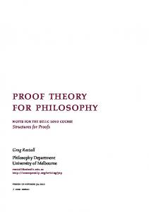
both unary as well as chopping modalities, our proof system is strongly related to both approaches. Besides providing a higher expressiveness, extending MLSL enables us to formulate and prove the invariance of the spatial safety property inside EMLSL and its deductive proof system. We demonstrate this by conducting a formal proof of the so called reservation lemma [HLOR11], which informally states that no car changes lanes without having set the turn signal beforehand. Further on, we show undecidability of a subset of EMLSL. We adapt the proof of Zhou et al. [ZHS93] for DC and reduce the halting problem of two counter machines to satisfiability of EMLSL formulas. Due to the restricted set of predicates EMLSL provides, this is non-trivial. The contributions of this paper are as follows: • we extend MLSL with lengths measurements and dynamic modalities (Sect. 2); • we show the spatial fragment of EMLSL to be undecidable (Sect. 3); • we present a suited proof system and derive the reservation lemma (Sect. 4). The differences to our publication in the proceedings of the 10th International Colloquium on Theoretical Aspects of Computing (ICTAC) in 2013 [LH13] are: • we include the proofs for the preservation of sanity conditions of the spatial situations along the transitions (Sect. 2), the undecidability result (Sect. 3) and the soundness of the proof system (Sect. 4); • we show an additional formal proof within the proof system for a theorem showing the independence of length measurement from the width (i.e., the number of lanes currently perceivable by a car; see Lemma 4.7). This proof is straightforwardly adaptable to a proof for the reversed situation, i.e., the independence of width measurement from the extension (the part of the highway currently perceived by a car in driving direction); • we added means of moving the part of the highway perceived by a car along the passing of time in Sect. 2. This addition has also impact on the form of the labelling algebra of the proof system in Sect. 4. 2. Extended MLSL Syntax and Semantics The purpose of EMLSL is to reason about highway situations. To this end, we first present the formal model of a traffic snapshot capturing the position and speed of every car on the highway at a given point in time. In addition a traffic snapshot comprises the lane a given car is driving on, which we call a reservation. Every car usually holds one reservation, i.e., drives on one lane, but may, during lane change maneuvers, hold up to two reservations on adjacent lanes. Furthermore, we capture the indication that a given car wants to change to a adjacent lane by the notion of a claim which is an abstraction of setting the turn signal. Every car may only hold claims while not engaged in a lane change. Intuitively, traffic snapshots shall formalize situations as depicted in Fig. 1. Each car drives at a certain horizontal position and reserves one or at most two lanes. The car E is currently claiming the lower lane, depicted by the dotted polygon. For a car, we subsume its physical size and its braking distance, i.e., the distance it needs to come to a safe standstill at its current speed, under its safety envelope. As an abstraction of sensor limitations, we assume each car to observe only a finite part of the road, called the view of the car. The dashed rectangle indicates a possible view of the car E.

PROOF THEORY OF A MULTI-LANE SPATIAL LOGIC

C

braking distance

3

safety envelope

physical size

E

A

B

E

A

Figure 1: Situation on a Motorway at a Single Point in Time To formally define a traffic snapshot, we assume a countably infinite set of globally unique car identifiers I and an arbitrary but fixed set of lanes L = {0, . . . , N }, for some N ≥ 1. Throughout this paper we will furthermore make use of the notation P(X) for the powerset of X, and the override notation ⊕ from Z for function updates [WD96], i.e., f ⊕ {x 7→ y}(z) = y if x = z and f (z) otherwise. Definition 2.1 (Traffic snapshot). A traffic snapshot T S = (res, clm, pos , spd , acc) is defined by the functions • res : I → P(L) such that res(C) is the set of lanes the car C reserves, • clm : I → P(L) such that clm(C) is the set of lanes the car C claims, • pos : I → R such that pos(C) is the position of the car C along the lanes, • spd : I → R such that spd (C) is the current speed of the car C, • acc : I → R such that acc(C) is the current acceleration of the car C. Furthermore, we require the following sanity conditions to hold for all C ∈ I. (1) res(C) ∩ clm(C) = ∅ (2) 1 ≤ |res(C)| ≤ 2 (3) 0 ≤ |clm(C)| ≤ 1 (4) 1 ≤ |res(C)| + |clm(C)| ≤ 2 (5) clm(C) 6= ∅ implies ∃n ∈ L • res(C) ∪ clm(C) = {n, n + 1} (6) |res(C)| = 2 or |clm(C)| = 1 holds only for finitely many C ∈ I. We denote the set of all traffic snapshots by TS. The kinds of transitions are twofold. First, we have discrete transitions defining the possibilities to create, mutate and remove claims and reservations. The other type of transitions handles abstractions of the dynamics of cars, i.e., they allow for instantaneous changes of accelerations and for the passing of time, during which the cars move according to a simple model of motion. For the results presented subsequently, we only require the changes of positions to be continuous. Definition 2.2 (Transitions). The following transitions describe the changes that may occur at a traffic snapshot T S = (res, clm, pos , spd , acc). c(C,n)

T S −−−−→T S ′

⇔

T S ′ = (res, clm′ , pos, spd , acc) ∧ |clm(C)| = 0 ∧ |res(C)| = 1

4

SVEN LINKER AND MARTIN HILSCHER

∧ res(C) ∩ {n + 1, n − 1} = 6 ∅ ∧ clm′ = clm ⊕ {C 7→ {n}} wd c(C)

T S −−−−−→T S ′

(2.1)

T S ′ = (res, clm′ , pos, spd , acc)

⇔

∧ clm′ = clm ⊕ {C 7→ ∅} r(C)

T S −−→T S ′

(2.2)

T S ′ = (res′ , clm′ , pos, spd , acc)

⇔

∧ clm′ = clm ⊕ {C 7→ ∅} ∧ res′ = res ⊕ {C 7→ res(C) ∪ clm(C)} wd r(C,n)

T S −−−−−−→T S ′

(2.3)

T S ′ = (res′ , clm, pos , spd , acc)

⇔

∧ res′ = res ⊕ {C 7→ {n}} ∧ n ∈ res(C) ∧ |res(C)| = 2 t

T S− →T S ′

(2.4)

T S ′ = (res, clm, pos ′ , spd ′ , acc)

⇔

∧ ∀C ∈ I : pos ′ (C) = pos(C) + spd (C) · t + 21 acc(C) · t2 ∧ ∀C ∈ I : spd ′ (C) = spd (C) + acc(C) · t acc(C,a)

T S −−−−−→T S ′

(2.5)

T S ′ = (res, clm, pos , spd , acc ′ )

⇔

∧ acc ′ = acc ⊕ {C 7→ a}

(2.6)

We also combine passing of time and changes of accelerations to evolutions. t

t

acc(C0 ,a0 )

t

acc(Cn ,an )

0 n TS ⇒ = T S ′ ⇔ T S = T S 0− →T S 1 −−−−−−→ . . . −→T S 2n−1 −−−−−−−→T S 2n = T S ′ , Pn where t = i=0 ti , ai ∈ R and Ci ∈ I for all 0 ≤ i ≤ n. The transitions preserve the sanity conditions in Def. 2.1.

Lemma 2.3 (Preservation of Sanity). Let T S be a snapshot satisfying the constraints given in Def. 2.1. Then, each structure T S ′ reachable by a transition is again a traffic snapshot satisfying Def. 2.1. Proof. We proceed by a case distinction. If the transition leading from T S to T S ′ is the passing of time, or the change of an acceleration, the constraints are still satisfied in T S ′ , since they only concern the amount and place of claims and reservations. wd c(C)

The removal of a claim T S −−−−−→T S ′ sets clm′ (C) = ∅. There are two possibilities. If clm(C) = ∅, then T S = T S ′ and hence satisfies the constraints trivially. Let clm(C) 6= ∅. After the transition, constraint 1 holds trivially, constraint 2 is not affected, constraint 3 holds, as does constraint 4. Constraint 5 holds trivially and satisfaction of constraint 6 follows since it is satisfied in T S and we only shrink the number of cars for which there exists a claim. c(C,n) Now let T S −−−−→T S ′ . Then by definition of the transition, res(C) on T S contains exactly one element, and clm(C) is empty. On T S ′ , clm′ (C) contains exactly n. Since {n + 1, n − 1} ∩ res(C) 6= ∅, n cannot be an element of res′ (C). Hence, the constraints 1 to 5 are satisfied. Since T S satisfied constraint 6, and only one car created a new claim, T S ′ still satisfies this constraint.

PROOF THEORY OF A MULTI-LANE SPATIAL LOGIC

5

wd r(C,n)

Consider T S −−−−−−→T S ′ . Since |res(C)| = 2, constraint 4 ensures that clm(C) = ∅, by which constraint 1, 3, 4 and 5 hold in T S ′ . Constraint 2 holds, since we overwrite res(C) with {n}. Constraint 6 holds by an argument similar to the withdrawal of a claim. r(C)

Finally, let T S −−→T S ′ . Again we have to consider two cases. First, if clm(C) = ∅, then T S = T S ′ , and hence the constraints hold. If clm(C) 6= ∅, we get by constraint 2 that clm(C) = {n} for some n ∈ L. By constraint 4, |res(C)| = 1, and by constraint 1, we get that after the transition |res(C)| = 2, i.e., constraint 2 holds. Constraint 1 and 5 hold now trivially. Constraint 3 holds since we reset clm′ (C) = ∅ and similarly for constraint 4. The number of cars with either two reservations or a claim is not changed, hence constraint 6 holds. Example 2.4. We formalize Fig. 1 as a traffic snapshot T S = (res, clm, pos , spd , acc). We will only present the subsets of the functions for the cars visible in the figure. Assuming that the set of lanes is L = {1, 2, 3}, where 1 denotes the lower lane and 3 the upper one, the functions defining the reservations and claims of T S are given by res(A) = {1, 2}

res(B) = {1}

res(C) = {3}

res(E) = {2}

clm(A) = ∅

clm(B) = ∅

clm(C) = ∅

clm(E) = {1}

For the function pos, we chose arbitrary real values which still satisfy the relative positions of the cars in the figure. Similarly, we instantiate the function spd such that the safety envelopes of the cars could match the figure. For example, since the safety envelope of B is larger than the safety envelope of C, B has to drive with a higher velocity. For simplicity, we assume that all cars are driving with constant velocity at the moment, i.e., for all cars, the function acc returns zero. pos(A) = 28

pos(B) = 3.5

pos(C) = 2

pos(E) = 14

spd (A) = 8

spd (B) = 14

spd (C) = 4

spd (E) = 11

This traffic snapshot satisfies the sanity conditions. c(E,n)

For no traffic snapshot T S ′ and lane n we have T S −−−−→T S ′ , since |clm(E)| = 6 0. wd r(B,n)

Similarly, there is no transition T S −−−−−−→T S ′ , since |res(B)| 6= 2. But, if we let T S ′ = (res′ , clm′ , pos , spd , acc) where res′ and clm′ coincide with their counterparts in T S except r(E)

for res′ (E) = {1, 2} and clm′ (E) = ∅, then T S −−→T S ′ . EMLSL restricts the parts of the motorway perceived by each car to so called views. Each view comprises a set of lanes and a real-valued interval, its length. Definition 2.5 (View). For a given traffic snapshot T S with a set of lanes L, a view V is defined as a structure V = (L, X, E), where • L = [l, n] ⊆ L is an interval of lanes that are visible in the view, • X = [r, t] ⊆ R is the extension that is visible in the view, • E ∈ I is the identifier of the car under consideration, the owner of the view. A subview of V is obtained by restricting the lanes and extension we observe. For this we ′ use sub- and superscript notation: V L = (L′ , X, E) and VX ′ = (L, X ′ , E), where L′ and X ′ are subintervals of L and X, respectively. While views define the range of the car’s sensors, we use a distinct function to model the capability of these sensors. That is, the perceived length of cars can be dependent on

6

SVEN LINKER AND MARTIN HILSCHER

the car under consideration. As an example, a car may calculate its own braking distance, while it can only perceive the physical size of all other cars. Definition 2.6 (Sensor Function). The car dependent sensor function ΩE : I × TS → R+ given a car identifier and a traffic snapshot provides the length of the corresponding car, as perceived by E. The intention of the sensor function is to parametrize the knowledge available to the cars and by that to easily allow for the consideration of different scenarios [HLOR11]. Remark 2.7 (Abbreviations). For a given view V = (L, X, E) and a traffic snapshot T S = (res, clm, pos, spd , acc) we use the following abbreviations: resV : I → P(L) with C 7→ res(C) ∩ L clmV : I → P(L) with C 7→ clm(C) ∩ L lenV : I → P(X) with C 7→ [pos(C), pos(C) + ΩE (C, T S)] ∩ X The functions resV and clmV are restrictions of their counterparts in T S to the sets of lanes considered in this view. The function lenV gives us the part of the view occupied by a car C.1 Example 2.8. To fully formalize Fig. 1, we have to a define a view V = (L, X, E) corresponding to the dashed rectangle. The set of lanes visible in V is L = {1, 2}. For the extension, we only have to choose values such that the relations of the figure are preserved, i.e., both E and A fit fully into the extension, the safety envelope of B is partially contained in X, while no part of C overlaps with it. Hence, we first have to define how the safety envelopes are perceived by E. ΩE (A, T S) = 10

ΩE (B, T S) = 11.5

ΩE (C, T S) = 7

ΩE (E, T S) = 13

Now we can choose, e.g., X = [12, 42]. With this view and sensor function, the derived functions of T S and V are as follows. resV (A) = {1, 2}

resV (B) = {1}

resV (C) = ∅

resV (E) = {2}

clmV (A) = ∅

clmV (B) = ∅

clmV (C) = ∅

clmV (E) = {1}

len V (A) = [28, 38]

len V (B) = [12, 15]

len V (C) = ∅

len V (E) = [14, 27]

Observe how the space occupied by B is reduced to fit into the view, and that the reservation of C is invisible for E, since the view only comprises both lower lanes. In the logic, the view shall be interpreted relatively to the owner of the view. If a t traffic snapshot T S evolves to T S ′ in the time t, i.e. T S = ⇒ T S ′ , the extension X of a view V = (L, X, E) has to be shifted by the difference of the positions of E in T S and T S ′ . For this purpose, we introduce the function mv , which given two snapshots T S, T S ′ and a view V computes the view V ′ corresponding to V after moving from T S to T S ′ . 1This presentation differs slightly from the first presentation of MLSL in two ways. First, we do not restrict the set of identifiers anymore to the cars “visible” to E. Since the functions for the reservations, claims or length return the empty set for cars outside of V , such cars cannot satisfy the corresponding atomic formulas. The definition of resV and clmV was altered due to a technical mistake in the previous form.

PROOF THEORY OF A MULTI-LANE SPATIAL LOGIC

7

Definition 2.9 (Moving a View). For two traffic snapshots T S = (res, clm, pos , spd , acc) and T S ′ = (res′ , clm′ , pos ′ , spd ′ , acc ′ ) and a view V = (L, [r, s], E), the result of moving V ′ from T S to T S ′ is given by mv TT SS (V ) = (L, [r + x, s + x], E), where x = pos ′ (E) − pos(E). Definition 2.10 formalizes the partitioning of discrete intervals. We need this slightly intricate notion to have a clearly defined chopping operation, even on the empty set of lanes. We want the empty set to be a valid interval of lanes, so that the smallest intervals of lanes and horizontal space behave similarly. Definition 2.10 (Chopping discrete intervals). Let I be a discrete interval, i.e., I = [l, n] for some l, n ∈ L or I = ∅. Then I = I 1 ⊖ I 2 if and only if I 1 ∪ I 2 = I, I 1 ∩ I 2 = ∅, and both I 1 and I 2 are discrete convex intervals, which implies max(I 1 ) + 1 = min(I 2 ) or I 1 = ∅ or I 2 = ∅. We define the following relations on views to have a consistent description of vertical and horizontal chopping operations. Definition 2.11 (Relations of Views). Let V1 , V2 and V be views of a snapshot T S. Then V = V1 ⊖V2 if and only if V = (L, X, E), L = L1 ⊖L2 , V1 = V L1 and V2 = V L2 . Furthermore, V = V1 ȅ V2 if and only if V = (L, [r, t], E) and there is an s ∈ [r, t] such that V1 = V[r,s] and V2 = V[s,t] . To abstract from the borders of real-valued intervals during the definition of the semantics, we define the following norm giving the length of such intervals. This notion coincides with the length measurement of DC [ZHR91]. We also define the cardinality of discrete intervals to be their length. Definition 2.12 (Measures of intervals). Let IR = [r, t] be a real-valued interval, i.e. r, t ∈ R. The measure of IR is the norm kIR k = t − r. For a discrete interval ID , the measure of ID is simply its cardinality |ID |. With the definition of measures, we can give the reason for the need of Def. 2.10. The smallest intervals in horizontal direction are point-intervals, e.g. I = [r, r] for some r ∈ R. The measure of I is kIk = 0. In contrast, if the smallest intervals of lanes were also pointintervals, i.e., sets of the form {n}, their measure would be |{n}| = 1. However, with the the empty set as the smallest interval of lanes, the measures behave similarly for both directions. We employ three sorts of variables. The set of variables ranging over car identifiers is denoted by CVar, with typical elements c and d. For referring to lengths and quantities of lanes, we use the sorts RVar and LVar ranging over real numbers and elements of the set of lanes L, respectively. The set of all variables is denoted by Var. To refer to the car owning the current view, we use the special constant ego. Furthermore we use the syntax ℓ for the length of a view, i.e., the length of the extension of the view and ω for the width, i.e., the number of lanes. For simplicity, we only allow for addition between correctly sorted terms. However, it is straightforward to augment the definition with further arithmetic operations.

8

SVEN LINKER AND MARTIN HILSCHER

Definition 2.13 (Syntax). We use the following definition of terms. θ ::= n | r | ego | u | ℓ | ω | θ1 + θ2 , where n ∈ L, r ∈ R and u ∈ Var and θi are both of the same sort, and not elements of CVar ∪ {ego}. We denote the set of terms with Θ. The syntax of the extended multi-lane spatial logic EMLSL is given as follows. φ ::= ⊥ | θ1 = θ2 | re(c) | cl (c) | φ1 → φ2 | ∀z • φ1 | φ1 a φ2 |

φ2 | Mφ φ1

where M ∈ {r(c) , c(c) , wd c(c) , wd r(c) , τ }, c ∈ CVar ∪ {ego}, z ∈ Var, and θ1 , θ2 ∈ Θ are of the same sort. We denote the set of all EMLSL formulas by Φ. Definition 2.14 (Valuation and Modification). A valuation is a function ν : Var ∪ {ego} → I ∪ R ∪ L. We silently assume valuations and their modifications to respect the sorts of variables. For a view V = (L, X, E), we lift ν to a function νV evaluating terms, where variables and ego are interpreted as in ν, and νV (ℓ) = kXk and νV (ω) = |L|. The function + is interpreted as addition. Definition 2.15 (Semantics). In the following, let θi be terms of the same sort, c ∈ CVar ∪ {ego} and z ∈ Var. The satisfaction of formulas with respect to a traffic snapshot T S, a view V = (L, X, E) and a valuation ν with ν(ego) = E is defined inductively as follows: T S, V, ν 6|= ⊥

for all T S, V, ν

T S, V, ν |= θ1 = θ2

⇔ νV (θ1 ) = νV (θ2 )

T S, V, ν |= re(c)

⇔ |L| = 1 and kXk > 0 and resV (ν(c)) = L and X = lenV (ν(c))

T S, V, ν |= cl(c)

⇔ |L| = 1 and kXk > 0 and clmV (ν(c)) = L and X = len V (ν(c))

T S, V, ν |= φ1 → φ2

⇔ T S, V, ν |= φ1 implies T S, V, ν |= φ2

T S, V, ν |= ∀z • φ

⇔ ∀ α ∈ I ∪ R ∪ L • T S, V, ν ⊕ {z 7→ α} |= φ

T S, V, ν |= φ1 a φ2

⇔ ∃V1 , V2 • V = V1 ȅ V2 and T S, V1 , ν |= φ1 and T S, V2 , ν |= φ2

T S, V, ν |=

φ2 φ1

⇔ ∃V1 , V2 • V = V1 ⊖ V2 and T S, V1 , ν |= φ1 and T S, V2 , ν |= φ2 r(ν(c))

T S, V, ν |= r(c) φ

⇔ ∀T S ′ • T S −−−−→T S ′ implies T S ′ , V, ν |= φ

T S, V, ν |= c(c) φ

⇔ ∀T S ′ , n • T S −−−−−→T S ′ implies T S ′ , V, ν |= φ

T S, V, ν |= wd

c(c) φ

⇔ ∀T S ′ • T S −−−−−−→T S ′ implies T S ′ , V, ν |= φ

T S, V, ν |= wd

r(c) φ

⇔ ∀T S ′ , n • T S −−−−−−−→T S ′ implies T S ′ , V, ν |= φ

T S, V, ν |= τ φ

c(ν(c),n)

wd c(ν(c))

wd r(ν(c),n) t

′

⇔ ∀T S ′ , t • T S = ⇒ T S ′ implies T S ′ , mv TT SS (V ), ν |= φ

PROOF THEORY OF A MULTI-LANE SPATIAL LOGIC

9

Observe that views are only moved whenever time passes between snapshots. In addition to the standard abbreviations of the remaining Boolean operators and the existential quantifier, we use ⊤ ≡ ¬⊥. An important derived modality of our previous work [HLOR11] is the somewhere modality   ⊤ hφi ≡ ⊤ a  φ  a ⊤. ⊤

Further, we use its dual operator everywhere. We abbreviate the modality somewhere along the extension of the view with the operator ♦ℓ , similar to the on some subinterval modality of DC. [φ] ≡ ¬ h¬φi

♦ℓ φ ≡ ⊤ a φ a ⊤

ℓ φ ≡ ¬♦ℓ ¬φ

Likewise, abbreviations can be defined to express the modality on some lane. Furthermore, we define the diamond modalities for the transitions as usual, i.e., ♦∗ φ ≡ ¬∗ ¬φ, where ∗ ∈ {r(c), c(c), wd r(c), wd c(c), τ }. In the first definition of MLSL, we included the atom free to denote free space on the road, i.e., space which is neither occupied by a reservation nor by a claim. It was not possible to derive this atom from the others, since we were unable to express the existence of exactly one lane and a non-zero extension in the view. However, in the current presentation, free can be defined within EMLSL. Observe that a view of non-zero extension can be characterized by ℓ > 0 ≡ ¬(ℓ = 0). free ≡ ℓ > 0 ∧ ω = 1 ∧ ∀c • ℓ (¬cl(c) ∧ ¬re(c)) Furthermore, we can define ℓ < r ≡ ¬(ℓ = r a ⊤) and use the superscript ϕr to abbreviate the schema ϕ ∧ ℓ = r. For reasons of clarity, we will not always use this abbreviation and write out the formula instead, to emphasize the restriction. As an example, the following formula defines the behavior of a safe distance controller, i.e., as long as the car starts in a situation with free space in front of it, the formula demands that after an arbitrary time, there is still free space left.      ω=x ω=x ∀x, y • ♦ℓ  re(ego) a free  → τ ♦ℓ  re(ego) a free  ω=y ω=y

We have to relate the lane in both the antecedent and the conclusion by the atoms ω = x and ω = y respectively. If we simply used hre(ego) a freei, it would be possible for the reservations to be on different lanes, and hence, we would not ensure that free space is in front of each of ego’s reservations at every point in time. However, the formula does not constrain how the situations may change, whenever reservations or claims are created or withdrawn. Observe that it is crucial to combine acceleration and time transitions into a single modality τ . Let ego drive on lane m with a velocity of v. If we only allowed for the passing of time, this formula would require all cars on m in front of ego to have a velocity vf ≥ v, while all cars behind ego had to drive with vb ≤ v. Hence the evolutions allow for more complex behavior in the underlying model. Like for ITL [Mos85] or DC [ZHR91], we call a formula flexible whenever its satisfaction is dependent on the current traffic snapshot and view. Otherwise the formula is rigid. However, since the spatial dimensions of EMLSL are not directly interrelated, we also

10

SVEN LINKER AND MARTIN HILSCHER

distinguish horizontally rigid and vertically rigid formulas. The satisfaction of the former is independent of the extension of views, while for the latter, the amount of lanes in a view is of no influence. If a formula is only independent of the current traffic snapshot, we call it dynamically rigid. Definition 2.16 (Types of Rigidity). Let φ be a formula of EMLSL. We call φ dynamically rigid, if it does not contain any spatial atom, i.e., re(c) or cl(c) as a subformula. Furthermore, we call φ horizontally rigid, if it is dynamically rigid and in addition does not contain ℓ as a term. Similarly, φ is vertically rigid, if it is dynamically rigid and does not contain ω as a term. If φ is both vertically and horizontally rigid, it is simply rigid. Lemma 2.17. Let φ by dynamically rigid and φH (φV ) be horizontally (vertically) rigid. Then for all traffic snapshots T S, T S ′ , views V , V1 , V2 and valuations ν, (1) T S, V, ν |= φ iff T S ′ , V, ν |= φ (2) Let V = V1 ȅ V2 . Then T S, V, ν |= φH iff T S, Vi , ν |= φH (for i ∈ {1, 2}). (3) Let V = V1 ⊖ V2 . Then T S, V, ν |= φV iff T S, Vi , ν |= φV (for i ∈ {1, 2}). Proof. By induction on the structure of EMLSL formulas. 3. Undecidability of pure MLSL In this section we give an undecidability result for the spatial fragment of EMLSL, i.e., we do not need the modalities for the discrete state changes of the model or the evolutions. We will call this fragment spatial MLSL, subsequently. We reduce the halting problem of two-counter machines, which is known to be undecidable [Min67], to satisfaction of spatial MLSL formulas. Intuitively, a two counter machine executes a branching program which manipulates a (control) state and increments and decrements two different counters c1 and c2 . Formally, two counter machines consist of a set of states Q = {q0 , . . . , qm }, distinguished initial and final states q0 , qfin ∈ Q and a set of instructions I of the form shown in Tab. 1 (the instructions for the counter c2 are analogous). The instructions mutate configurations of the form s = (qi , c1 , c2 ), where qi ∈ Q and c1 , c2 ∈ N into new configurations: Table 1: Instructions for counter c1 of a two-counter machine s Instruction s′ c+

1 q −→q j

(q, c1 , c2 )

c− 1

q −→qj , qn

(q, 0, c2 )

c− 1

(q, c + 1, c2 ) q −→qj , qn

(qj , c1 + 1, c2 ) (qj , 0, c2 ) (qn , c, c2 )

An run from the initial configuration of a two-counter machine (Q, q0 , qfin , I) is a sei

ip

0 quence of configurations (q0 , 0, 0)− → ...− →(qp+1 , cp+1 , c′p+1 ), where each ij is an instance of an instruction within I. If qp+1 = qfin , the run is halting. We follow the approach of Zhou et al. [ZHS93] for DC. They encode the configurations in recurring patterns of length 4k, where the first part constitutes the current state, followed by the contents of the first counter. The third part is filled with a marker to distinguish the

PROOF THEORY OF A MULTI-LANE SPATIAL LOGIC

11

counters, and is finally followed by the contents of the second counter. Each of these parts is exactly of length k. Zhou et al. could use distinct observables for the state of the machine, counters and separating delimiters, since DC allows for the definition of arbitrary many observable variables. We have to modify this encoding since within spatial MLSL we are restricted to two predicates for reservations and claims, and the derived predicate for free space, respectively. Furthermore, due to the constraints on EMLSL models in Def. 2.1, we cannot use multiple occurrences of reservations of a unique car to stand, e.g., for the values of one counter. Hence we have to existentially quantify all mentions of reservations and claims. We will never reach an upper limit of existing cars, since we assume I to be countably infinite. The current state of the machine qi is encoded by the number of lanes below the current configuration, the states of the counters is described by a sequence of reservations, separated by a single claim. To safely refer to the start of a configuration, we also use an additional marker consisting of a claim, an adjacent reservation and again a claim. Each part of the configurations is assumed to have length k. Free space separates the reservations within one counter from each other and from the delimiters. Intuitively, a configuration is encoded as follows: marker i 0

free, re

cl

.. .

.. .

free, re

cl

...

... .. .

...

... 5k

To enhance the readability of our encoding, we use the abbreviation marker ≡ ∃c • cl(c) a ∃c • re(c) a ∃c • cl(c) to denote the start of a configuration. Like Zhou et al., we ensure that reservations and claims are mutually exclusive. We do not have to consider free, since it is already defined as the absence of both reservations and claims. Observe that we use the square brackets to denote the everywhere modality (cf. Section 2). mutex = ∀c, d • [cl(c) → ¬re(d)) ∧ (re(c) → ¬cl(d)] . The initial marking (q0 , 0, 0) is then defined by the following formula.   [¬∃c • cl(c)] init =  marker k a free k a (∃c • cl (c))k a free k a (∃c • cl(c))k  a ⊤ ω=0

We have to ensure that the configurations occur periodically after every 5k spatial units. Therefore, we use the following schema Per (D). Observe that we only require that the lanes surrounding the formula D do not contain claims. This ensures on the one hand that no configuration lies in parallel with the formula D, since well-defined configurations have to include claims. On the other hand, it allows for satisfiability of the formula, since we do not forbid the occurrence of reservations, which are needed for the claims within the

12

SVEN LINKER AND MARTIN HILSCHER

configurations. 

[¬∃c • cl (c)] D Per (D) =  [¬∃c • cl (c)]





a ℓ = 5k → ℓ = 5k a

 [¬∃c • cl(c)]  D [¬∃c • cl(c)]

Note that we did not constrain on which lane the periodic behavior occurs. This will be defined by the encoding of the operations. Now we may define the periodicity of the delimiters and the counters. Here we also have to slightly deviate from Zhou et al.: we are not able to express the statement “almost everywhere free or re(c) holds,” directly. We have to encode it by ensuring that on every subinterval with a length greater than zero, we can find another subinterval which satisfies free or re(c). This expresses in particular, that no claim may occur, due to the mutual exclusion property. periodic = Per ((ℓ (ℓ > 0 → ⊤ a (free ∨ ∃c • re(c)) a ⊤) ∧ ω = 1)k ) ∧ Per((∃c • cl(c))k ) ∧ Per(marker k ) c+

1 We turn to the encoding of the operation qi −→ qj , i.e., the machine goes from qi to qj and increments the first counter by one. Similar to Zhou et al., we use encodings of the form ¬(D1 a ¬D2 ), meaning “whenever the beginning of the view satisfies D1 , the next part satisfies D2 .” The formula F1 copies the reservations of counter one of state qi to the corresponding places in counter one in state qj .   ⊤ F1 = ¬  marker k a ℓ < k a ∃c • re(c) a ((∃c • re(c) a ⊤) ∧ ℓ = 5k)  a ω=i   ⊤ ¬  ℓ = 0 ∨ (∃c • re(c) a ⊤)   ω=j

We use a similar formula Ff ree to copy the free space before the reservations. The formulas F2 and F3 handle the addition of another reservation to the counter. We have to distinguish between an empty counter and one already containing reservations.     ⊤ ⊤ F2 =  marker k a free k a ℓ = 5k  →  ⊤ a (free a ∃c • re(c) a free)k  ω=j ω=i   ⊤ F3 =  marker k a ℓ < k a ∃c • re(c) a ((free a ∃c • cl(c) a ⊤) ∧ ℓ = 6k)  → ω=i   ⊤  ⊤ a (free a ∃c • re(c) a free a ∃c • cl(c))k  ω=j

In addition, we need formulas which copy of contents of the second counter to the new configuration, similar to F1 .

PROOF THEORY OF A MULTI-LANE SPATIAL LOGIC

13

Let IC be the set of the machine’s instructions and F (i) be the conjunction of the formulas encoding operation i and qfin its final state. Then   ⊤ ^ halt (C) = init ∧ periodic ∧ mutex ∧ ℓ F (i) ∧ ♦ℓ  ∃c • cl (c)  . ω = fin i∈IC

If and only if halt (C) is satisfiable, the machine contains a halting run. This holds since only configurations may contain claims (as defined in the formalization of periodicity), and whenever the machine reaches its final state, it halts. Hence the halting problem of two counter machines with empty initial configuration reduces to satisfiability of spatial MLSL formulas. Proposition 3.1. Let C be a two counter machine. Then C has a halting run if and only if halt (C) is satisfiable. Proof. “if ”. Let T S, V, ν |= halt (C), where V = (L, X, E). Observe that all variables occurring in halt (C) are existentially quantified, and hence we may ignore the values of ν. We divide X into parts of length 5k, i.e., we have |X| = s · 5k + r, where 0 ≤ r < 5k, which means s [ [a + (d − 1) · 5k, a + d · 5k] ∪ [a + s · 5k, b]. X = [a, b] = d=1

Se

We denote d=1 [a + (d − 1) · 5k, a + d · 5k] by Xe . Let X ′ = [a + (d′ − 1) · 5k, a + d′ · 5k] and X ′′ = [a + d′ · 5k, a + (d′ + 1) · 5k] for some 0 < d′ < s. Now assume that at X ′ , lane m contains a configuration, i.e., {m}

T S, VX ′

|= marker k a (ℓ (ℓ > 0 → ⊤ a (free ∨ ∃c • re(c)) a ⊤) ∧ ω = 1)k a ∃c • cl(c)k a (ℓ (ℓ > 0 → ⊤ a (free ∨ ∃c • re(c)) a ⊤) ∧ ω = 1)k a ∃c • cl(c)k

By interpreting periodic on T S, VX ′ ∪X ′′ we get that there is a lane m′ such that {m′ }

T S, VX ′′

|= marker k a (ℓ (ℓ > 0 → ⊤ a (free ∨ ∃c • re(c)) a ⊤) ∧ ω = 1)k a ∃c • cl (c)k a (ℓ (ℓ > 0 → ⊤ a (free ∨ ∃c • re(c)) a ⊤) ∧ ω = 1)k a ∃c • cl (c)k

Furthermore, periodic prevents that there exists a lane different from m′ containing such a situation, since for it to hold, all other lanes are forbidden to contain claims at X ′′ . Hence we have exactly one configuration on all parts [a + (d − 1) · 5k, a + d · 5k]. We can extract a run for C from T S, V from halt (C) by induction on d as follows. Let d = 1. Then init ensures that on lane 0, there is a configuration with no reservations between marker and the first claim and between the first and the second claim. Hence, we have a run starting at and ending with (q0 , 0, 0). As the induction hypothesis, we assume that for 1 ≤ d < s, we can extract a run R = (q0 , 0, 0)− →∗ (qi , c1 , c2 ) from T S, VXd . For d + 1, we know by the arguments above, that there exists exactly one configuration on [a + d · 5k, a + (d + 1) · 5k]. Since C is deterministic,

14

SVEN LINKER AND MARTIN HILSCHER

for the configuration on lane i, there is at most one set of formulas applicable. We only show the case for instruction incrementing counter one. Let F1 , F2 , F3 , Ffree be the applicable formulas, which we will interpret on Xd+1 \ Xd−1 , i.e. the interval X+ = [a + (d − 1) · 5k, a + (d + 1) · 5k]. This interval is exactly 10k long and starts with marker k on lane i. Then F1 states that for each reservation in the representation of the first counter, i.e., where ℓ < k a ∃c • re(c) holds, we find a reservation on lane j exactly 5k space units onwards. The outermost negation ensures that each possible chop point is considered, in particular the chop points arbitrarly close to the end points of the reservations. Ffree ensures in a similar way, that for each free space in front of a reservation in this representation, we have free space exactly 5k space units onwards on lane j. Hence, all reservations and the free space in between is present on lane j. Now we consider two cases. When there is no reservation between the marker and the first single claim, then F2 replaces this free space by a reservation enclosed by free space, i.e., the end configuration of the run was (qi , 0, c2 ) and the resulting configuration is (qj , 1, c2 ). The second counter was copied like the first. If there was a reservation before the last free space, then F3 replaces this last free space similarly by a reservation enclosed by free space on lane j, i.e., the configuration (qi , c1 , c2 ) is changed to (qj , c1 + 1, c2 ). Hence, in both cases we defined the increment of counter 1 together with a state change from qi to qj , which is by construction an instruction of C, hence R− →(qj , c1 , c2 ) is a valid run of C. The other cases are analogous. Now if we did extract a run from the satisfying model of halt (C), we have two possibilities. First, if r = 0, then the configuration at step s is the last of R. Then the last conjunct of halt (C) ensures, that a final state was reached, hence R is a halting run. Otherwise, if r > 0, then similarly it is ensured that on this last part of V , the lane corresponding to the final state has been reached. Since also the last change has to be initiated by a formula as before, there is an instruction to complete R to a halting run. “only if ”. Let R = (q0 , 0, 0)− →∗ (qf in , c1 , c2 ) be a halting run of C with d + 1 configurations, i.e. qd = qf in . We create a model T S, V with V = (L, X, E) with |X| = (d + 1) · 5k and |L| = |Q| + 1 as follows. For a configuration (qi , c1 , c2 ) at step d′ , we define three cars Cd′ ,0 , Cd′ ,1 , Cd′ ,2 with pos(Cd′ ,e ) = d′ · 5k + e · k/3

for e ∈ {0, 1, 2}

res(Cd′ ,0 ) = res(Cd′ ,2 ) = {i + 1} res(Cd′ ,1 ) = {i} clm(Cd′ ,0 ) = clm(Cd′ ,2 ) = {i} ΩE (Cd′ ,e , T S) = k/3

for e ∈ {0, 1, 2}

k

These cars satisfy marker . For the claims marking the end of counter 1 and 2 respectively, we define Cd′ ,4 and Cd′ ,6 as follows. pos(Cd′ ,4 ) = d′ · 5k + 2k pos(Cd′ ,6 ) = d′ · 5k + 4k res(Cd′ ,4 ) = res(Cd′ ,6 ) = {i + 1} clm(Cd′ ,4 ) = clm(Cd′ ,6 ) = {i} ΩE (Cd′ ,4 , T S) = ΩE (Cd′ ,6 ) = k

PROOF THEORY OF A MULTI-LANE SPATIAL LOGIC

15

For the definition of the first counter, we need the maximum value max of both counters on the whole run. Then we define a sequence of cars Cd′ ,3,x , where 1 ≤ x ≤ c1 if c1 > 0. For each such car we set 

k pos(Cd′ ,3,x ) = d · 5k + 3k + (2x + 1) · 1 + 2 · max res(Cd′ ,3,x ) = {i} ′



clm(Cd′ ,3,x ) = ∅ k 1 + 2 · max Otherwise, no such sequence is added. For the second counter, we define a similar sequence Cd′ ,5,x with 1 ≤ x ≤ c2 if c2 > 0. If we create such sets of cars for each configuration, the formula halt (C) is satisfied, if the run is halting. ΩE (Cd′ ,3,x ) =

The main theorem of this section is a corollary of Prop. 3.1. Theorem 3.2. The satisfiability problem of spatial MLSL is undecidable. Even though we used the full power of spatial MLSL in the proof, i.e., we used both ℓ and ω, the proof would be possible without using the latter. For that, we would not be able to encode the state of the configuration in the lanes, but by a similar way to the markers in the formulas. For example, the formula (∃c • cl (c) a ∃c • re(c) a ∃c • cl(c))k would denote the state q0 , and with another iteration of re(c), it would denote q1 and so on. If we remove the references to more than one lane in each of the formulas above, the reservations and claims would already imply that only one lane exists, and hence, the use of ω within the abbreviation free could be omitted. This shows that spatial MLSL is already undecidable even if we only use ℓ. 4. Labelled Natural Deduction for EMLSL Despite the negative decidability result of the previous section, we define a system of labelled natural deduction [Gab96, BMV98, Vig00] for the full logic EMLSL. That is, the rules of the deduction system do not operate on formulas φ, but on labelled formulas w : φ, where w is a term of a labelling algebra and φ is a formula of EMLSL. They may connect the derivations of formulas and relations between the terms w to allow for a tighter relationship between both. The labelling algebra is more involved than for standard modal logics, since EMLSL is in essence a multi-dimensional logic, where the modalities are not interdefinable. Obviously, the spatial modalities can not be defined by the dynamic modalities and vice versa. Furthermore, neither can the dynamic modalities be defined by each other in general. Consider, e.g., the modalities r(c) and c(c) . Both of these modalities rely on different transitions between the models, which are only indirectly related. The labels of the algebra consist of tuples T S, V , where similar to the semantics, T S is the name of a traffic snapshot and V a view. The algebra is then twofold. The relations of the form V = V1 ȅV2 and V = V1 ⊖V2 define ternary reachability relations between views for the r(C)

spatial modalities. Relations between snapshots and views, e.g., T S, V −−→T S ′ , V describe the behavior of transitions. The relations within the labelling algebra for traffic snapshots

16

SVEN LINKER AND MARTIN HILSCHER

c(C)

directly correspond to the dynamic modalities. For example, we have T S, V −−−→T S ′ , V , c(C,n)

whenever there exists an n ∈ N such that T S −−−−→T S ′ . We do not give a deduction system for the transitions between snapshots, since the conditions needed to hold between them are of a very complex nature, i.e., they are definable only with the power of full first-order logic with functions, identity and arithmetic. Hence we would not achieve a system with a nice distinction between the relational deductions and the deductions of labelled formulas [BMV98, Vig00]. Furthermore, the possiblity of a transition may be dependent on properties of cars at any place within the traffic snapshot. This means that we would have to specify global dependencies, while all logical operations we have at hand are only able to denote local properties, i.e., properties of cars visible in the current view. Instead we simply assume the existence of the relations between snapshots whenever needed. That is, we will often have, e.g., the existence of a transition in our set of assumptions. This is sensible, since we often want to reason about the outcome of a specific transition (see, e.g., Lemma 4.6). However, we give simple rules defining that chopping of a view into two subviews is always possible. Definition 4.1 (Labelled Formulas and Relational Formulas). Let T S be a name for a traffic snapshot, V a name for a view and φ a formula according to Definition 2.13. Then T S, V : φ is a labelled formula of EMLSL. Furthermore, we use two types of relational α formulas. On the one hand, we use T S, V − →T S ′ , V ′ to denote the existence of a transition with the label α. On the other hand, the formulas V = V1 ȅ V2 and V = V1 ⊖ V2 describe that the view V can be horizontally (vertically, resp.) chopped into the views V1 and V2 . To have a meaningful soundness result of the calculus, we relate the semantics of labelled formulas with the semantics of normal formulas. Observe that we do not define a completely independent notion of models, but only use a valuation for this purpose. This is due to the semantic information which is still comprised within the views and traffic snapshots. Definition 4.2 (Satisfaction of Labelled Formulas). We say that a valuation ν satisfies a labelled formula T S, V : φ, written ν |= T S, V : φ if and only if T S, V, ν |= φ. Furthermore, r(c)

ν |= T S 1 , V −−→T S 2 , V wd r(c)

ν |= T S 1 , V −−−−→T S 2 , V c(c)

ν |= T S 1 , V −−→T S 2 , V wd c(c)

ν |= T S 1 , V −−−−→T S 2 , V τ

→ T S 2 , V2 ν |= T S 1 , V1 −

r(ν(c))

⇔ T S 1 −−−−→T S 2 , wd r(ν(c),n)

⇔ ∃n • T S 1 −−−−−−−→T S 2 , c(ν(c),n)

⇔ ∃n • T S 1 −−−−−→T S 2 wd c(ν(c))

⇔ T S 1 −−−−−−→T S 2 t

⇒ T S 2 and V2 = mv TT SS 21 (V1 ) ⇔ ∃t • T S 1 =

The relational formulas V = V1 ȅ V2 and V = V1 ⊖ V2 are independent of the valuation at hand, and hence are satisfied whenever V1 and V2 combined according to Definition 2.11 result in V .

PROOF THEORY OF A MULTI-LANE SPATIAL LOGIC

17

We lift the satisfaction relation also to sets of labelled formulas and relational formulas. Let ν be a valuation, Γ a set of labelled formulas and ∆ a set of relational formulas. Then ν |= ∆

⇔ ∀ρ ∈ ∆ • ν |= ρ

ν |= Γ

⇔ ∀ (T S, V : φ) ∈ Γ • ν |= T S, V : φ

ν |= (Γ, ∆)

⇔ ν |= Γ and ν |= ∆

Γ, ∆ |= T S, V : φ

⇔ ν |= (Γ, ∆) implies ν |= T S, V : φ for all valuations ν

Definition 4.3 (Derivation). A derivation of a labelled formula T S, V : φ from a set of labelled formulas Γ and a set of relational formulas ∆ is a tree, where the root is T S, V : φ, each leaf is an element of Γ or ∆ and each node within the tree is a result of an application of one of the rules defined subsequently. We denote the existence of such a derivation by Γ, ∆ ⊢ T S, V : φ. Following Rasmussen [Ras01], we define predicates for chop-freeness of formulas and rigidity of terms and formulas. To increase the deducible theorems, we differentiate between vertical and horizontal chop-freeness and rigidity. These properties are especially important for the correct instantiation of terms, i.e., for the elimination of universal quantifiers. Example 4.4. Consider the formula ∀x •



 ℓ=x →ℓ=x , ℓ=x

which is a theorem of MLSL, since the length of a view is not changed by chopping vertically. If we use classical universal quantifier instantiation and substitute the vertically flexible term ω for x, then we would get ℓ=ω → ℓ = ω. ℓ=ω

(4.1)

Now let V be a view satisfying the antecedent of (4.1). Then V can be vertically chopped such that its length equals its width on both subviews. Now let ℓ = c. Then also ω = c for both subviews. Since V consists of both these subviews, V satisfies ω = 2c. But the conclusion of (4.1) states that V should satisfy ω = ℓ = c. However, we could of course substitute x by the vertically rigid term ℓ. We denote vertical (horizontal) chop-freeness by the predicate vcf (hcf) and vertical (horizontal) rigidity by vri (hri). The rules for the definition of all four predicates are straightforward, since both rigidity and chop-freeness are syntactic properties. All atomic formulas are vertically and horizontally chop-free. For ⊘ being a Boolean operator or the horizontal chop a , the following rules give vertical chop-freeness. vcf(φ) vcf(ψ) vcf ⊘ I vcf(φ ⊘ ψ)

vcf(φ ⊘ ψ) vcf ⊘ E vcf(φ)

vcf(φ ⊘ ψ) vcf ⊘ E vcf(ψ)

The rules for quantifiers and the horizontal rules are defined similarly. For terms, ℓ is vertically rigid and ω is horizontally rigid. The spatial atoms re(c) and cl(c) are neither horizontally nor vertically rigid, since they require the view to possess an extension greater than zero and exactly one lane. Equality is both vertically and horizontally rigid, as long as both compared terms are rigid. We show some exemplary rules, where ⊗ is an arbitrary binary operator.

18

SVEN LINKER AND MARTIN HILSCHER

hri(φ ⊗ ψ) hri ⊗ E hri(φ)

hri(φ) hri(ψ) hri ⊗ I hri(φ ⊗ ψ)

hri(φ ⊗ ψ) hri ⊗ E hri(ψ)

We have only two simple rules for the relations between views. First, we state that each view V is decomposable into two subviews. This is true, since we allow for the empty view, i.e., the view without lanes or with a point-like extension. We use E to denote existential quantification over views. To use the relations between views, we have to be able to instantiate views, i.e., we have to introduce a rule for elimination of existential quantifiers over views. As a side condition for this elimination rule, we require that T S, V3 : φ is not dependent on any assumption including V1 or V2 as a label, except for V = V1 ⊖ V2 . The rule itself is a straightforward adaptation of the classical rule. Again, we only show the case for the vertical relations. EV ′ , V ′′ (V = V ′ ⊖ V ′′ )

VDec EV ′ , V ′′ (V = V ′ ⊖ V ′′ ) T S, V3 : φ

[V = V1 ⊖ V2 ] .. . T S, V3 : φ EE

The intuition of rigidity is formalized in the following rules. Whenever a formula is horizontally rigid, the formula holds on all views horizontally reachable from the current view. Observe that the traffic snapshot may change arbitrarily, since horizontally rigid formulas are also dynamically rigid. The rules for vertically rigidity are similar. T S, V : φ

hri(φ) V = V1 ȅ V2 RH T S ′ , V1 : φ

T S, V : φ

hri(φ) V = V1 ȅ V2 RH T S ′ , V2 : φ

T S, V1 : φ

hri(φ) V = V1 ȅ V2 RH ′ T S ,V : φ

T S, V2 : φ

hri(φ) V = V1 ȅ V2 RH ′ T S ,V : φ

For the first-order operators, we use the typical definitions of labelled natural deduction rules [BMV98]. The only difference lies in the rules for quantification. We may instantiate an universally quantified variable with a horizontally (vertically) rigid, if the formula is vertically (horizontally) chop-free. If the formula is completely chop-free, we may instantiate the variable with an arbitrary term. Similarly, rigid terms may instantiate x in arbitrary formulas. In all cases, a side condition for the instantiation is that s respects the sort of x. T S, V : ∀x • φ hcf(φ) T S, V : φ[x 7→ s]

vri(s)

∀E

T S, V : ∀x • φ hcf(φ) vcf(φ) ∀E T S, V : φ[x 7→ s]

T S, V : ∀x • φ vcf(φ) T S, V : φ[x 7→ s]

hri(s)

∀E

T S, V : ∀x • φ hri(s) vri(s) ∀E T S, V : φ[x 7→ s]

The elimination and introduction rules for the chop modalities are adopted from Rasmussen [Ras01], and resemble the rules for existential quantification. We only show the case for the horizontal chop, the rules for vertical chopping are obtained straightforwardly, by replacing horizontal modalities and relations by the vertical ones.

T S, V1 : φ

T S, V2 : ψ V = V1 ȅ V2 aI T S, V : φ a ψ

T S, V : φ a ψ

[T S, V1 : φ] [T S, V2 : ψ] [V = V1 ȅ V2 ] .. . T S′, V ′ : χ aE T S ′, V ′ : χ

PROOF THEORY OF A MULTI-LANE SPATIAL LOGIC

19

The chopping of intervals is not ambiguous, i.e., there is a unique view of a certain length at the beginning of a view. This is the single decomposition property [Dut95] of interval logics and captured in the following rules. Hence when there are two vertical chops of a view, and the upper parts are of equal width, we can derive that the same formulas hold on the lower parts. Even though we only show the vertical set of rules, similar rules hold for the horizontal chopping of views. T S, V1 : φ

T S, V2 : ω = s

T S, V2′ : ω = s T S, V1′ : φ

vri(s) V = V1 ⊖ V2

V = V1′ ⊖ V2′

T S, V2 : φ

T S, V1 : ω = s

T S, V1′ : ω = s T S, V2′ : φ

vri(s) V = V1 ⊖ V2

V = V1′ ⊖ V2′

VD

VD

The additivity of length and width can be formalized by the following rules. T S, V1 : ω = s

T S, V : ω = s + t

T S, V2 : ω = t vri(s) vri(t) V = V1 ⊖ V2 V +I T S, V : ω = s + t

vri(s) vri(t) T S ′, V ′ : φ

[T S, V1 : ω = s] [T S, V2 : ω = t] [V = V1 ⊖ V2 ] .. . T S ′, V ′ : φ V +E

The dynamic modalities are defined along the lines of Basin et al. [BMV98]. If a transition from the current snapshot is possible, the box modalities may be eliminated and if we can prove that under the assumption of a fresh transition α, φ holds on the now reachable snapshot, α φ holds. In the α introduction rule, the label T S ′ , V ′ may not α occur in any assumption T S ′ , V ′ : φ depends on, with the exception of T S, V − →T S ′ , V ′ . α

α

T S, V − →T S ′ , V ′ T S, V : α φ α E T S ′, V ′ : φ

[T S, V − →T S ′ , V ′ ] .. . T S ′, V ′ : φ  I T S, V : α φ α

Finally, we have to define how the spatial atoms behave with respect to occurring transitions. There are two types of rules in general, stability rules and activity rules. Stability rules define which atoms stay true after a snapshot changes according to a certain transition. The truth of all reservation and claims of cars not involved in the transition are unchanged. Only one stability rule for creating reservations includes the car which is the source of the transition. We will show this rule and one example for typical stability. The activity rules state how the reservations and claims of cars will change according to the transitions. The following stability rules show that whenever a car creates a new claim, the reservations and claims of other cars are unchanged. We have similar stability rules for the other types of transitions. T S, V : cl(c)

T S, V : re(c)

c(d)

T S, V −−→T S ′ , V T S ′ , V : cl (c) c(d)

T S, V −−→T S ′ , V T S ′ , V : re(c)

T S, V : c 6= d

c(c)

−−→S T S, V : c 6= d

c(c)

−−→S

20

SVEN LINKER AND MARTIN HILSCHER

The activity rule for c(c) implies two properties. First, a claim may only be created when only one reservation exists. Second, the newly created claim resides on one side of the existing reservation. Observe that we require the view under consideration to comprise both adjacent lanes of the reservation. If we dropped this assumption (i.e., removed the subformulas ω = 1), it would be possible for the newly created claim to reside outside of the view V , and hence the conclusion would not be satisfied. T S, V :

¬(re(c) ∨ cl(c)) ∧ ω = 1 re(c) ¬(re(c) ∨ cl(c)) ∧ ω = 1

c(d)

T S, V −−→T S ′ , V

T S, V : c = d c(c)

−−→A

cl (c) ¬(re(c) ∨ cl(c)) ∧ ω = 1 re(c) re(c) ∨ T S ′, V : ¬(re(c) ∨ cl(c)) ∧ ω = 1 cl(c)

Activity rules for the creation of reservations in between traffic snapshots are: T S, V : cl(c)

T S, V : re(c)

r(d)

T S, V −−→T S ′ , V T S ′ , V : re(c) r(d)

T S, V −−→T S ′ , V T S ′ , V : re(c)

T S, V : c = d

r(c)

−−→A1 T S, V : c = d

r(c)

−−→A2

The following activity rules define the withdrawal of reservations and claims. T S, V :

re(c) re(c)

wd r(d)

T S, V −−−−→T S ′ , V

T S, V : c = d

wd c(c)

wd r(c)

T S ′, V :

−−−−→A

¬re(c) re(c) ∨ re(c) ¬re(c)

T S, V −−−−→T S ′ , V wd c(c) −−−−→A T S ′ , V : ¬cl(c)

Note that we cannot define rules relating the spatial situations along evolutions of time. This is due to the fact that we lost all knowledge about the concrete dynamics of the underlying semantics. Hence all constraints of the cars’ behaviour have to be explicitly defined within EMLSL, like the exemplary requirement for a safe distance controller in Sect.2. We also have rules for “backwards” reasoning, i.e., if our current snapshot is reachable from another, we may draw conclusions about the originating snapshot. Again, we differentiate between activity and stability rules (omitted here). T S ′ , V : re(c)

r(d)

T S, V −−→T S ′ , V T S, V : re(c) ∨ cl(c) c(d)

T S ′ , V : cl (c)

T S ′, V :

ω=1 re(c) ω=1

T S, V −−→T S ′ , V T S, V : ¬cl(c) wd r(d)

T S, V −−−−→T S ′ , V

T S, V :

T S, V : c = d

r(c)

←−−A T S, V : c = d

c(c)

←−−A T S, V : c = d wd r(c)

re(c) re(c) ω=1

ω=1 ∨ re(c) re(c)

←−−−−A

Observe that we can not reason backwards along withdrawals of claims, since these may be taken anytime, even when no claim previously existed (cf. Def. 2.2).

PROOF THEORY OF A MULTI-LANE SPATIAL LOGIC

21

Theorem 4.5. The calculus of labelled natural deduction for EMLSL is sound. Proof. Since we do not have any inference rules for the transitions between snapshots and the rules for relations between views are straightforward, we only have to consider the case of derivations of labelled formulas. We proceed by induction on the length of derivations to show Γ, ∆ ⊢ T S, V : φ implies Γ, ∆ |= T S, V : φ. If T S, V : φ ∈ Γ, then trivially Γ, ∆ |= T S, V : φ. For the induction step, assume that for all smaller derivations Γi , ∆i ⊢ T S i , Vi : φi , we already have Γi , ∆i |= T S i , Vi : φi . We only show some exemplary cases, for the rigidity rules, the elimination of the universal quantifier. Proofs for the other rules are either analogous, or can be straightforwardly infered from the work of Rasmussen [Ras01], Basin et al. [BMV98] and Vigan`o [Vig00]. However, we explicitly prove the soundness of all activity rules for reasoning forwards and backwards along traffic transitions. The last step in the derivation is an application of RH . Then φ is horizontally rigid. Let Γ, ∆ ⊢ T S, V : φ, ∆′ = {V = V1 ȅ V2 } ∪ ∆ and ν |= (Γ, ∆′ ) and hence also ν |= (Γ, ∆). By the induction hypothesis, we have ν |= T S, V : φ. By Def. 4.2, we get T S, V, ν |= φ. Now we may use Lemma 2.17 twice, once to get T S ′ , V, ν |= φ (since φ is also dynamically rigid) and the second time to get T S ′ , V1 , ν |= φ. Finally, we have ν |= T S ′ , V1 : φ. The other cases of this rule are similarly proven. The last step in the derivation is an application of the first variant of ∀E. Then φ is horizontal chop free and s is vertically rigid. Let Γ, ∆ ⊢ T S, V : ∀x • φ and ν |= (Γ, ∆). By the induction hypothesis, we have ν |= T S, V : ∀x • φ, i.e., T S, V, ν |= ∀x • φ. Since φ is horizontal chop free, it may at most contain a vertical chop. However, the value νV (s) is constant on all vertical subviews of V , hence also for all subformulas of φ. All in all, T S, V, ν |= φ[x 7→ s], i.e., ν |= T S, V : φ[x 7→ s]. The other variants of the quantifier elimination are analogous. wd r(c)

The last step in the derivation is an application of −−−−→A. Then let Γ1 , ∆ ⊢ T S, V :

re(c) and Γ2 , ∆ ⊢ T S, V : c = d, re(c)

wd r(d)

with Γ1 ∪ Γ2 = Γ and T S, V −−−−→T S ′ , V ∈ ∆, which by the induction hypothesis implies both re(c) Γ1 , ∆ |= T S, V : and Γ2 , ∆ |= T S, V : c = d. re(c) We assume ν |= (Γ, ∆), i.e., ν |= (Γ1 , ∆) and ν |= (Γ2 , ∆). Hence ν |= T S, V :

wd r(d) re(c) , ν |= T S, V : c = d and ν |= T S, V −−−−→T S ′ , V. re(c)

Let V = V1 ⊖ V2 , such that T S, V1 , ν |= re(c) and T S, V2 , ν |= re(c) with Vi = (Li , Xi , E). wd r(ν(d),n0 )

We know that there is a n0 , such that T S −−−−−−−−→T S ′ . Let n0 ∈ L1 . Then by Definition 2.2, we have that res′V2 (ν(d)) = ∅, which means T S ′ , V2 , ν 6|= re(c), that is, T S ′ , V2 , ν |= ¬re(c). Furthermore, we have n0 ∈ res′V2 (ν(d)), i.e., T S ′ , V1 , ν |= re(c). By

22

SVEN LINKER AND MARTIN HILSCHER

definition of the vertical chop, we get T S ′ , V, ν |=

re(c) ¬re(c)

and hence T S ′ , V, ν |=

re(c) ¬re(c) ∨ . ¬re(c) re(c)

If n0 ∈ L2 , the reasoning is analogous. All in all, we get that ν |= T S ′ , V :

re(c) ¬re(c) ∨ . ¬re(c) re(c) r(c)

The last step in the derivation is an application of −−→A. Then let Γ1 , ∆ ⊢ T S, V : cl(c), r(d)

Γ2 , ∆ ⊢ T S, V : c = d, with Γ1 ∪ Γ2 = Γ and T S, V −−→T S ′ , V ∈ ∆. By the induction hypothesis we get Γ1 , ∆ |= T S, V : cl (c), Γ2 , ∆ |= T S, V : c = d. Now assume ν |= (Γ, ∆). r(ν(d))

That is, ν(c) = ν(d) and T S, V, ν |= cl(c) and T S −−−−→T S ′ . Thus clmV (ν(c)) = L, where L are the lanes of V . By Definition 2.2 we get that res′ (ν(d)) = res(ν(d)) ∪ clm(ν(d)) and, since ν(c) = ν(d), res′V (ν(c)) = clmV (ν(c)) = L. So T S ′ , V, ν |= re(c) and by that ν |= T S ′ , V : re(c). wd c(c)

Let the last step of the derivation be an application of −−−−→A. Furthermore, let wd c(c)

wd c(c)

wd c(ν(c))

Γ, ∆ ⊢ T S, V −−−−→T S ′ , V , i.e. T S, V −−−−→T S ′ , V ∈ ∆. Hence T S −−−−−−→T S ′ is true. That is, clm′ (ν(c)) = ∅ which implies T S ′ , V, ν |= ¬cl(c). Thus ν |= T S ′ , V : ¬cl(c). c(c)

Let the last step of the derivation be an application of −−→A. Furthermore we assume Γ1 , ∆ ⊢ T S, V :

¬(re(c) ∨ cl (c)) ∧ ω = 1 re(c) , ¬(re(c) ∨ cl (c)) ∧ ω = 1

c(d)

Γ2 , ∆ ⊢ T S, V : c = d and T S, V −−→T S ′ , V ∈ ∆. Furthermore, let Γ = Γ1 ∪ Γ2 and ν |= (Γ, ∆). That is, for V = (L, X, E), we know that L contains exactly three elements, say L = {n1 , n2 , n3 } and that res(ν(c)) = {n2 } and clm(ν(c)) = ∅. Now consider T S ′ . c(ν(d),n′ )

c(d)

Since ν |= T S, V −−→T S ′ , V , we have T S −−−−−−→T S ′ for either n′ = n1 or n′ = n3 . Furthermore, due to ν(c) = ν(d) we know that clm′ (ν(c)) = {n′ }. Say n′ = n1 . Then T S ′ , V {n1 } , ν |= cl(c). Note that the extension of V {n1 } has to be greater than zero, since the subview V {n2 } already satisfies re(c). Due to res = res′ , we get T S ′ , V ν |=

¬(re(c) ∨ cl (c)) ∧ ω = 1 re(c) cl (c)

⇒

¬(re(c) ∨ cl (c)) ∧ ω = 1 re(c) ν |= T S , V : cl (c)

⇒

ν |= T S ′ , V :

′

¬(re(c) ∨ cl (c)) ∧ ω = 1 re(c) ∨ cl (c)

The case where n′ = n3 is similar.

cl(c) re(c) . ¬(re(c) ∨ cl(c)) ∧ ω = 1

PROOF THEORY OF A MULTI-LANE SPATIAL LOGIC

23

c(c)

The last step of the derivation is an applicaton of ←−−A. Then Γ1 , ∆ ⊢ T S ′ , V : cl(c), wd r(d)

Γ2 , ∆ ⊢ T S, V : c = d, with Γ1 ∪ Γ2 = Γ and T S, V −−−−→T S ′ , V ∈ ∆, which by the induction hypothesis implies both Γ1 , ∆ |= T S ′ , V : cl (c) and Γ2 , ∆ |= T S, V : c = d. We assume ν |= (Γ1 , ∆) and ν |= (Γ2 , ∆). Since c = d is dynamically rigid, we also have ν |= T S ′ , V : c = d by Lemma 2.17. So νV (c) = νV (d). There can only be a transition creating a new claim for νV (c) from T S to T S ′ , if clm(νV (c)) = ∅ on T S. Hence, for each view V ′ , T S, V ′ , ν |= ¬cl(c). Hence in particular T S, V, ν |= ¬cl(c), i.e., ν |= T S, V : ¬cl(c). wd r(c)

Let the last step of the derivation be an application of ←−−−−A and let Γ1 , ∆ ⊢ T S ′ , V :

ω=1 wd r(d) re(c) , Γ2 , ∆ ⊢ T S ′ , V : c = d and T S, V −−−−→T S ′ ∈ ∆. ω=1

Now assume ν |= (Γ1 ∪ Γ2 , ∆). By the induction hypothesis, we get ν |= T S ′ , V :

ω=1 re(c) ω=1

and ν |= T S ′ , V : c = d.

By that we know that the set of lanes L of V = (L, X, E) contains exactly three elements, say L = {n1 , n2 , n3 } and by the semantics of the transitions (see Def. 2.2) and EMLSL (see Def. 2.15), we get res′ (ν(c)) = {n2 }. The transition exists only, when |res(ν(c))| = 2 and n2 ∈ res(ν(c)), so there are only two possibilities (due to the sanity conditions of Def. 2.1): n1 ∈ res(ν(c)) or n3 ∈ res(ν(c)). Say n1 ∈ res(ν(c)). Then T S, V, ν |=

ω=1 re(c) re(c)

and hence ν |= T S, V :

re(c) re(c) ω=1

∨

ω=1 re(c) . re(c)

The case for n3 ∈ res(ν(c)) is similar. r(c)

Let the last step in the derivation be an application of ←−−A and let furthermore r(d)

Γ1 , ∆ ⊢ T S ′ , V : re(c), Γ2 , ∆ ⊢ T S, V : c = d and T S, V −−→T S ′ , V ∈ ∆. By the induction hypothesis, we get Γ1 , ∆ |= T S ′ , V : re(c) and Γ2 , ∆ |= T S, V : c = d. Now let Γ = Γ1 ∪ Γ2 and ν |= (Γ, ∆). We then know that res′V (c) = {n} where V = (L, X, E) with L = {n} and kXk > 0. By Def. 2.2 and ν(c) = ν(d) we get that res′ (ν(c)) = res(ν(c)) ∪ clm(ν(c)). If n ∈ res(ν(c)), we have T S, V, ν |= re(c), which implies T S, V, ν |= re(c) ∨ cl(c). Similarly, if n ∈ clm(ν(c)), we get T S, V, ν |= cl(c), which implies T S, V, ν |= re(c) ∨ cl (c). That is, ν |= T S, V : re(c) ∨ cl (c). Since models of EMLSL are based on the real numbers, we cannot hope for a complete deduction system. Even if we used an infinite and dense field instead of the real numbers, it is in no way obvious, whether the resulting proof system would be complete. Typical approaches for constructing maximally consistent sets [Vig00] are not directly applicable, since they may result in an infinite number of lanes in the canonical model.

24

SVEN LINKER AND MARTIN HILSCHER

As an example, we derive a variant of the reservation lemma, which we proved informally in our previous work [HLOR11]. Lemma 4.6 (Reservation). A reservation of a car c observed directly after c created a reservation, was either already present or is due to a previously existing claim. I.e., assuming r(c)

T S, V −−→T S ′ , V , the formula (re(c) ∨ cl (c)) ↔ r(c) re(c) holds. Hence r(c)

{T S, V −−→T S ′ , V } ⊢ T S, V : (re(c) ∨ cl (c)) ↔ r(c) re(c). Proof. The existence of the transition is of major importance for the elimination of the box modality in the proof using the backwards reasoning rule. For reasons of simplicity, we use a variant of the stability rules and activity rules, where d in the transition has been replaced by c, and hence we do not need the extra assumption of T S, V : c = d. We use two auxiliary derivations ΠS and ΠA , which allow us to infer the existence of a reservation on the snapshot after taking a transition. r(c)

ΠS :

[T S, V : re(c)]1 [T S, V −−→T S ′ , V ]2 ′ T S , V : re(c)

ΠA :

[T S, V : cl(c)]1 [T S, V −−→T S ′ , V ]2 T S ′ , V : re(c)

r(c)

Derivation of ⊢ T S, V : (re(c) ∨ cl (c)) → r(c) re(c). ∨E1

ΠS

[T S, V : re(c) ∨ cl(c)]3 T S ′ , V : re(c) r(c) I2 T S, V : r(c) re(c)

ΠA

T S, V : (re(c) ∨ cl (c)) → r(c) re(c)

→ I3

r(c)

Derivation of {T S, V −−→T S ′ , V } ⊢ T S, V : r(c) re(c) → (re(c) ∨ cl(c)). [T S, V : r(c) re(c)]1

r(c)

T S, V −−→T S ′ , V

T S ′ , V : re(c)

r(c) E

r(c)

T S, V −−→T S ′ , V

T S, V : re(c) ∨ cl(c) → I1 T S, V : r(c) re(c) → (re(c) ∨ cl(c))

r(c)

←−−

A second example showing how the rigidity rules and chopping rules interact is the following. Lemma 4.7 (Independence of Length and Width). For all traffic snapshots and views, the length of the view is the same on all vertical subviews, i.e. T S, V :

ℓ=x ↔ ℓ = x. ℓ=x

ℓ=x → ℓ = x. We define two auxiliary subderivations, ℓ=x which are in essence applications of the rules for rigidity. Proof. First we show ⊢ T S, V :

ΠR i :

vri(ℓ) vri(x) vri(ℓ = x) RV

[V = V1 ⊖ V2 ]1 T S, V : ℓ = x

[T S, Vi : ℓ = x]1

PROOF THEORY OF A MULTI-LANE SPATIAL LOGIC

25

The eliminations of assumptions are due to the chop-elimination in the following proof. 

ℓ=x T S, V : ℓ=x



ΠR 1

2

ΠR 2

T S, V : ℓ = x → I2 ℓ=x →ℓ=x T S, V : ℓ=x

vCE1

Now we turn to the other direction. Here, we need to assume that the decomposition of the view into two subviews is possible, i.e., the derivation contains an application of the elimination rule for the existential quantifier for views. For reasons of readability, we define two subderivations ΠVi . In each of these derivations, we infer from the assumption, that V has an extension of length x, that also the subview Vi has an extension of length x. ΠVi :

vri(ℓ) vri(x) vri(ℓ = x)

[V = V1 ⊖ V2 ]2 T S, Vi : ℓ = x

[T S, V : ℓ = x]1

RV

The eliminations of the assumptions indicated by the indices are due to the rules used in the final derivation, as follows. ΠV2

ΠV1 EV ′ , V ′′ (V = V ′ ⊖ V ′′ ) T S, V :

ℓ=x ℓ=x

T S, V : ℓ = x →

[V = V1 ⊖ V2 ]2 vCI ℓ=x T S, V : ℓ=x EE2

ℓ=x ℓ=x

→ I1

By the combination of both these derivations and the usual shortcut for biimplication introduction, we get the desired result. 5. Related and Future Work Most related work on spatial logics is focused on purely qualitative spatial reasoning [vBB07], e.g., the expressible properties concern topological relations [RCC92]. Logics expressing quantitative spatial properties are rare, an example is Sch¨afer’s Shape Calculus (SC) [Sch05], which is a very general extension of DC. Contrasting SC, the focus of EMLSL lies on a restricted field of application, i.e., highway traffic. EMLSL is an instance of a multi-dimensional and multi-modal logic [GKWZ03], since it consists of various different modal operators, which are not interdefinable. However, the modalities are strongly interconnected, e.g. the creation of a reservation only has an effect, if there was a preceeding creation of a claim for the same car. Hence EMLSL is not simply a fusion of the corresponding uni-modal languages, but presumably determined by a class of suitable product frames. It is worthwile to study, which properties the parts of these frames are required to have. Labelled natural deduction for (multi-)modal logics has been studied intensely recently. E.g., when the rules for relational formulas can be defined with horn clauses as antecedents, nice meta-theoretical properties like normalization of proofs can be established [BMV98, Vig00]. In intuitionistic modal logic, similar results are obtained, when the relational theory

26

SVEN LINKER AND MARTIN HILSCHER

is defined using only geometric sequents [Sim94]. Unfortunately, even with our restricted set of rules for view relations, these results do not carry over to our setting, since we made use of existential quantification on views. Consider, e.g., the proof of Lemma 4.7. There the relational rule for the elimination of existential quantification over views is used within an otherwise purely logical deduction. Still we would like to explore how rules for the manipulation of traffic snapshots could blend in. However, due to the complex internal structure of traffic snapshots, we do not expect such rules to be definable by horn clauses. The labelling algebra is deeply intertwined with the predicates and operators of EMLSL. Changes in the former would induce adaptations in the latter and vice versa. For example, a possible extension would be to exchange the dynamical modality τ by a metric variant [a,b] , where a and b are elements of a suitable domain of time, say R. This change would τ have to be reflected in the labelling algebra by replacing the relation − → with transitions labelled by real numbers (or real-valued variables). Then rules expressing the properties of these relational formulas may be added, e.g., for additivity of durations. Rasga et al. investigated the fibring [CSS05] of labelled deductive systems [RSSV02]. We assume that the deduction system of Sec. 4 is an instance of such a fibring, where the Boolean operators are shared between all deduction systems involved. A further classification of EMLSL (or a suitable subset) and its proof system within the framework of fibring and multi-dimensional logics would be of interest in order to use preservation results concerning, e.g., decidability. To further increase the possible applications of EMLSL, we seek to introduce a global box modality . Intuitively, a formula φ shall express that φ is an invariant over all possible sequences of transitions. This modality is not expressible with the help of the other modalities and is intuitively similar to an iteration of the transitions like in dynamic logic [HTK00]. Finally, an implementation within a general theorem prover like Isabelle [Pau94] similar to implementations for modal or interval logics [BMV98, Vig00, Ras01] would increase the usefulness of the proof system. References [BMV98]

D. Basin, S. Matthews, and L. Vigan` o. Natural deduction for non-classical logics. Studia Logica, 60:119–160, 1998. [CSS05] C. Caleiro, A. Sernadas, and C. Sernadas. Fibring logics: Past, present and future. In We Will Show Them! Essays in Honour of Dov Gabbay, Volume 1, pages 363–388, 2005. [Dut95] B. Dutertre. Complete proof systems for first order interval temporal logic. In Symposium on Logic in Computer Science 1995, pages 36–43. IEEE Computer Society, 1995. [Gab96] D. M. Gabbay. Labelled deductive systems, volume 1. Oxford University Press, 1996. [GKWZ03] D. M. Gabbay, A. Kurucz, F. Wolter, and M. Zakharyaschev. Many-dimensional modal logics: theory and applications, volume 148 of Studies in Logic and the Foundations of Mathematics. Elsevier, 2003. [HLOR11] M. Hilscher, S. Linker, E.R. Olderog, and A. P. Ravn. An abstract model for proving safety of multi-lane traffic manoeuvres. In Int’l Conference on Formal Engineering Methods 2011, pages 404–419. Springer, 2011. [HTK00] D. Harel, J. Tiuryn, and D. Kozen. Dynamic Logic. MIT Press, Cambridge, MA, USA, 2000. [LH13] S. Linker and M. Hilscher. Proof theory of a multi-lane spatial logic. In Zhiming L., J. Woodcock, and Huibiao Z., editors, Int’l Colloquium on Theoretical Aspects of Computing 2013, pages 231– 248. Springer, 2013. [Min67] M. L. Minsky. Computation: finite and infinite machines. Prentice-Hall, Inc., 1967. [Mos85] B. Moszkowski. A temporal logic for multilevel reasoning about hardware. Computer, 18(2):10– 19, 1985.

PROOF THEORY OF A MULTI-LANE SPATIAL LOGIC

[Pau94] [Ras01] [RCC92] [RSSV02] [Sch05] [Sim94] [vBB07]

[Vig00] [WD96] [ZHR91] [ZHS93]

27

L. Paulson. Isabelle: A Generic Theorem Prover. Springer, 1994. T. M. Rasmussen. Labelled natural deduction for interval logics. In L. Fribourg, editor, CSL, pages 308–323. Springer, 2001. D. A. Randell, Z. Cui, and A. G. Cohn. A Spatial Logic based on Regions and Connection. In Int’l Conf. on Knowledge Representation and Reasoning 1992, 1992. J. Rasga, A. Sernadas, C. Sernadas, and L. Vigan` o. Fibring labelled deduction systems. Journal of Logic and Computation, 12(3):443–473, 2002. A. Sch¨ afer. A calculus for shapes in time and space. In Zhiming L. and K. Araki, editors, Int’l Colloquium on Theoretical Aspects of Computing 2004, pages 463–478. Springer, 2005. A. K. Simpson. The Proof Theory and Semantics of Intuitionistic Modal Logic. PhD thesis, University of Edinburgh, 1994. J. van Benthem and G. Bezhanishvili. Modal logics of space. In Marco Aiello, Ian PrattHartmann, and Johan Benthem, editors, Handbook of Spatial Logics, pages 217–298. Springer, 2007. L. Vigan` o. Labelled Non-Classical Logics. Kluwer Academic Publishers, 2000. J. Woodcock and J. Davies. Using Z – Specification, Refinement, and Proof. Prentice Hall, 1996. Zhou C., C. A. R. Hoare, and A. P. Ravn. A calculus of durations. Information Processing Letters, 40(5):269 – 276, 1991. Zhou C., M. R. Hansen, and P. Sestoft. Decidability and undecidability results for duration calculus. In P. Enjalbert, A. Finkel, and K.W. Wagner, editors, Symposium on Theoretical Aspects of Computer Science 1993, pages 58–68. Springer, 1993.

This work is licensed under the Creative Commons Attribution-NoDerivs License. To view a copy of this license, visit http://creativecommons.org/licenses/by-nd/2.0/ or send a letter to Creative Commons, 171 Second St, Suite 300, San Francisco, CA 94105, USA, or Eisenacher Strasse 2, 10777 Berlin, Germany