PHYSICAL REVIEW B 68, 045415 共2003兲
Propagation of light in metallic nanowire arrays: Finite-difference time-domain studies of silver cylinders Stephen K. Gray* and Teobald Kupka Chemistry Division, Argonne National Laboratory, Argonne, Illinois 60439, USA 共Received 6 January 2003; published 16 July 2003兲 Finite-difference time-domain studies of a variety of silver cylinder arrays with nanometer-scale diameters 共nanowires兲 interacting with light are presented. We show how reasonable estimates of scattering and absorption cross sections for metallic nanoscale objects can be obtained from such calculations. We then study the explicit time-domain behavior of both simple linear chains of such cylinders, as well as more elaborate arrays. A funnel-like configuration is found to be one interesting possibility for achieving propagation of light through features confined in one dimension to less than 100 nm. DOI: 10.1103/PhysRevB.68.045415
PACS number共s兲: 78.67.⫺n, 42.25.Fx, 42.79.Gn, 73.20.Mf
I. INTRODUCTION
The absorption and scattering of light by small particles, including metal nanoparticles 共MNP’s兲, is an old and extensively studied subject.1 Nonetheless modern experimental methods, including near-field scanning optical microscopy2 共NSOM兲 and nanolithography,3 coupled with the desire to develop nanophotonics and nanoelectronics applications, have brought this venerable area to the forefront of current scientific research. Here we show how finite-difference time-domain4 – 6 FDTD calculations can be used to study light interacting with arrays of silver cylinders with nanoscale diameters, and we carry out a variety of studies of various configurations. The cylinders can be viewed as metallic nanowires and exhibit optical behavior similar to MNP’s. In particular, surface plasmon polaritons 共SPP’s兲, resonance interactions of light with electronic charge density near the metal surface,7 can play an important role. Motivation for our work comes from earlier theoretical work suggesting that coupled SPP’s in arrays of MNP’s could be used to confine and guide light at the subdiffraction limit.8 –10 In a related development, SPPmediated subdiffraction limit transport of light in gold nanowires has recently been demonstrated.11 Additional motivation for our work is provided by recent work of Wurtz and co-workers using NSOM techniques to explore a variety of aspects of silver nanoparticles,12–14 as well as ultrafast spectroscopic work of Scherer and co-workers.15,16 Since Quinten et al.8 suggested the possibility of propagating light in chains of MNP’s, a number of other theoretical studies have appeared. Most of this work is based on frequency-domain solutions to Maxwell’s equations. The interesting theoretical studies of Kottmann, Martin, and co-workers17–19 and Stockman, Faleev, and Bergman20,21 are particularly relevant to our work. Actually, the electrodynamics of MNP’s and nanoparticle clusters has also been of interest in physical chemistry for some time now, owing to the phenomenon of surface-enhanced Raman spectroscopy 共SERS兲.22 Kelly and co-workers have carried out a variety of theoretical studies of MNP clusters23–27 of relevance to SERS and also to biosensors. The theoretical approach adopted here, a time-domain one, is complementary to the 0163-1829/2003/68共4兲/045415共11兲/$20.00
work noted above. It is also very general and can be adapted to a variety of problems. See also the important related work of Maier, Kik, and Atwater,10 who recently presented FDTD results pertaining to a collective surface-plasmon resonance in linear arrays of gold spheres. Section II outlines our theoretical and computational methods. Section III presents cross-section results for linear chains, and Sec. IV presents time-evolution studies of various cylinder arrays. A funnel-like configuration is shown to have some promise for achieving propagation of light through sub-100 nm features. Section V concludes the paper and the Appendix discusses our modeling of the dielectric constant. II. THEORETICAL METHODS
The systems of interest to us are lossy and dispersive, so that special care must be taken in designing an appropriate FDTD 共Refs. 4 – 6兲 approach. We outline here the approach we have found to be useful. A. FDTD scheme in the presence of metal nanoparticles
Frequency-domain solutions to Maxwell’s equations for light interacting with materials are constructed by allowing spatial (x,y,z) and possibly light frequency 共兲 variation in the dielectric constant . In a region of space 兵 x,y,z 其 occupied by a metal, can be complex valued and frequency dependent: ⫽ o 关 r ( )⫹i i ( ) 兴 . A positive imaginary part i is associated with absorption and a negative real part r with reflection. Difficulties arise in attempting to construct time-domain solutions to Maxwell’s equations via the FDTD method in this case. The inclusion of frequency dependence 共dispersion兲 in is one issue. A more pragmatic problem is that negative r values make the standard time iteration scheme unstable. One alternative is to introduce currentdensity terms into Maxwell’s equation that are formally equivalent 共upon Fourier transformation to the frequency domain兲 to the use of a complex-valued, frequency-dependent dielectric constant.5,28 –31 For example, we adopt the following limiting case for Maxwell’s equations,
1 E共 x,y,z,t 兲 ⫽ 关 ⵜ⫻H共 x,y,z,t 兲 ⫺J共 x,y,z,t 兲兴 , t eff共 x,y,z 兲
68 045415-1
©2003 The American Physical Society
PHYSICAL REVIEW B 68, 045415 共2003兲
STEPHEN K. GRAY AND TEOBALD KUPKA
1 H共 x,y,z,t 兲 ⫽⫺ ⵜ⫻E共 x,y,z,t 兲 , t o J共 x,y,z,t 兲 ⫽ ␣ 共 x,y,z 兲 J共 x,y,z,t 兲 ⫹  共 x,y,z 兲 E共 x,y,z,t 兲 . t 共2.1兲 In regions of free space, or some dielectric material with a positive, real dielectric constant, ␣ ⫽  ⫽0, and if the current-density vector J is initially zero in these regions, it remains zero. In free space, eff⫽o . In metallic regions, eff , ␣, and  take on values characteristic of the metal. Equation 共2.1兲 is consistent with the real and imaginary parts of a standard Drude model1 for the dielectric constant of a metal. However, as outlined in the Appendix, we can numerically fit a Drude model to empirical dielectric constant behavior in any localized region of frequency space, achieving a reasonably accurate modeling of any frequency region. 共See Refs. 5, 28, and 29 for other approaches.兲 The three parameters of the Drude model 共see the Appendix兲 are r (⬁), D , and ⌫ D . In a metallic region we then use eff⫽ o r 共 ⬁ 兲 ,
␣ ⫽⫺⌫ D ,  ⫽ o D2
共2.2兲
in Eq. 共2.1兲. Specializing to the transverse electric 共TE兲 case with cylindrical symmetry, we drop the z coordinate in all equations and deal with just three of the six field components, E x , E y , and H z (E z ⫽H x ⫽H y ⫽0). With discrete time steps , and (x,y)⬅E x 关 x,y,t⫽(n⫹1/2) 兴 , etc., for n notation E n⫹1/2 x ⫽0, 1,..., the FDTD propagation scheme is
冋 冋
册 册 册
E n⫹1/2 共 x,y 兲 ⫽E n⫺1/2 共 x,y 兲 ⫹ x x
H zn n ⫺J x , eff共 x,y 兲 y
E n⫹1/2 共 x,y 兲 ⫽E n⫺1/2 共 x,y 兲 ⫺ y y
H zn n ⫺J y , eff共 x,y 兲 x
H zn⫹1 共 x,y 兲 ⫽H zn 共 x,y 兲 ⫹
冋
E n⫹1/2 E n⫹1/2 y x ⫺ o x y
共2.3a兲
30
along with the current-density updates J n⫹1 共 x,y 兲 ⫽ x
冋
⫹ J n⫹1 共 x,y 兲 ⫽ y
冋
册
1⫹ ␣ 共 x,y 兲 /2 n J 共 x,y 兲 1⫺ ␣ 共 x,y 兲 /2 x
冋
册
 共 x,y 兲 E n⫹1/2共 x,y 兲 , 1⫺ ␣ 共 x,y 兲 /2 x
册
1⫹ ␣ 共 x,y 兲 /2 n J 共 x,y 兲 1⫺ ␣ 共 x,y 兲 /2 y
⫹
冋
册
 共 x,y 兲 E n⫹1/2共 x,y 兲 . 1⫺ ␣ 共 x,y 兲 /2 y
In addition to the time leapfrogging in Eq. 共2.3兲, we follow the standard FDTD approach of employing evenly spaced but staggered spatial grids,4,5 i.e., the x and y grids for E x , E y , and H z are all slightly different, which leads to a particularly accurate evaluation of the relevant derivatives via simple two-point finite differences. Absorption of field components approaching the boundaries of the grid must be carried out in order to prevent spurious reflections. For each of the x and y grids, absorbing regions are set up in the initial and final portions of these grids and simple exponential damping of the electric and magnetic fields, as typically accomplished in quantum wavepacket work,32,33 is carried out after each time step. For example, if x min and x max denote the lower and upper values of x, we define left and right absorption strips in 关 x min,x L 兴 and 关 x R ,x max兴 . Each field component is then multiplied by exp关⫺s(x⫺xL)2兴 for x⬍x L and exp关⫺s(x⫺xR)2兴 for x⬎x R 共for all y兲. A similar absorption along the y absorption regions 共for all x兲 is also carried out. Typically, 20%–30% of our grids are devoted to absorption and a gentle strength s, such that, after each absorption, the field values are decreased by 0.9 at the grid edges. 共The time steps are typically very small, which is why such a gentle absorption is effective.兲 A better absorption, also with the use of smaller absorbing boundaries, could probably be accomplished with the use of more sophisticated perfectly matched layer approaches.5,34 We employ two types of initial conditions. The simplest one is to specify at t⫽0 some specific pulse. For example, a Gaussian-damped sinusoidal pulse moving from left to right ⫽0 and in x with wave vector k O ⫽ O /c is given by E n⫽⫺1/2 x E n⫽⫺1/2 共 x,y 兲 ⫽g x 共 x 兲 g y 共 y 兲 cos共 k o x⫺ o /2兲 , y H zn⫽0 共 x,y 兲 ⫽g x 共 x 兲 g y 共 y 兲 cos共 k o x 兲 .
共2.4兲
The Gaussian functions g x and g y are then chosen such that the pulse has some desired central position and spatial extent. Owing to the finite extent, the pulse provides frequency content for a range of frequencies about o . Such initial conditions are well suited to computational experiments that probe directly the application of short pulses of light to arbitrary places in MNP array structures. Another type of initial condition we use is a plane-wave source located on a line in y for a fixed value of x. Typically, for some finite time period a plane wave moving forward in x emanates from such a line, with a fixed x value typically chosen to be just after the absorbing boundary in x. Since the wave emanates from a line, it is possible to achieve, effectively, a longer wave train and hence better frequency resolution 共if that is desired兲 than defining a full, long initial pulse on a given grid as above. We find that the scattered field/total field approach for achieving such a source 共see, e.g., Ref. 5, and references therein兲 is reliable and easy to implement. This approach is also somewhat more efficient for obtaining accurate frequency-domain results such as cross sections. B. Cross-section formulas
共2.3b兲
We use a simple, direct procedure, which is both feasible and sufficiently accurate for our purposes, to estimate cross
045415-2
PHYSICAL REVIEW B 68, 045415 共2003兲
PROPAGATION OF LIGHT IN METALLIC NANOWIRE . . .
sections 共Near- to far-field transformations5,6 could provide greater efficiency but we had no need to implement them in this study.兲 Given real-valued time-dependent electric- and magnetic-field vectors E(t)⬅E(x,y,z,t) and H(t) ⬅H(x,y,z,t), as determined in Sec. II A, consistent with an appropriate initial pulse or a source, and scattering off one or more particles, the complex, frequency-resolved total fields are E共 兲 ⫽ H共 兲 ⫽
冕 冕
⬁
0
with P abs共 兲 ⫽r ⬁
Hinc共 兲 ⫽
d S共 兲 •r兩 r⫽r ⬁ ,
dt exp共 i t 兲 E共 t 兲 , dt exp共 i t 兲 H共 t 兲 .
⬁
0 ⬁
0
共2.5兲
共2.13兲
A useful check of the numerical calculations is to determine the extinction cross section directly via the formula
ext共 兲 ⫽
P ext共 兲 , I inc共 兲
共2.14兲
where dt exp共 i t 兲 Einc共 t 兲 , dt exp共 i t 兲 Hinc共 t 兲 .
Esca共 兲 ⫽E共 兲 ⫺Einc共 兲 ,
P ext共 兲 ⫽r ⬁ 共2.6兲
Hsca共 兲 ⫽H共 兲 ⫺Hinc共 兲 . 共2.7兲
Following Bohren and Huffman,1 ‘‘cross sections’’ per unit length of the cylinder axis, which therefore have units of length as opposed to length,2 are calculated. The corresponding scattering cross section is
sca共 兲 ⫽
P sca共 兲 , I inc共 兲
共2.8兲
where P sca is the scattered power per unit length 共energy/ time/length兲 and I inc is the magnitude of the incident flux or power per unit area. In terms of the 共time-averaged兲 Poynting vector associated with the scattered fields, Ssca , and employing cylindrical coordinates (r, ,z),
冕
共2.12兲
The extinction cross section is the sum of the scattering and absorption cross sections,
共Analytical results could of course be used for the incident fields. However, a separate numerical calculation of the incident fields with the same grids and other features as for the total fields is more consistent, and will yield more accurate cross sections.兲 The scattered fields are then given by
P sca共 兲 ⫽r ⬁
0
ext共 兲 ⫽ sca共 兲 ⫹ abs共 兲 .
⬁
0
冕 冕
2
1 S共 兲 ⫽ Re关 E共 兲 ⫻H共 兲 * 兴 . 2
A comparable calculation, but in the absence of particles, yields incident time-dependent fields Einc(t) and Hinc(t), with the frequency-resolved incident fields Einc共 兲 ⫽
冕
2
0
d Ssca共 兲 •r兩 r⫽r ⬁ ,
共2.9兲
where the path of integration is along a circle of large radius r ⬁ surrounding the cylinder for any value of z, and 1 Ssca共 兲 ⫽ Re关 Esca共 兲 ⫻Hsca共 兲 * 兴 . 2
共2.10兲
The absorption cross section is given by
sca共 兲 ⫽
P abs共 兲 , I inc共 兲
共2.11兲
冕
2
0
d Sext共 兲 •r兩 r⫽r ⬁ ,
1 Sext共 兲 ⫽ Re关 Einc共 兲 ⫻Hsca共 兲 * ⫹Esca共 兲 ⫻Hinc共 兲 * 兴 . 2 共2.15兲 C. Numerical details
The two-dimensional nature of the problem allows us to employ large, dense grids without excessive computational burden. We generally consider grids in x and y ranging from ⫺1000 to 1000 nm, with the silver cylinder structures centered about the origin. Absorption, as discussed in Sec. II A, is carried out in the first and last 400 nm of each grid, allowing for a 1200⫻1200 nm interaction region. For cylinders with radii a⫽25 nm, even a coarse spatial grid spacings ⌬x⫽⌬y⫽⌬⫽2.7 nm 共750 grid points in each direction兲 yield reasonable results, although to assure good convergence we have actually used ⌬⫽1 nm 共2000 grid points in each direction兲 in all the results presented here. Given the current updated equations,30 time steps just under the Courant stability limit C ⫽⌬/(3 1/2c) yield stable solutions; however, for good convergence we chose to use steps ⫽ C /2. A given propagation is generally carried out up to times on the order of 0.15⫻10⫺13 s, which with our most dense (2000 ⫻2000) grid can require several hours of computation time on a 1-GHz Pentium III processor. 共However, calculations based on smaller grids of, say, 500⫻500 dimensions, can be qualitatively correct and require 10–20 min of computer time.兲 In estimating cross sections, we Fourier transform on field components along a circle about the origin with r ⬁ ⫽580 nm. 共Interestingly, almost identical results are obtained with radii as small as r ⬁ ⫽500 nm.) A typical source initial condition would correspond to a frequency o in the central portion of the wavelength region of interest, with the source placed just at the edge of the absorption region 共e.g., x⫽⫺600 nm) and turned on for the first 0.65⫻10⫺15 s.
045415-3
PHYSICAL REVIEW B 68, 045415 共2003兲
STEPHEN K. GRAY AND TEOBALD KUPKA
TABLE I. Drude parametrizations based on the Lynch-Hnter 共Ref. 36兲 refractive index compilation for silver.
FIG. 1. Cross sections for a single Ag cylinder of radius a ⫽25 nm. 共a兲 Scattering cross sections based on the Johnson-Christy 共Ref. 35兲 共open circles兲 and Lynch-Hunter 共Ref. 36兲 共filled circles兲 dielectric constant data. 共b兲 Scattering, absorption, and extinction cross sections calculated with Drude fit D1 of Table I 共smooth curves兲. 共c兲 Cross sections calculated with Drude fit D2 of Table I 共smooth curves兲. In 共b兲 and 共c兲 the symbols represent the cross sections calculated with the explicit dielectric constant data from Lynch and Hunter 共Ref. 36兲.
Set
D 共⬁兲
D 共eV兲
⌫ D 共eV兲
D1 D2
8.926 5.976
11.585 9.812
0.203 0.259
electric constant data. The open circles are cross sections inferred from the commonly used Johnson and Christy refractive index data set,35 and the filled circles are cross sections inferred from a somewhat more recent compilation of experimental results by Lynch and Hunter.36 It is interesting to note the sensitivity of the cross sections to the underlying dielectric constant data and this should serve as a cautionary note regarding quantitative prediction. We chose to base our calculations on the data compiled by Lynch and Hunter.36 As discussed in the Appendix, we fit Drude models to the empirically inferred dielectric constant data. Table I presents two such parametrizations of the Lynch and Hunter36 compilation, focusing on data in the ⫽(2 c/ ) ⫽300– 500 nm regime, which we denote as D1 and D2. Figures 1共b兲 and 1共c兲 depict the respective cross sections for a 25 nm-radius Ag cylinder as solid or dashed curves. In addition to scattering cross sections, we also display absorption and extinction cross sections. As in Fig. 1共a兲 the symbols are the cross sections inferred with the empirical dielectric constant data at various wavelengths. Both Drude parametrizations give similar results, although it is clear that set D1 describes the lower wavelength region a bit better than does set D2, and set D2 describes the longer-wavelength regime better. All subsequent results presented are based on the D1 parametrization, although we have verified that the same qualitative features occur with the D2 parametrization. Figure 2 displays as curves the analytical cross sections for TE scattering off an Ag cylinder with radius a⫽25 nm obtained with Drude parametrization D1 of Table I, i.e., the same result as that in Fig. 2共b兲. The symbols in the figure, however, are now the FDTD cross sections estimated from a
III. SCATTERING, ABSORPTION, AND EXTINCTION CROSS SECTIONS A. Isolated cylinders
We first discuss TE scattering off a single Ag cylinder. The analytical solution for this case is known and can be found in, for example, Ref. 1. In addition to establishing key features of the isolated cylinder surface-plasmon resonance, we will also be able to gauge the accuracy of our FDTD calculations. Figure 1共a兲 presents the scattering cross section as a function of incident light wavelength for an Ag cylinder of radius a⫽25 nm. Here we are displaying analytical 共not FDTD兲 results for two different sets of empirically inferred Ag di-
FIG. 2. Comparison of analytical 共smooth curves兲 and FDTDbased 共symbols兲 cross sections for a single Ag cylinder of radius a⫽25 nm.
045415-4
PHYSICAL REVIEW B 68, 045415 共2003兲
PROPAGATION OF LIGHT IN METALLIC NANOWIRE . . .
single propagation as discussed in Sec. II C, using the same D1 dielectric constant model. The analytical and FDTD cross sections agree to within 10% or better. While the FDTD method has been previously used for the calculation of optical scattering cross sections of various particles 共e.g., ice crystals in Ref. 6兲, we believe this is a demonstration that the FDTD method can reproduce detailed, metal nanoparticle 共actually nanowire兲 scattering cross sections with reasonable accuracy. It must be noted that the fields can become quite large and undergo abrupt changes in the vicinity of the MNP surfaces. The fields also become quite large between MNP’s if they are sufficiently close to one another. This makes convergence of cross sections beyond, say, the 5% level difficult to achieve with the present, simple methods. The large peaks in Fig. 2 are due to the surface plasmon polariton 共SPP兲 resonance.7 共The word ‘‘polariton,’’ which is added to signify optically excited surface plasmons, is omitted in some references, e.g., Ref. 1.兲 We also verified that the FDTD procedure can adequately reproduce the trends in the cross sections with particle size in good agreement with analytical results. For example, as the cylinder radius a increases, the resonance peak redshifts and broadens, and scattering becomes more dominant than absorption. For radius a⫽15 nm, for example, the resonance occurs at ⬇340 nm and near this wavelength sca / abs⬇0.3, i.e., absorption is more intense than scattering. By a⫽100 nm the resonance has redshifted to ⬇350 nm with scattering, becoming more important than absorption, sca / abs⬇2.3. The full width at half maximum of, for example, ext , expressed in terms of photon energies as opposed to wavelengths, increases from 0.25 at a⫽15 to 1.1 eV at a⫽100 nm. The intensities of all cross sections increase in an approximate linear fashion from a⫽15 to 100 nm, with of course sca increasing at a larger rate than abs . For example, sca increases from 18 to 574 nm between a⫽15 and 100 nm, but abs increases from 68 to 247 nm over the same a range. For relatively small radii (a⬍30 nm) the resonance is mostly dipolar in character. As the radius increases to a⫽50 nm, the dipolar distribution is displaced by a quadrupolar distribution. These features can be verified by plots of the charge density at various times. 共Section III B presents explicit results for the charge density of a linear array of cylinders.兲 B. Linear arrays of Ag cylinders
Figure 3共a兲 presents cross sections for two cylinders centered at (x,y)⫽(0,⫺27.5 nm) and 共0, ⫹27.5 nm兲, each with radius a⫽25 nm. There is thus just a 5-nm space between the two cylinders along y, and the ratio of the distance d between their centers and the cylinder radius is d/a⫽2.2. This configuration is similar to one studied by Kottmann and Martin17 and our results, although based on a slightly different dielectric constant model, are similar to their results. The cylinders were exposed to y-polarized light moving from left to right along x. This choice of polarization, given the configuration of the particles, is ideally suited to exciting coupled surface-plasmon resonances consistent with induced 共and oscillating兲 dipoles in each cylinder along the y axis. In particular, in the 300–500-nm wavelength region we find
FIG. 3. Cross sections for two a⫽25-nm Ag cylinders. 共a兲 d/a⫽2.2 and 共b兲 d/a⫽3.
two structures in the cross sections, one a shoulder or weak maximum (⫽340 nm) close to the single-particle surfaceplasmon resonance of Fig. 2, and another, stronger maximum redshifted (⫽375 nm) from the weaker peak. The presence of extra resonance features relative to the single-particle case is due to the interaction of the cylinders at very short separations. Comparable two-cylinder calculations but with d/a ⫽3, i.e., now a 25 nm space between the cylinders along y, displayed in Fig. 3共b兲, exhibit just one peak and are similar in spirit to the single-particle results. The nature of the resonance structures in Fig. 3 is interesting. Whereas one might naively think the 340 nm structure, owing to its position, is the two-cylinder analog of the single-cylinder dipolar resonance, plots 共not shown兲 of the charge density indicate that it is of mixed dipolar and quadrupolar character, whereas the larger peak to the red of the shoulder is a more of a pure dipolar excitation. Jensen et al. have come to similar conclusions in their theoretical studies of a variety of other MNP structures and clusters by examining the polarization vector.23 Results for a⫽25 nm and four Ag cylinders are given in Fig. 4 for both d/a⫽2.2 关Fig. 4共a兲兴 and d/a⫽3 关Fig. 4共b兲兴. There is a continuation of the pattern for two cylinders in Fig. 3. For d/a⫽2.2 there are two peaks in the 300–500 nm region, with now the smaller peak near 340 nm being better defined and the larger peak being more redshifted from the smaller peak than the corresponding two-cylinder result. The width of the larger peak is also larger than the two-cylinder result. As with the two-cylinder result, the d/a⫽3 cross sections are simpler and more like the single-particle results, although both the magnitude and widths of the corresponding structures are larger than the single-particle results. It is instructive to examine time snapshots of the charge density, ⬀“•E, as done in Ref. 17 for two-cylinder scattering. We have estimated based on carrying out some additional cal-
045415-5
PHYSICAL REVIEW B 68, 045415 共2003兲
STEPHEN K. GRAY AND TEOBALD KUPKA
FIG. 4. Cross sections for four a⫽25-nm Ag cylinders. 共a兲 d/a⫽2.2 and 共b兲 d/a⫽3.
FIG. 6. Cross sections for two a⫽15 nm Ag cylinders. 共a兲 d/a ⫽2.2 and 共b兲 d/a⫽3.
FIG. 5. The instantaneous charge density (x,y,t) for four a ⫽25 nm, d/a⫽2.2 Ag cylinders. 共a兲–共c兲 Results when illuminated with 1 ⫽340 nm light for t⫽T⫺ 2 /2, T, and T⫹ 2 /2, respectively, T being a sufficiently long time after the system has first been illuminated. 共d兲–共f兲 Results when illuminated with 2 ⫽412 nm light for t⫽T⫺ 2 /2, T, and T⫹ 2 /2.
culations, and using simple finite differences. Figures 5共a兲– 5共c兲 result from a propagation in which the four cylinders, with d/a⫽2.2, are exposed to a continuous-wave source with wavelength 1 ⫽340 nm, as opposed to the finite duration pulses or sources we used to obtain cross sections over a broad range of wavelengths. The times depicted in Figs. 5共a兲–5共c兲 correspond to approximately t⫽T⫺ 1 /2, T, and T⫹ 1 /2, where 1 ⫽ 1 /c, and T is some time such that the particles have been exposed to several wavelengths of light. Quadrupolar charge structures, oscillating in sign every 1 /2 time units, are evident. In contrast, when we carry out a similar calculation but with a continuous source of wavelength 2 ⫽412 nm, corresponding to the larger, broader peak of Fig. 4共a兲 we obtain Figs. 5共d兲–5共f兲 for times t⫽T ⫺ 2 /2, T, and T⫹ 2 /2, indicative of a dipolar oscillation. We also studied the two-cylinder case but with a smaller radius, a⫽15 nm. Results very similar to those above for a ⫽25 nm were obtained. Figure 6 shows two-cylinder results for d/a⫽2.2 and 3. These results, as well as other results we have obtained for larger arrays, are similar to the a ⫽25 nm results such as those in Fig. 3. The main differences are that 共i兲 cross section magnitudes tend to be smaller and 共ii兲 absorption, in the wavelength region on which we are focusing, tends to be more important than scattering. 共Note that particle size effects and possibly even quantum effects should be considered in the dielectric constant modeling when considering cylinders with much smaller radii.19兲 We also examined linear arrays of six and eight cylinders, and apart from an increase in all the cross section magnitudes, the results are similar in spirit to those for four cylinders. Throughout this subsection we have focused on light polarized along the linear axis containing all the cylinders. We also considered light polarized normal to this axis. Gen-
045415-6
PHYSICAL REVIEW B 68, 045415 共2003兲
PROPAGATION OF LIGHT IN METALLIC NANOWIRE . . .
FIG. 7. Magnitude of the electric-field vector at an instant of time after a linear array has interacted with a pulse of y-polarized light moving from left to right. The left panel corresponds to d/a ⫽2.2 and the right panel to d/a⫽3, with a⫽15 nm. 共In this figure and in all subsequent image figures the same ten image levels are employed, with ranges 0–0.1, 0.1–0.2,..., 0.8 –0.9, 0.9, and higher, in units of the maximum possible field magnitude in the absence of cylinders.兲
erally there are weaker interactions in this case 共even for d/a⫽2.2) and the results are similar to those for a single cylinder. IV. TIME-DOMAIN BEHAVIOR OF LIGHT IN VARIOUS ARRAYS A. Broad illumination of linear arrays
Linear arrays of cylinders under conditions of broad illumination are most directly related to the cross sections discussed in Sec. III and so we examine these first. We consider arrays exposed to a y-polarized pulse, of x-y dimensions 600⫻1200 nm, moving from left to right along x, and also arrays exposed to a corresponding continuous wave source. The left panel of Fig. 7 displays typical results for the magnitude of the electric-field vector for an 18-cylinder array with d/a⫽2.2, a⫽15 nm, and the right panel displays results for a 14-cylinder array with d/a⫽3, a⫽15 nm. In each of these calculations the initial pulse condition with a wavelength o ⫽448 nm is used, and a time instant corresponding to a maximum in the intensity is displayed. The dark spots between the cylinders indicate very intense fields. Although a little unclear from the coarse image scale employed, the peak field magnitudes of the d/a⫽2.2 case 共left兲 can be more than twice as high as those for the d/a⫽3 case. Relative to corresponding calculations without the cylinders present, the field intensities (E 2x ⫹E 2y ) between the cylinders and near their surfaces can be 40 times larger for d/a⫽2.2 and 9
FIG. 8. The upper diagram shows a funnel of cylinders feeding into a linear array of cylinders and the lower diagram shows a funnel feeding into a double chain array along the x axis. Actual dimensions indicated are for radius a⫽15 nm cylinders. The individual arms and chains have d/a⫽2.2 in the upper figure and 2.4 in the lower panel. The perpendicular distance between upper and lower cylinder centers in the two parallel chains is 40 nm.
times larger for d/a⫽3. The corresponding continuous source results 共not shown兲 are qualitatively similar but now the fields can be even larger. Relative to comparable nocylinder calculations, the d/a⫽2.2 case is over 100 times more intense and the d/a⫽3 case is over 25 times larger. Actually, much larger intensities would probably result if we optimized the initial wavelength to be closer to a resonance, as found in Ref. 15 in a more thorough discussion of the two-cylinder case. B. Funneling light to arrays
The broad illumination calculations of Fig. 7 reveal nothing about propagation of energy up an array. One way to probe for energy transport is to devise some excitation of the lowest cylinder and watch the subsequent flow of intensity. While one can always devise hypothetical single-particle 共or cylinder兲 excitations and propagate them in the presence of an array, the experimental realization of such a scenario is hard to achieve. Our approach, which has the advantage of being experimentally feasible, is to devise a V-shaped configuration of cylinders, as shown 共rotated 90°兲 in Fig. 8, that funnels energy to the region of the point of the V, where one or more arrays are placed to receive and possibly transport the energy. Stockman, Faleev, and Bergman20,21 previously explored the possibility of localizing electromagnetic energy in simple V-shaped structures and the configurations studied here represent a generalization of this idea. In what follows
045415-7
PHYSICAL REVIEW B 68, 045415 共2003兲
STEPHEN K. GRAY AND TEOBALD KUPKA
FIG. 9. Time sequence of the magnitude of the electric field as a light pulse interacts with a funnel 共upper four panels兲 and a funnel with a linear array at its mouth 共lower four panels兲. See the upper panel of Fig. 8 for the cylinder configuration, and the caption of Fig. 7 for image level details.
FIG. 10. Time sequence of the magnitude of the electric field as a pulse of light interacts with only the funnel 共four panels on left兲 and a funnel with a double chain at its mouth 共four panels on right兲. See the lower panel of Fig. 8 for the cylinder configuration, and the caption of Fig. 7 for image level details.
we refer to the V-shape configuration alone as the funnel, and the region at which the point of the V would be as the funnel mouth. Figure 9 displays time sequences of the magnitude of the electric field corresponding to a 500⫻500 nm pulse of y-polarized light with o ⫽448 nm, moving from left to right. The upper sequence corresponds to light hitting a configuration with just the funnel, and the lower sequence corresponds to the same situation but with a linear array of d/a⫽2.2, a⫽15 nm cylinders extending up from the funnel mouth, as in the top panel of Fig. 8. Several things can be noted. First, it is clear from the darkness that develops near the mouth of the funnel in both cases that light is much more intense at the mouth of the funnel. It is also clear, particularly from the final two panels of the lower sequence, that intense light can develop between the cylinders in the linear array. However, it would be incorrect to assert that this ‘‘lighting up’’ of the linear array is due to propagation up the linear array. Rather, it is due to the buildup of low intensity levels of light that are diffracted by the funnel before reaching the mouth. We also carried out calculations for which the funnel is composed of much larger radius cylinders so that, effectively, it has no holes in it. The result is that very little radiation goes up the linear array, with just two or three cylinders near the mouth appreciably excited. The result here is not peculiar to the use of a finite pulse, and comparable results are obtained when a continuous-wave source is employed. This negative result regarding propagation upward through the linear array is perhaps not surprising in view of
several aspects. First, the SPP’s, as our cross section calculations of Sec. III have shown, are rather short lived. The full widths at half maximum of the resonances are greater than 0.25 eV, corresponding to lifetimes on the order of a femtosecond or less. It is difficult to set up and maintain a coherent, moving superposition of electromagnetic energy under such conditions. Our result is also consistent with conclusions drawn by Maier, Kik, and Atwater10 on the basis of FDTD calculations on an array of gold spheres. Furthermore, the action of focusing down the radiation at the funnel mouth leads to a distribution of frequencies. However, we must emphasize that this is just one particular, limited result based on a simple linear array of circular cylinders. A more sophisticated, but promising, alternative to simple linear arrays is discussed below. We also carried out calculations with the linear array aligned along the x axis, i.e., essentially a Y configuration of cylinders. This led to only small amounts of energy along the linear array. A more promising result, however, came when we considered two parallel chains of cylinders emanating from the cylinder mouth, as outlined in the lower panel of Fig. 8, i.e., a more familiar funnel appearance. Figure 10 displays the result of propagating the same initial condition as used for Fig. 9. Significant light intensity is trapped in a localized region between the two chains near the mouth of the funnel and it clearly is transported down the double chain. The intense fields between the two linear chains are consistent with the broad illumination results above. We have verified that there is definite propagation down the middle in a number of ways, including detailed inspection of movies of the time evolution.
045415-8
PHYSICAL REVIEW B 68, 045415 共2003兲
PROPAGATION OF LIGHT IN METALLIC NANOWIRE . . .
FIG. 11. Time-averaged flux 共normal Poynting vector component兲 across 共i兲 a line along y placed 20 nm in x from the last cylinder centers of the double chain (S x ) and 共ii兲 a line along x placed 20 nm from the top y value of the upper chain cylinder centers (S y ). See also the schematic pictures of the lines at the top of this figure and the lower panel of Fig. 8.
Figure 11 quantifies our result by depicting the timeaveraged energy flux crossing a line along y, placed just after the last cylinders in the double chain, as indicated schematically in the top left portion of the figure. 共See the figure caption for more details.兲 The relevant Poynting vector component is S x ⫽E y H z . Significant outward 共positive兲 energy flow emanates from a 100 nm region centered over the opening of the double chain. 共The distance between the centers of the upper and lower cylinders in the double chain in this case is about 40 nm, and the cylinder radius is 15 nm.兲 We have verified that the central peak in S x is more than twice the magnitude of what it would be in the absence of the double chain. The two side peaks, which are close to the cylinder surfaces, as opposed to the region between cylinders, are also large and positive. It is also important to verify that the double chain does not significantly ‘‘leak’’ energy away from its sides. The right side of Fig. 11 shows the flux (S y ⫽ ⫺E x H z ) across a line along x, placed just above the cylinders in the double chain, as schematically indicated in the top right portion of the figure. This flux is clearly significantly lower than the flux emanating from the end of the double chain and, furthermore, fluctuates in sign. The magnitudes of the electric-field intensities also follow the same trends as the Poynting vector components. Of course there is radiation outside the double chain, with the results in Figs. 10 and 11 showing that it is a factor-of-2 共or more兲 less intense than the radiation near, inside, or emanating from the end of the double chain. From a practical standpoint, it would be better to have intensity enhancements of ten or more, as we saw with the broadly illuminated linear arrays. Also, the propagation is in the direction of the initial light pulse wave vector. Comparable calculations but with a double chain going up the y axis as opposed to along the x axis led to weaker results more akin to those in Fig. 9. Nonetheless we believe our results are encouraging and can probably be significantly improved upon.
The funnel configuration used for Figs. 10 and 11 consisted of cylinders in each chain or funnel arm with d/a ⫽2.4 and a⫽15 nm, i.e., the cylinders were not quite as close to one another as they were with the d/a⫽2.2 calculations. 共The openings between cylinders are 6-nm wide, as opposed to the rather small 3-nm openings for the d/a ⫽2.2 and a⫽15 nm calculations.兲 We chose to use d/a ⫽2.4 because this might be more readily achieved in the laboratory than d/a⫽2.2. We also carried out similar calculations with d/a⫽2.2, and they led to very similar results regarding relative intensities. We expect that comparable calculations, but with d/a⫽3 and larger, will show lower field enhancements within the double chain relative to outside it, owing to increased diffraction. However, there are many variations on this basic funnel configuration that should be investigated, and we wish to defer such further studies to future work.
V. CONCLUDING REMARKS
We presented an FDTD approach to studying the interaction of light with nanoscale radius metallic cylinders or nanowires. We obtained reasonably accurate cross sections for single- and multiple-cylinder arrays, confirming the reliability of our approach. Calculations exploring the explicit time-domain behavior of a variety of arrays were carried out, with the aim of assessing the possibility of nanoscale confinement and propagation of radiation. Our work was motivated by important prior work of several other groups8 –21 related to such possibilities. We are particularly encouraged by results based on a funnel configuration of cylinders that showed localization and propagation of energy between two parallel chains emanating from the funnel mouth. There are many directions for future work. It is likely that the intensity of light developing and propagating between the parallel double chains 共Fig. 10兲 can be significantly enhanced by varying the distance between the parallel chains, cylinder radii, relative placements, and of course the wavelength and propagation direction of the incident light. Improved dielectric constant models, valid for a wider frequency range, must also be developed 共see the Appendix兲. Alternatives to circular cylinders should also be considered, e.g., ellipses and triangles,18,19 or three-dimensional elongated MNP’s or nanorods.10 The extension of our approach to arbitrary nanoparticle shapes will also allow us connect more directly with the experimental results of Refs. 12–14.
ACKNOWLEDGMENTS
We received much helpful advice and guidance from Professor G. C. Schatz. The encouragement of our colleagues Drs. G. P. Wiederrecht, G. A. Wurtz, and A. F. Wagner was also invaluable. We were supported by the Office of Basic Energy Sciences, Division of Chemical Sciences, Geosciences, and Biosciences, U.S. Department of Energy, under Contract No. W-31-109-ENG-38.
045415-9
PHYSICAL REVIEW B 68, 045415 共2003兲
STEPHEN K. GRAY AND TEOBALD KUPKA APPENDIX: DRUDE MODEL FITS TO EMPIRICAL DIELECTRIC CONSTANT DATA FOR SILVER
J共 t 兲 2 ⫹⌫ D J共 t 兲 ⫽ D o E共 t 兲 . t
We first outline the auxiliary differential equations approach5 as it applies to the Drude dielectric constant. The resulting time-domain equations have been used numerous times before,28,29 but this explicit demonstration of their equivalence to the frequency-domain equations should benefit most readers. We then discuss how we parametrize the Drude model for empirical dielectric constant data for silver. The frequency-domain Maxwell equation relating ( )E( )⬅(x,y,z, )E(x,y,z, ) to the curl of H( ) ⬅H(x,y,z, ) is
Equation 共A8兲 is equivalent to the last of Eqs. 共2.1兲. Eqs. 共A5兲 and 共A8兲, along with the time-domain equation for H(t)/ t, allow one to carry out time-domain studies consistent with the complex, frequency-dependent dielectric constant of Eq. 共A6兲. The Drude model, Eq. 共A7兲, does not provide an accurate model of empirical dielectric constant data for silver over a wide frequency range, particularly if one employs a literal interpretation of the parameters. However, one need not require D (⬁) to be the true limiting, infinite frequency value for the dielectric constant or D to be the bulk plasmon frequency. If we simply fit the three parameters to empirical data over some given frequency range, a much more flexible and realistic approximation is obtained. We have chosen to focus in the present work on the frequency range consistent with the 300–500-nm wavelength range and have parametrized the Drude model to reasonably describe the corresponding empirical dielectric constant data of Ref. 36 in this range. Actually it is difficult to accurately fit a Drude model to this wide a range of wavelengths. We used a continuous variable simulating annealing technique37 to minimize the sum of squares error associated with the Drude model and the empirical data of Ref. 36 over somewhat narrower wavelength ranges. The D1 parametrization discussed in the text is such a fit of the 325–375-nm empirical data range, whereas the D2 parametrization is a fit over the somewhat broader 325– 400-nm range. As discussed, we decided to employ the D1 fit in most of our work. With respect to the 300–500-nm wavelength range of interest, it led to dielectric component errors typically in the 3%–30% range in the middle third of this wavelength region, with somewhat larger errors occurring in the extremes of the full wavelength range. Nonetheless, as shown in the text, the calculated cross sections agree surprisingly well with results based on the correct dielectric constant data. Alternative analytical forms for the dielectric constant 共e.g., Lorentz or Debye兲 could be used and similar procedures followed. Furthermore, as outlined by Taflove and Hagness,5 one can introduce more than one current density (J1 ,J2 ,...), leading to additional terms in Eq. 共A6兲 and related equations, and achieve additional parameters with a more accurate modeling of empirical data over a wider range. Such an approach will be required for more quantitative modeling.
⫺i 共 兲 E共 兲 ⫽ⵜ⫻H共 兲 .
共A1兲
Suppose we reexpress ( )⫽ D ( ) o as 共 兲 ⫽ o 兵 D 共 ⬁ 兲 ⫹ 关 D 共 兲 ⫺ D 共 ⬁ 兲兴 其 .
共A2兲
Equation 共A1兲 is then rewritten as J共 兲 ⫺i o D 共 ⬁ 兲 E共 兲 ⫽ⵜ⫻H共 兲 ,
共A3兲
where we identify the current density J共 兲 ⫽⫺i o 关 D 共 兲 ⫺ D 共 ⬁ 兲兴 E共 兲 .
共A4兲
The time-domain analog of Eq. 共A3兲 is found by Fourier transforming Eq. 共A4兲 to give J共 t 兲 ⫹ o D 共 ⬁ 兲
E共 t 兲 ⫽ⵜ⫻H共 t 兲 , t
共A5兲
which is equivalent to the first of Eqs. 共2.1兲. We still need a differential equation to determine J(t), which is found from Eq. 共A4兲 if an analytical form for D ( ) is specified. The Drude model,1 for example, can be written as D 共 兲 ⫽ D 共 ⬁ 兲 ⫺
D2 . 2 ⫹i⌫ D
共A6兲
Insertion of Eqs. 共A6兲 into 共A4兲, followed by Fourier transformation into the time-domain, leads to
2 J共 t 兲 J共 t 兲 E共 t 兲 2 ⫽D , ⫹⌫ D o t2 t t
共A7兲
which can be reduced to
*Corresponding author. Email address:
[email protected] 1
C. F. Bohren and D. R. Huffman, Absorption and Scattering of Light by Small Particles, 2nd ed. 共Wiley, New York, 1983兲. 2 E. Betzig and J. K. Trautman, Science 257, 189 共1992兲. 3 C. A. Mirkin, Science 286, 2095 共1999兲. 4 K. S. Yee, IEEE Trans. Antennas Propag. 14, 302 共1966兲. 5 A. Taflove and S. C. Hagness, Computational Electrodynamics: The Finite-Difference Time-Domain Method, 2nd ed. 共Artech House, Boston, 2000兲. 6 P. Yang and K. N. Liou, J. Opt. Soc. Am. A 13, 2072 共1996兲. 7 U. Kreibig and M. Vollmer, Optical Properties of Metal Clusters
共A8兲
共Springer, New York, 1995兲, pp. 52–53. M. Quinten, A. Leitner, J. R. Krenn, and F. R. Aussenegg, Opt. Lett. 23, 1331 共1998兲. 9 S. A. Maier, M. L. Brongersma, P. G. Kik, S. Meltzer, A. A. G. Requicha, and H. A. Atwater, Adv. Mater. 共Weinheim, Ger.兲 13, 1501 共2001兲. 10 S. A. Maier, P. G. Kik, and H. A. Atwater, Appl. Phys. Lett. 81, 1714 共2002兲. 11 J. R. Krenn, B. Lamprecht, H. Ditlbacher, G. Schider, M. Lalerno, A. Leiner, and F. R. Aussenegg, Europhys. Lett. 60, 663 共2002兲. 12 G. A. Wurtz, N. M. Dimitrijevic, and G. P. Wiederrecht, Jpn. J. 8
045415-10
PHYSICAL REVIEW B 68, 045415 共2003兲
PROPAGATION OF LIGHT IN METALLIC NANOWIRE . . . Appl. Phys., Part 2 41, L351 共2002兲. J. Hranisavljevic, N. M. Dimitrijevic, G. A. Wurtz, and G. P. Wiederrecht, J. Am. Chem. Soc. 124, 4536 共2002兲. 14 G. A. Wurtz, J. Hranisavljevic, and G. P. Wiederrecht, J. Microsc. 210, 340 共2003兲. 15 Y.-H. Liau, S. Egusa, and N. F. Scherer, Opt. Lett. 27, 857 共2002兲. 16 M. J. Feldstein, C. D. Keating, Y.-H. Liau, M. J. Natan, and N. F. Scherer, J. Am. Chem. Soc. 119, 6638 共1997兲. 17 J. P. Kottmann and O. J. F. Martin, Opt. Express 12, 655 共2001兲. 18 J. P. Kottmann, O. J. F. Martin, D. R. Smith, and S. Schultz, Chem. Phys. Lett. 341, 1 共2001兲. 19 J. P. Kottmann, O. J. F. Martin, D. R. Smith, and S. Schultz, Phys. Rev. B 64, 235402 共2001兲. 20 M. I. Stockman, S. V. Faleev, and D. J. Bergman, Phys. Rev. Lett. 88, 067402 共2002兲. 21 M. I. Stockman, S. V. Faleev, and D. J. Bergman, Appl. Phys. B: Lasers Opt. 74 „Suppl.…, S63 共2002兲. 22 G. C. Schatz, Acc. Chem. Res. 17, 370 共1984兲. 23 T. Jensen, L. Kelly, A. Lazarides, and G. C. Schatz, J. Cluster Sci. 10, 295 共1999兲. 24 K. L. Kelly, A. A. Lazarides, and G. C. Schatz, Compt. Sci Eng. 3, 67 共2001兲. 25 K. L. Kelly, T. R. Jensen, A. A. Lazarides, and G. C. Schatz, in Metal Nanoparticles: Synthesis, Characterization and Applications, edited by D. Feldheim and C. Foss 共Marcel Dekker, New York, 2001兲, pp. 89–118. 13
26
T. R. Jensen, M. L. Duval, K. L. Kelly, A. A. Lazarides, G. C. Schatz, and R. P. Van Duyne, J. Phys. Chem. B 103, 9846 共1999兲. 27 A. A. Lazarides, K. L. Kelly, T. R. Jensen, and G. C. Schatz, J. Mol. Struct.: THEOCHEM 529, 59 共2000兲. 28 J. B. Judkins and R. W. Ziolkowski, J. Opt. Soc. Am. A 12, 1974 共1995兲. 29 R. W. Ziolkowski and M. Tanaka, J. Opt. Soc. Am. A 16, 930 共1999兲. 30 S. A. Cummer, IEEE Trans. Antennas Propag. 45, 392 共1997兲. 31 J. Vuckovic, M. Loncar, and A. Scherer, IEEE J. Quantum Electron. 36, 1131 共2000兲. 32 R. H. Bisseling, R. Kosloff, and J. Manz, J. Chem. Phys. 83, 993 共1985兲. 33 R. Kosloff and D. Kosloff, J. Comput. Phys. 63, 363 共1986兲. 34 J.-P. Berenger, J. Comput. Phys. 114, 185 共1994兲. 35 P. B. Johnson and R. W. Christy, Phys. Rev. B 6, 4370 共1972兲. 36 D. W. Lynch and W. R. Hunter, in Handbook of Optical Constants of Solids, edited by E. D. Palik 共Academic, Orlando, 1985兲, pp. 350–357. 37 W. H. Press, B. P. Flannery, S. A. Teukolsky, and W. T. Vetterling, Numerical Recipes in Fortran, 2nd ed. 共Cambridge University, New York, 1992兲. Note that the first edition of this book does not contain the continuous variable simulated annealing algorithm.
045415-11