As its name suggests,1 it refers to systems of âintermedi- ...... the integral over the whole group diverges, Gdµ(M) = â. Thus, we need to. 21 ..... var2(bâ b) =.
¨ t Freiburg Albert-Ludwigs-Universita
Propagation of quantum particles in disordered media Diplomarbeit Fakulta¨t fu¨r Mathematik und Physik
vorgelegt von Frank Schlawin aus Ehingen(Donau)
2011
Betreuer der Arbeit: In Zusammenarbeit mit:
Prof. Dr. Andreas Buchleitner Dr. Nicolas Cherroret
Tag der Einreichung:
18. Oktober 2011
Danksagung
Zu Beginn dieser Arbeit m¨ochte ich mich bei all jenen bedanken, die mir bei der Anfertigung meiner Diplomarbeit geholfen haben. Meinen Betreuern Andreas und Nicolas danke ich f¨ ur die intensive Betreuung w¨ahrend des letzten Jahres. Mit ihrer konstruktiven Kritik und ihren Anregungen im Laufe unserer vielen Diskussionen haben sie meine Auffassung wissenschaftlicher Arbeit entscheidend gepr¨agt. Selbstverst¨andlich gilt meinen Eltern mein tief empfundener Dank daf¨ ur, dass sie mich immer in allen Unternehmungen und Entscheidungen vorbehaltlos unterst¨ utzt haben. Schließlich danke ich der Studienstiftung des deutschen Volkes f¨ ur die finanzielle und ideelle F¨orderung w¨ahrend des Studiums und der DFG-Forschungsgruppe 760 “Scattering Systems with Complex Dynamics”f¨ ur die finanzielle Unterst¨ utzung.
Zusammenfassung Die vorliegende Arbeit widmet sich dem Quantentransport ununterscheidbarer Teilchen in ungeordneten Medien. Zentrale Fragen nach der Rolle der Quantenstatistik und der Ununterscheidbarkeit der Teilchen f¨ ur den Transportprozess oder dem Einfluss von Unordnung auf Verschr¨ankung zwischen den Teilchen werden an dem einfachsten, nicht-trivialen Beispiel behandelt: dem Transport zweier ununterscheidbarer, nicht wechselwirkender Bosonen oder Fermionen in einem ungeordneten Wellenleiter. Die Propagation der Teilchen in dem Wellenleiter beschreiben wir mit einer Streumatrix. Ensemblemittel k¨onnen bei diesem Ansatz sehr kompakt mit Hilfe der Zufallsmatrixtheorie gebildet werden. Die Quantenteilchen werden in zweiter Quantisierung beschrieben, was eine konsistente Beschreibung sowohl von Bosonen als auch Fermionen erm¨oglicht. Es wird gezeigt, dass sich sowohl der Teilchencharakter als auch die Koh¨arenz der einlaufenden Dichtematrix in der Z¨ahlstatistik der Teilchen gar nicht bemerkbar machen. Auf Koinzidenzmessungen hingegen haben beide Faktoren einen erheblichen Einfluss. Wir zeigen, dass im Fall starker Unordnung sowohl das Pauli-Prinzip also auch der bosonische bunching“ Effekt in Korrelationsfunktionen beobach” tet werden k¨onnen. Koinzidenzmessungen enthalten in ihren h¨oheren Momenten ebenfalls Informationen u ¨ber anf¨angliche Verschr¨ankung der Teilchen. Allerdings argumentieren wir, dass diese Information auf Grund der Ununterscheidbarkeit der Teilchen und auf Grund von Interferenzeffekten im Medium im allgemeinen experimentell nur schwer zug¨anglich w¨are.
Abstract The present thesis studies the quantum transport of indistinguishable particles in disordered media. The central questions concerning the role of the quantum statistics and the indistinguishability of the particles in the transport process, or the influence of disorder on entanglement between the particles are discussed on the basis of the easiest, non-trivial example: the propagation of two indistinguishable, non-interacting bosons or fermions in a disordered waveguide. We model the propagation inside the waveguide by a scattering matrix, where ensemble averages can be carried out by means of random matrix theory. The particles are treated in second quantization, which allows for a consistent treatment of fermionic as well as bosonic particles. It is shown that the single-mode counting statistics is insensitive to the particle character as well as to the coherence of the initial density matrix. However, both have a tremendous impact on coincidence measurements. We show that in the case of strong disorder, the Pauli principle as well as the bosonic “bunching” effect can be observed. Coincidence measurements also encode information about initial entanglement of the particles in their higher moments, though we argue that, due to the indistinguishability of the particles and interference effects inside the medium, this information would be hard to extract experimentally.
Contents 1. Introduction 1.1. The mesoscopic scale . . . . . . . . . . 1.2. Non-classical light in disordered media 1.3. Motivation of the thesis . . . . . . . . 1.4. Structure of the thesis . . . . . . . . .
. . . .
. . . .
. . . .
. . . .
. . . .
. . . .
. . . .
. . . .
. . . .
. . . .
. . . .
. . . .
. . . .
. . . .
. . . .
3 . 3 . 7 . 9 . 10
2. Background 2.1. Transport in a disordered waveguide . . . . . . . . . . . . 2.1.1. Length scales . . . . . . . . . . . . . . . . . . . . . 2.1.2. The Thouless conductance . . . . . . . . . . . . . . 2.1.3. Different types of transport . . . . . . . . . . . . . 2.2. Mode discretization in the waveguide geometry . . . . . . 2.3. Random matrices in scattering systems . . . . . . . . . . . 2.3.1. The polar decomposition . . . . . . . . . . . . . . . 2.3.2. The invariant measure . . . . . . . . . . . . . . . . 2.3.3. The DMPK equation . . . . . . . . . . . . . . . . . 2.4. Quantum transport in the language of second quantization 2.4.1. The quantization of modes . . . . . . . . . . . . . . 2.4.2. Input-output relations . . . . . . . . . . . . . . . . 2.4.3. The density matrix . . . . . . . . . . . . . . . . . . 2.5. Experimental setups and averages . . . . . . . . . . . . . .
. . . . . . . . . . . . . .
. . . . . . . . . . . . . .
. . . . . . . . . . . . . .
. . . . . . . . . . . . . .
. . . . . . . . . . . . . .
11 11 12 13 13 15 17 18 21 22 29 29 30 31 33
3. The single-mode current 3.1. The quantum mechanical expectation 3.1.1. The bosonic case . . . . . . . 3.1.2. The fermionic case . . . . . . 3.2. The disorder average . . . . . . . . . 3.3. The integrated current . . . . . . . . 3.3.1. Mean value and variance . . . 3.3.2. Probability distribution . . . 3.3.3. Examples . . . . . . . . . . . 3.4. The single-mode current . . . . . . . 3.4.1. Mean value and variance . . .
. . . . . . . . . .
. . . . . . . . . .
. . . . . . . . . .
. . . . . . . . . .
. . . . . . . . . .
37 38 38 39 40 41 42 44 46 51 51
value . . . . . . . . . . . . . . . . . . . . . . . . . . . . . . . . . . . . .
. . . . . . . . . .
. . . . . . . . . .
. . . . . . . . . .
. . . . . . . . . .
. . . . . . . . . .
. . . . . . . . . .
. . . . . . . . . .
. . . . . . . . . .
1
Contents 3.4.2. Probability distribution . . . . . . . . . . . . . . . . . . . . 53 3.5. Summary . . . . . . . . . . . . . . . . . . . . . . . . . . . . . . . . 56 4. The coincidence rate 4.1. The quantum correlation function . . . . . 4.2. Analytical results . . . . . . . . . . . . . . 4.2.1. The ballistic regime . . . . . . . . . 4.2.2. The weakly localized regime . . . . 4.2.3. The localized regime . . . . . . . . 4.3. Numerical results in the crossover regimes 4.3.1. Numerical procedure . . . . . . . . 4.3.2. Results . . . . . . . . . . . . . . . . 4.3.3. Discussion . . . . . . . . . . . . . . 4.4. The case of distinguishable particles . . . . 4.5. Summary . . . . . . . . . . . . . . . . . .
. . . . . . . . . . .
57 59 61 61 61 62 64 64 65 66 66 70
5. Entanglement and disorder 5.1. Variance of the bosonic coincidence rate . . . . . . . . . . . . . . . 5.2. Mode entanglement . . . . . . . . . . . . . . . . . . . . . . . . . . . 5.3. Summary . . . . . . . . . . . . . . . . . . . . . . . . . . . . . . . .
73 73 78 79
6. Conclusion and Outlook
81
. . . . . . . . . . .
. . . . . . . . . . .
. . . . . . . . . . .
. . . . . . . . . . .
. . . . . . . . . . .
. . . . . . . . . . .
. . . . . . . . . . .
. . . . . . . . . . .
. . . . . . . . . . .
. . . . . . . . . . .
. . . . . . . . . . .
. . . . . . . . . . .
. . . . . . . . . . .
A. Averages on the unitary group 83 A.1. The marginal distribution . . . . . . . . . . . . . . . . . . . . . . . 83 A.2. Exact averages . . . . . . . . . . . . . . . . . . . . . . . . . . . . . 84 B. Moments of the total transmission
2
87
1. Introduction Disorder constitutes an inevitable complication in every realistic problem of condensed matter physics. Defects in crystals or impurities in semiconductors, to name two examples, cannot be avoided in the fabrication process, and thus need to be included in the theoretical description of these systems. The conductivity of metallic wires [40], or the communication capacity [54, 6, 76] of scattering systems are greatly affected by disorder. But while the ubiquity of disorder is obvious, it has only been recognized after the 1950’s that disorder can also lead to the emergence of new transport phenomena, most prominently Anderson localization and coherent backscattering. More recently, the investigation of possible quantum effects in photosynthetic light harvesting [25] has stirred a lot of interest in the role of disorder in these systems, especially regarding its possibly positive effect on excitation transfer on macroscopic scales [73, 86]. A very similar effect has indeed been demonstrated in experiments on quasicrystals, where a certain amount of disorder can enhance transport [41]. In modern optics it has been realized that disorder can be instrumental to improve rather than deteriorate the focusing of light [26, 89]. In a nutshell, disorder physics comprises a great variety of physical systems and open problems. Many questions on the influence of disorder on physical properties hitherto remain unanswered, and the study of disordered systems constitutes an important research field, both for fundamental as well as for practical reasons.
1.1. The mesoscopic scale One of the richest fields in the study of disordered systems is the study of transport on mesoscopic scales. As its name suggests,1 it refers to systems of “intermediate” size. We are quite used to describing systems of atomic or molecular size by the laws of quantum mechanics. On the other extreme, very large systems in which fluctuations around average properties become negligibly small can usually be described by the laws of classical physics. The mesoscopic scale thus describes systems which are larger than typical atomic sizes, but which are on the other 1
m´esos (gr.) - the middle, skope¨ın (gr.) - to regard.
3
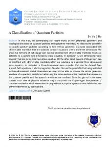
1. Introduction hand small enough to allow for quantum mechanical interference effects to be observable. More precisely, we can define the mesoscopic regime by the requirement of a preserved phase coherence of the propagating wave. In this situation, many interesting phenomena show up on length scales that are smaller than the phase coherence length Lφ . Three different theoretical approaches are regularly applied to the description of these phenomena: diagrammatic techniques [2], random matrices [10] and supersymmetry [24]. Although these descriptions may differ in their assumptions and ranges of validity, they all have one thing in common: the idea of ensemble averaging. Since it is in general impossible to model the influence of one specific configuration of defects, one tries to obtain average results for many such configurations. The diagrammatic technique is a microscopic approach, i.e. it is based on the description of scattering events off single impurities. These scattering events are connected to scattering paths to describe multiple scattering. Different scattering paths are then sorted in Feynman diagrams, and the ensemble average is carried out by integrating over the scattering centers’ positions. In contrast, random matrix theory takes a macroscopic approach: instead of calculating specific scattering paths, one considers the ensemble of possible scattering matrices of the system and derives probability distributions of the matrix elements from general symmetry considerations. Finally, the supersymmetric approach uses a Lagrangian formalism to derive the desired quantities. All three approaches have their strengths and weaknesses, depending mainly on the geometry of the underlying problem. As we will focus on the propagation of quantum particles in a waveguide geometry in this thesis, we choose to make use of the random matrix approach, which will turn out to be well suited for studying quasi one-dimensional systems. Having discussed the theory side, let us now turn to the physics involved. When a disordered medium is illuminated by a laser beam, the light gets scattered randomly, resulting in a predominantly diffusion-like propagation inside the medium. The measured intensity I on output of the medium then shows a sharply peaked, granular structure - the so-called speckle pattern, as shown in figure 1.1. In most cases, the associated intensity distribution (in other words, the distribution over the statistical ensemble) is very well described by the Rayleigh law [53]: � � 1 I P (I) = exp − , I I
(1.1)
where I denotes the mean value of the output intensity. Equation (1.1) is based on the assumption of an entirely random superposition of waves on the output of the medium, featuring a classical diffusion process. It cannot account for correlations between different output directions that survive the ensemble average, and, consequently, in certain situations a more elaborate description is needed. Hereafter
4
from this functional shape has to be determined. Our setup was custom designed for this purpose and consists of 256 photosensitive diodes attached to an arc with a diameter of 1.2 m in order to get sufficient angular resolution over a range of j"j < 65% [21]. Here, the resolution is !1% for j"j > 10% and 0.14% for j"j < 10% . In addition, the central 1.1. The mesoscopic scale part of the backscattering cone, j"j < 3% , was measured
FIG. 1. Measurements of coherent backscattering for two dif-
Figure 1.1.: Left: Speckle patternferent produced a laser beam illuminating a rough samples.by Open symbols: R700 with an average particle " surface, from [97]. diameter Right: ofCoherent backscattering for T iOTiClosed symbols: 250 nm which yields k‘ & 2:5.cones 2 6:3. All with an average diameter of 540 nm and This k‘" & figure powder (open circles)Pure and pure T i powder (filled circles). were done with circularly polarized light at a is taken from [81]. measurements wavelength 2#=k & 590 nm. The insets show electron micrographs of R700 and Ti-pure.
of a picosecond ligh is measured. From pulses, the path len obtained directly [9 modified with a mo works at a wavelen !20 ps. In order to tions, the TOF histo pulse shape of the pulses, albeit strong may lead to disturb this purpose we mea a sample for each ex indiscriminate back convoluted with the give the path leng peaked pulse as it shows the path leng terized in Fig. 1 com be seen in Fig. 2(a absorption [17] fits contrast, the path le shows marked devi ticular, we observe with photons stayin pected from a purely scaling theory [17]. an increased total normalized to total
063904-2 we give three examples of important manifestations of phase coherent transport in disordered media, which cannot be described by the simple model (1.1).
Coherent backscattering Consider a disordered medium illuminated by a collimated beam. When measuring the reflected intensity in the backscattering direction, constructive interference between counter-propagating multiple scattering paths inside the medium leads to an enhancement of the reflected intensity over the value expected for a purely diffusive process by a factor of two. Around the exact backscattering direction, the angle-resolved intensity profile exhibits a narrow cone. This phenomenon is known as the coherent backscattering effect.2 An example of a backscattering cone for light is shown in figure 1.1. This effect was first predicted theoretically in the late 1960’s by [90, 9], and observed experimentally in the 1980’s [3, 37, 33, 98].
Universal conductance fluctuations In small (mesoscopic) metallic devices, preserved phase coherence of electronic wave functions leads to a sensitive dependence of the conductance G on the specific 2
Note that in the case of electronic transport in metals, the constructive interference between counter-propagating paths is also responsible for a reduction of the conductivity, a phenomenon usually referred to as weak localization [40].
5
40 Atomic density (atoms µm–1)
30 20
PHYSICAL10 REVIEW LETTERS –0.8 1,000
–0.4
0.0
d
0.4
rms width (mm)
NUMsEa. 26 VoLUME 56, 1. Introduction
100
1.0 0.5
0.0 0
0.8
VR = 0 VR ≠ 0 1 t (s)
10
0 10
l
l
l
2
4
6
1 –0.8
0
aB (tesl
0.0 3. 0.4 0.8 FIG. Normalized correlation z (mm) ments of magnetic field and gate vo of Fig. 2. a, A small BEC field at of exponential ing datalocalization. FIG. 2. Dimensionless conductance vs Figure magnetic 1 | Observation 4 the conductance G with varying magFigure 1.2.: Left: Reproducible variation of indicat3 10 atoms) is formed in a hybrid trap that is the combination of a segment three gate voltages, for the inversion layer (1.7 netic field conductance for different horizontal gate voltages in a metal-oxide-silicon field ef- confinement, and optical ensuring a strong transverse orvariations ofvGwaveguide, ed in Fig. 1, showing aperiodic that foll discussion and equations a loose magnetic longitudinal trap. A localized weak disordered optical potential, fect transistor, taken from [78]. Right: Exponentially density der e~/h. transversely invariant over thein atomic cloud, is superimposed if one or(disorder more d our Ina random case, profile of a Bose Einstein condensate expanding potential, with the chemical potential m of amplitude VR low in comparison in tem being studied exceedthe initia taken from [15].
B (tesla)
–0.4
L;„
BEC). b, When the longitudinal trap is switched off, the BEC starts W'can L or widthimaging be divid deviation a root-mean-square expanding conductance SG, and then localizes,length as observed by direct of the a and false fluorescence of the atoms irradiated by a resonant probe. In function4 W/L;„phase-coherent b,subu correlation C that and a conductance colour images and sketched profiles are for illustration purposes; they are positions of thefield impurities. This creates fluctuations one disorder typically SGt e2/h, and gate- from differing displacement byrealization magnetic depends on c , d , Density profiles (red) of the localized BEC one not exactly to scale. to another, known as universal fluctuations [32]. They are calledseries-parallel uniadd classical ofsemi-log 4 VG. sumsin linear function The conductance voltage displacement c) and (d) coordinates. In the inset in second afterCrelease, (use versal, since the variance of the conductance G (defined as the inverse resistivity) relative sizet fluctuation bined(rms) we display the root-mean-square width of the of profile versus time to respect products of deviations, computed here d with of a mesoscopic conductor reads with (VR ? 0) and without (VR 5 0) disordered potential.2N This shows that 2e2/h. lute size SG the average value for each magnetic field trace. This the stationary regime is reached after 0.5 s. The diamond at t 5 1 s the ar characterizing from average isolates random interference phenomenacorresponds panel of d. Blue lines in cph to the data shownchange in c and the main 2 thenlines cor interference Figexponential fits the wings,random and correspond to the(1.2) straight blue in dependences of the conductance on gate δG2voltage. = G 0 , to 15 d . The narrow central profiles (pink) represent the trapped condensate several flux quanta h/e in the ure 3 shows the correlation function (normalized to before release (t 5 0 s).
(G),
58
M=
=
=M'
8,
coherent subunit. (Reference 4 that includes the data tn Fig. 2, the variance) for a set 2 3 with G = 2e /h only depending on the fundamental constants con- 4h/e for a 892 0 teristice and fluxh. isA =2. with (G) =11.7e /h, and SG =0.65e2/h. The correla©2008 Macmillan Publishe venient way to observe conductance fluctuations consists in varying an external wide. ) The chemical potential c has half-widths tion function 8, = 0.48 T and magnetic field. This way, one can directly influence the phase shift between sucing the energy correlation of t V. These correspond respectively to a VG, =0.22 cessive scattering events, and thus effectively sample many disorder realizations. sponds to the lesser of E, =~2k the seen the area can of be fluxresult of 3.of5h/e segment, magnetic The such in a technique in figure 1.2 (left). The variation the latter case applying in al inversionfield B with the magnetic and to a ofchemical-potential the conductance as achange function in of the is erratic, but entirely Experimentally, L and W'are =1.6 meV=4. 5kaT. layer of p,reproducible. tron micrographs of the devices, In order to compare such experimental results with from Eq. (1) and the average con coherence to consider the phasereferred theory, it 3isIn necessary condensed matter physics G0 is usually to as the quantum of conductance. It corof L, IV, and terms Inthethe absence ofof within the device. magnetic impurity responds to conductance a perfect electronic conductor withset. only aIn single transmission theoretical describ predictions channel. scattering, the length scale for destruction of phase inrelevant case L;„<) reduce t formation is set by the inelastic diffusion length L = (D7 )'lz, where D = vFl/d is the diffusion conSg= [max(L;„,W)/L]'l'[L; d with respect to the mean stant for 6 dimensionality is the inelastic scattering time. For free path l, and p, = min(n 2t/~;„, several ka two-dimensional electron-electron scattering, ~;„ is 8, = (2.4h/e)/[L;„min( O', proportional to D/T and D is proportional to the average conductance of a square (g~) = (G) L/W(e /h). For the data set corresponding Weak-localization experiments on large MOSFETs'8 L. Thus p, m, so that W'& L;„& and parallel arrays of long, narrow MOSFET chanof slightly more than one quant
,
7;„
,
L
1.2. Non-classical light in disordered media Anderson localization The phenomenon of localization of electronic wave functions in certain disordered media, today known as Anderson localization, was discovered by Anderson in 1958, [5]. This is in sharp contrast with the usual (classical transport) picture [23] according to which transport is always described by a diffusion process, as mentioned above, and, as such, the conductance G of a dirty, metallic sample follows Ohmic behavior, G ∝ Ld−2 (for a d-dimensional cube with side length L). According to Anderson’s theory, the eigenfunctions of a particle on a three-dimensional disordered lattice undergo a phase transition when increasing the disorder strength: Above a certain energy, the so-called mobility edge, they decay exponentially in space, leading to an exponential decay of the conductance, G ∼ e−L/ξ , on a characteristic length scale ξ known as the localization length. Abrahams, Anderson, Licciardello and Ramakrishnan [1] put this result and other preliminary works in a larger picture, as they developed the scaling theory of localization in 1979. In their seminal paper, they used a very appealing scaling theory to explain this phase transition in three dimensions. In one or two dimensions, on the other hand, any wave function is localized in the infinite medium [1]. However, in a finite medium eigenfunctions may appear delocalized, if the length of the system is smaller than the localization length, i.e. if L/ξ � 1. In the opposite limit L/ξ � 1 transport is suppressed (G → 0). In this respect, ξ can be interpreted as the average distance over which a particle can propagate when Anderson localization occurs. It was later discovered that the concept of Anderson localization is not restricted to electronic wave functions, but also applies to classical wave scattering described by a Helmholtz equation [31]. The disorder is then imprinted in the dielectric constant [87, 38]. Anderson localization was demonstrated for ultrasound in 1990 [91], for microwaves in 1991 [30], later for light in 1997 [92, 72], 2006 and 2007 [81, 74], and for matter waves in 2008 [15, 68]. In the latter case, a Bose Einstein condensate is released into a disordered optical lattice, which suppresses the expansion of the condensate for a certain time. The exponentially localized density profile of the condensate, and, in other words, its atomic wave function, is then analyzed by means of optical absorption (see right part of figure 1.2).
1.2. Non-classical light in disordered media As pointed out above, mesoscopic effects are wave interference effects. For the case of light this means that they can be formulated theoretically on the level of wave
7
frequency for transport and scattering sample "D=L2 ' e optical frequency "! ' pproximation to employ a "!# for the optical field. we calculate the spectral fluctuations j"I"!#j2 $ ^ d "I"!# $ %!( ! a^ y "!#& ) joint operator. The spectral d in the experiment, and for btain [4]
in 2 ! "!#j
v "!#j2 # * j"I!
v "I! "!#j2 ;
(4)
uum contribution
0 b0 "!#"a ^ b! "!##y i; !
(5)
respectively. Assuming the electric field amplitudes can be described by a circular Gaussian process (short range correlations) [13], it follows that the fourth-order correlation function can be expressed in terms of the second-order correlation function, which implies hhCSN ab ""!#ii! $ f"##;
between the input field in tions from each of the vac0 7]. We note that ha^ b! "!# ) e [in the following referred an also be described with cuum contributions. In the v "!#j2 $ we have j"I!
!#j2SN
!#j
2
!#j2TN
!#j2
$ T!ab ; $ T!ab2 ;
(8a)
2 hhCTN (8b) ab ""!#ii! $ f "## ! 4f"##; 1. Introduction p!!!! p!!!! where f"## $ #=%cosh" ## * cos" ##& is the secondorder correlation function given in [14] with # $ 2L2 "!=D. The experimental setup is outlined in Fig. 1. A frequency tunable titanium-sapphire laser was used to probe the random multiple scattering samples. The lasers’ amplitude noise spectrum was found to be limited by shot noise above '1:5 MHz and dominated by technical noise
Titania random powder Ti:sapphire laser
recorded a frequency speckle pattern. In total, 200 noise spectra were measured at equally spaced optical frequencies with a frequency step of about 0:5 THz: From the complete measurement series the autocorrelation function was obtained. Figure 2 displays two measurements of the total transmission of noise through samples with different thicknesses. Two frequency regimes are apparent in the data: below %1 MHz and above %1:5 MHz, corresponding to
was obtained. In the speckl pare the behavio in Fig. 4 displa noise by varying We compute t Eq. (2) for both decay with freq correlation func due to stray in single speckle s well described b [16]. The corre
Integrating sphere D2
Spectrum analyzer
SA D1
FIG. 1 (color online).
Experimental setup for measuring the
FIG. 2 (color online).
Total transmission of noise as a function
Figure Left:noise Experimental to measure thefrequency noise level of light transmission1.3.: of quantum through a multiplesetup scattering of measurement ! for two differentpropagatsample thickmedium. Two different measurements were carried out by innesses. The spectral densities were recorded with a resolution ing through a disordered medium. A sample of length L consisting of FIG. 3 (color onl serting either detector D1 or D2. The total transmission was bandwidth of 30 kHz and a video bandwidth of 10 kHz and by (6b) recorded with an integrating sphere onto detector D1. With T iO2 powder is illuminated from theeachleft, the transmitted quantum noise as averaging traceand 100 times. Radically different intentransmisdetector D2, the noise in a single speckle spot was measured. linear fit to the sions are observed for technical noise (below 1 MHz) compared sity is integrated and measured. Right: Total transmission of noise transmission of c to shot noise (above 1:5 MHz). The spikes around 1:3 MHz are 153905-2 different scales in to oscillationsΩ. in the Two detectordistinct power supplynoise and arelevabanas function of the measuredduefrequency doned in the analysis. els can be distinguished, corresponding to dominating shot noise (for and quantum noi 153905-3 Ω > 0.5 MHz) and to technical noise (Ω < 0.5 MHz), respectively. Both graphs are taken from [43]. (6a)
mechanics, where light is described by the Maxwell equations and its quantized nature is neglected. Starting with several theoretical papers around the turn of the millennium [60, 61], the influence of disorder on the nonclassical, particle-like character of quantum light has become the subject of numerous theoretical and experimental studies. As an example, we show in figure 1.3 a study on the noise level of (coherent) laser light transmitted through a disordered medium consisting of T iO2 powder carried out in 2005. The right-hand side thereof shows the total transmission of classical and quantum noise through the disordered medium as a function of the measured frequency Ω. One can clearly see two distinct regions. For a measured frequency Ω < 0.5 MHz, the noise level is dominated by the technical noise of the laser, whereas for Ω > 0.5 MHz it is dominated by the shot noise, which reflects the granularity of quantum light, and is caused by a variation of the number of photons that hit the detector in a measurement time interval. Figure 1.3 shows that a disordered medium transmits quantum noise much better than classical noise. This reveals that both sources of noise can be distinguished by their distinct scaling behaviors with the length of the disordered medium. While the interplay between the quantum properties of light and disorder is far from being entirely understood, it has soon been recognized that some quantum properties of the incident light do survive the ensemble average, and can be traced
8
1.3. Motivation of the thesis back by analyzing the photocount statistics or correlation functions of the transmitted or backscattered field. Previous studies have so far turned to two different aspects of the quantum character of light: The first group focused on the effects of disorder on photon number fluctuations [43, 44, 8, 42, 77], i.e. for different types of propagating light, for instance squeezed light or photonic Fock states. They assumed the light to be incident in one mode, but allowed for varying photon numbers or squeezing parameters. We will discuss another example thereof in more detail in chapter 4. The other group [88, 14, 58, 62, 19] studies the impact of disorder on the propagation of entanglement.
1.3. Motivation of the thesis In the present thesis, we investigate the propagation of a simple, however strongly quantum, object - a pair of non-interacting particles - in a disordered waveguide. This poses an interesting problem, because it constitutes the easiest system to examine different aspects of many-body physics, and allows more specifically to understand the role of quantum statistics of propagating particles (bosonic or fermionic) for the transport in disordered environments. The issue of many-body effects in quantum transport and Anderson localization has raised considerable interest in the recent literature [39, 71, 46] where it was discussed in the context of photonic lattices or beamsplitter arrays, i.e. in strictly one-dimensional settings. The waveguide geometry extends this discussion to a quasi one-dimensional system which allows for the formation of a diffusive regime of transport. On the other hand, the non-separability of the incident wave function, i.e. the initial entanglement, is also affected by multiple scattering, and we may ask how it is degraded by the interaction with the medium. Conversely, we may also examine whether multiple scattering can actually create entanglement between the particles. The theory we develop in this thesis lies within a rich and promising experimental field in optics, where it is already possible to create pairs of photons in desired initial states [63] and to detect them after transition through a disordered medium [62]. Beyond optics, disordered waveguides for ultracold atoms can be produced with laser light. For bosons, the interaction between atoms can be effectively tuned using Feshbach resonances [7, 70], and for fermions by use of spin-polarized particles [21]. It should thus be possible to create effectively non-interacting particles, such that the particle statistics should become observable for both types of particles as described by our theory.
9
1. Introduction
1.4. Structure of the thesis The thesis is structured as follows: after the present short introduction, we will discuss the theoretical background necessary to describe our system in chapter 2. This includes an introduction to the terminology of transport in disordered waveguides, and to random matrix theory in quantum transport, and a recollection of the quantization of bosonic and fermionic fields. Then we will examine the behavior of an important observable, the single-mode current, in chapter 3. This observable is mainly interesting in view of the interplay between quantum and disorder noise, as described above. Guided by these results, we will focus on a more sophisticated object, the coincidence rate, in chapter 4. There, we will discuss correlations rather than fluctuations to see the influence of the particle statistics. Chapter 5 provides a discussion on the relation between entanglement and disorder, and the subtle issues connected to it. Finally, we will summarize our findings in chapter 6.
10
2. Background The system we will focus on in this thesis consists of a quasi one-dimensional disordered waveguide. Quantum particles - bosons as well as fermions - can be injected on either side, propagate through the sample, and be detected on the other side. Defects or impurities, the origin of the disorder in the system, scatter the quantum particles. As we will discuss in this chapter, the precise origin of the disorder is not essential in this problem, as transport properties only depend on a small set of macroscopic parameters, and not on the microscopic details of the disorder. Depending on the scattering strength, propagation of the particles can be either diffusive or, possibly, completely suppressed. In the present chapter, we will first introduce the basic concepts of the physics of disorder. Then, in section 2.2, we will turn to the mathematical description of the physical system and introduce the central concepts of this work, most prominently the notion of the scattering matrix. Next, having presented the general framework to describe transport in disordered media, in section 2.3 we will focus our attention on the concept of random matrices in scattering systems. This theory will enable us to perform ensemble averages on many such systems and calculate probability distributions of quantum mechanical observables. The quantum mechanical background of field quantization will be shortly outlined in the subsequent section 2.4. Since the system introduces two types of statistics, the quantum mechanical and the ensemble statistics, we will finally discuss the relation between the two of them in different measurement setups in section 2.5.
2.1. Transport in a disordered waveguide This short section introduces the main concepts that were developed in the past years to describe disordered systems. Due to the enormous research effort in this area originating from many fields of modern physics, any exhaustive description lies way beyond the scope of this thesis. Hence, we will here restrict ourselves to a concise presentation of a few important ideas. In today’s picture of electronic transport, it is due to delocalized electrons close to the Fermi energy, while the majority of electrons is localized around the nuclear cores. The elastic scattering off impurities and defects, i.e. scattering without energy exchange between electron and impurity, plays the dominant role in the
11
2. Background
Figure 2.1.: Sketch of a quasi one-dimensional scattering setup with disorder. Impurities are indicated by grey balls. The relevant length scales in this geometry are the radius r, the total length L, and the elastic mean free path �. transport properties of the delocalized electrons (at zero temperature) [34, 83]. On mesoscopic length scales, i.e. for sample lengths L smaller than the electronic coherence length Lφ , an electron in the conduction band can be described by a quantum mechanical wave function. As we pointed out in the introduction, this preserved phase coherence manifests itself in new phenomena stemming from interference effects, thus defining the mesoscopic regime. When electron interactions can be neglected, such a system is described by the time-independent singleparticle Schr¨odinger equation, which has a mathematical structure similar to the classical Helmholtz equation [87, 38]. Accordingly, such interference effects are not restricted to quantum systems, but also show up in classical wave mechanics, provided that wave coherence is preserved.
2.1.1. Length scales Apart from Lφ , four important length scales come into play in the problem of elastic impurity scattering in a disordered medium (see figure 2.1): the transverse diameter 2r of the medium, its total length L, the mean free path �, i.e. the average distance between two successive scattering processes,1 and the localization length ξ, i.e. the typical length beyond which the effects of Anderson localization starts affecting transport. Depending on their ratios, these parameters determine the macroscopic behavior of the system. In this work, we will focus on the case of a quasi one-dimensional geometry, i.e. 1
In general, another length scale needs to be taken into account, the transport mean free path �∗ , defined as the average distance over which the memory of an incident direction of the wave is lost. In the following, we will only consider the case where � = �∗ , which is fulfilled for scatterers of size much smaller than the wavelength (i.e. isotropic scattering, see [2]).
12
2.1. Transport in a disordered waveguide the transverse extension is much smaller than the total length, r � L.
2.1.2. The Thouless conductance In 1977, Thouless [84], in view of describing the universal transport properties of disordered systems of finite size, put forward the concept of the so-called dimensionless conductance or Thouless number g, introduced as the ratio δE , (2.1) ∆E where ∆E denotes the mean spacing of the energy levels in the medium. When the boundaries of the system are changed, the energy levels may shift by a finite value δE. Thouless argued that Anderson localization sets in when this shift becomes smaller than the mean level spacing, i.e. for g < 1, since the conductor can then be decomposed into only weakly correlated blocks containing localized wave functions (see figure 2.2). In this case, transport is suppressed. On the other hand, when g � 1, eigenfunctions are extended, and thus allow for the formation of propagating wave packets. These extended wave functions facilitate transport of particles or energy. The great significance of the Thouless number stems from the fact that it is directly proportional to the Ohmic conductance, which is a common, measurable quantity.2 Within this picture, the Thouless number can also be determined from the well known Landauer formula (see [20]) g=
g = tr{tt† },
(2.2)
where t denotes the transmission matrix, which will be discussed in more detail in section 2.2.
2.1.3. Different types of transport As pointed out in section 2.1.1, depending on the relative length scales in our system, we can distinguish three distinct regimes of transport: Ballistic transport When the mean free path is larger than the system length, � > L, electrons hardly ever scatter off impurities and one speaks of ballistic transport. In this regime the transmission matrix in (2.2) simply equals the unit matrix. The dimensionless conductance g is thus given by the dimension of the matrix, i.e. the number of modes N in the waveguide [20], g = N. 2
(2.3)
Note that the concept of the dimensionless conductance is not restricted to electronic systems, but also applies, more generally, to any wave propagation problem in extended media.
13
2. Background
Figure 2.2.: Illustration of the Thouless criterion: the localized wave function in the left graph is hardly affected at all by a change of the boundary conditions. Hence, δE � ∆E ⇒ g � 1. The extended wave function in the right graph on the other hand is strongly affected by such a change, and can effectively mediate transport across the sample. Diffusive transport When the mean free path is much smaller than the system length, � � L, any particle traveling through the medium undergoes many scattering events (“multiple scattering”), and its propagation can be effectively described by a diffusion process. This picture holds as long as L � ξ, with ξ the localization length. In this regime, the dimensionless conductance is given by g=
N� � 1. L
(2.4)
In the following, 1/g will naturally appear as the small parameter of the perturbation theory describing deviations from diffusive behavior, known as weak localization corrections. In the context of electronic conductors, the latter usually manifest themselves as a reduction of the conductivity [20], and are sometimes interpreted as signs of the onset of Anderson localization (see e.g. [3]), thus defining a weakly localized transport regime. We will also use this terminology in the following. In other words, we denote the regime of finite g as weakly localized, while the terminology diffusive regime will be restricted to the limit g → ∞, in which interference can be safely neglected. Localized regime When g becomes smaller than unity, Anderson localization sets in according to the Thouless criterion. The remaining conductance in a finite medium is then giving by the remaining overlap of the localized wave functions
14
2.2. Mode discretization in the waveguide geometry Single scattering
Ballistic regime
g
Weakly localized regime
Localized regime
�
ξ
N
1
Incoherent transport
Lφ
L
Figure 2.3.: The different transport regimes and their evolution with respect to the system length L and the dimensionless conductance g. with the boundaries of the medium, resulting in an exponential decay of the conductance: � � L g ∼ exp − . (2.5) ξ In the geometry of a waveguide, considered in this thesis, the dimensionless conductance g evolves continuously from the limiting cases (2.3) and (2.4) to (2.5) as the system length L varies. This is schematically depicted in figure 2.3. An exact calculation of g, for any L, usually requires numerical simulations. In this thesis we will give analytical results for the three limiting cases, and only resort to numerics in the crossover regimes.
2.2. Mode discretization in the waveguide geometry So far, we have only been concerned with transport in a very general setting. In this section, we now turn to the kind of system we are aiming at - a disordered waveguide. We introduce the concept of mode discretization, which will enable us to formulate the rest of the theory needed. The following reasoning is applicable to the propagation of classical waves (light, microwaves), where one needs to solve the scalar Helmholtz equation,3 as well as to quantum mechanical waves like atomic matter waves or electronic waves, where the Schr¨odinger equation is to be solved. For the sake of clarity, however, we will adopt the terminology of electronic transport in a disordered conductor in this 3
In considering the scalar Helmholtz equation, we neglect the polarization of the waves, which is justified in the point scattering limit [2].
15
2. Background
Figure 2.4.: A disordered conductor connected to two perfect leads with circular cross section. The longitudinal direction is parametrized by the variable x, the transverse distance to the symmetry axis by ρ, and angles to the figure plane by φ. section. Consider a disordered conductor with transverse diameter 2r and length L � r (Fig. 2.4). The electron is required to maintain its phase coherence throughout the propagation, i.e. we require L � Lφ , where Lφ is the electron’s coherence length. As discussed in chapter 1, this requirement defines the so-called mesoscopic regime of propagation. The electronic wave function satisfies the single-particle Schr¨odinger equation −�2 ∆ψ(�r) + V (�r)ψ(�r) = Eψ(�r), 2m
(2.6)
where V (�r) is the disordered potential describing the scattering region of the waveguide. In writing equation (2.6), we have neglected spin degrees of freedom. This is justified as long as we do not consider spin-dependent scattering, e.g. scattering off magnetic impurities. This additional degree of freedom is however to be considered in the total number of modes later on. We further assume perfectly reflecting boundary conditions at the outer surface of the waveguide: ψ(ρ = r, φ, x) = 0,
∀φ, x.
(2.7)
Outside the disordered region, the conductor is a perfect lead, and V (�r) = 0. Equation (2.6) then reduces to the Laplace equation, which can be solved analytically. Making use of the problem’s rotationally invariant geometry around the
16
2.3. Random matrices in scattering systems x-axis, we make the ansatz4 ψ ± (ρ, φ, x) = f (ρ)e±ikx ·x .
(2.8)
In the longitudinal direction, we simply have plane waves, whose propagation direction is indicated by the ± sign, with “+” refering to the propagation from left to right and “−” vice versa. The solutions for f (ρ) turn out to be Bessel functions of the first kind, and the boundary condition (2.7) enforces a discretization of the transverse wave number, kρ . These discrete wave numbers define the modes of the waveguide. More specifically, for any given incoming wave vector �k, related to the transverse and the longitudinal components kρ and kx through k 2 = kρ2 + kx2 =
2mE , �2
(2.9)
there is a finite number of modes n = 1 . . . N , for which both kρ and kx are real. (n) (n) It is this set of pairs {kρ , kx }n=1...N that determines the transport properties. When a particle is injected on a given side of the conductor, its wave function is given by a superposition of these modes, and the way it gets transmitted or reflected depends on the way these modes are coupled due to the scattering from impurities. Finally, since particles can be injected either from the left or from the right, transport is described by a total number of 2N modes (N for left to right and N for right to left).
2.3. Random matrices in scattering systems Random matrices are used in countless applications, ranging from the problem of energy level statistics of large nuclei [93, 94, 95, 96] to economic sciences [66]. Common to all random matrix theories is the idea that the ensemble of matrices is “as random as possible” [49]. In other words, one first determines the ensemble of matrices from which one draws the samples by considering the underlying symmetries of the problem. Within these ensembles, the probability distribution is chosen “as random as possible”, although the origin of randomness heavily depends on the system in question. In the following, we will only be concerned with the specific case of scattering systems. The purpose of this section is to give a brief introduction to random 4
We thus restrict our discussion for the sake of simplicity to the case of vanishing angular momentum. In general, there are modes with non-vanishing angular momentum present, and they contribute to the total number of modes. However, their consideration only technically complicates the following discussion, but does not alter the qualitative result.
17
2. Background
Figure 2.5.: The incoming (black) and outgoing fluxes (red). The scattering matrix S maps incoming on outgoing fluxes, (I, I � ) → (O, O� ), while the transfer M matrix maps (I, O) → (I � , O� ). matrix theory for transport in such systems, and sketch the main steps of the derivations of the necessary formulae, while emphasizing physical intuition rather than mathematical rigor. Details can be found in the given literature.
2.3.1. The polar decomposition In quasi one-dimensional scattering systems, two equivalent descriptions are regularly used, the scattering matrix and the transfer matrix formalism. Due to the 2N modes introduced in 2.2, the scattering matrix is a 2N × 2N matrix, � � r t� S= , (2.10) t r� where we have decomposed S into N × N transmission and reflection matrices, t (from left to right), t� (from right to left) and r (from right to right), r� (from left to left), respectively. The scattering matrix connects incoming and outgoing fluxes: � � � � I O S = , (2.11) I� O� whereas the transfer matrix, M=
�
m1 m2 m3 m4
�
,
(2.12)
connects fluxes on the left of the medium to fluxes on the right (see figure 2.5): � � � � � I I M = . (2.13) O O� Both descriptions of a scattering system in terms of S or M are equivalent, and
18
2.3. Random matrices in scattering systems their building blocks matrices are connected through the relations [82], m1 = (t† )−1 , m2 = r� (t� )−1 , m3 = −(t� )−1 r, m4 = (t� )−1 .
(2.14)
We will make use of both formalisms in this chapter. Since measurements are carried out on outgoing fluxes only, the scattering matrix formalism is the natural choice to describe the propagation of quantum particles through a waveguide. However, it has an important shortcoming: there is no easy combination law for scattering matrices connected to each other at their ends, unlike for transfer matrices. Indeed, assume you divide a waveguide into two pieces a and b, each with transfer matrices Ma and Mb . Then, the transfer matrix of the whole system is simply given by M = Ma · Mb . Of course, due to the complexity of the system, there is, in general, little hope of obtaining an exact solution for the combined effect of many scatterers in a particular configuration. This problem can however be circumvented by looking at the statistical properties of an ensemble of disordered systems rather than looking at specific realizations. This can be done by describing the system in terms of an ensemble of random scattering matrices, the statistics of this ensemble being imposed by certain symmetry properties for the disorder, as we will now show. Flux conservation Since we assume the scattering to be elastic (see the introduction to section 2.1), there is no exchange of energy between particle and scattering center, and consequently also no absorption. Thus, any particle entering the waveguide will leave it eventually. Therefore, the amplitudes of incoming and outgoing fluxes must be the same, |I|2 + |I � |2 = |O|2 + |O� |2
⇒ S · S† = ,
(2.15)
i.e. the scattering matrix is unitary.5 In the transfer matrix formalism, the terms in (2.15) are rearranged as |I|2 − |O|2 = |O� |2 − |I � |2 ,
(2.16)
which means that M is a pseudo-unitary matrix [49], i.e., it conserves the so-called hyperbolic norm of the vector (I, O) of fluxes on each side. Alternatively, the flux conservation condition can be formulated by introducing the 2N × 2N matrix � � 1 0 Σz = . (2.17) 0 −1 In this case, flux conservation reads [49]
M † Σz M = Σz . 5
(2.18)
Note that the argument does not work the other way around: unitarity of the scattering matrix does NOT imply elastic scattering.
19
2. Background Time reversal invariance From here on, we will additionally assume the dynamics to be invariant under time reversal. Physically, time reversal symmetry can be broken either by a magnetic field or magnetic impurities,6 and we will not consider such situations in the present work. Technically, time reversal amounts to the exchange of incoming and outgoing fluxes, together with complex conjugation of the amplitudes. By introducing a new matrix � � 0 1 Σx = , (2.19) 1 0 time reversal invariance can be expressed as [49] M ∗ = Σx M Σx ,
(2.20)
where M ∗ denotes the complex conjugate of the transfer matrix M . The polar decomposition We now introduce an important decomposition of the transfer matrix (2.12), the polar decomposition. Given the constraints (2.18) and (2.20), we decompose √ M into √ independent unitary N × N matrices U and V , and diagonal matrices τ −1 and τ −1 − 1, such that: 7 √ � �� √ �� � −1 −1 − 1 U 0 τ τ V 0 √ √ M= . (2.22) 0 U∗ 0 V∗ τ −1 − 1 τ −1 The eigenvalues {τn }n=1...N of the diagonal matrix τ are called eigenparameters or transmission eigenvalues of M . This decomposition reflects the number of free parameters N · (2N + 1) (N 2 parameters from each U and V , N from the {τn }). One can physically interpret the U - (V -) matrix as the matrix connecting the lead modes on the right (left) side of the waveguide to the modes inside. Each of these internal modes is characterized by the transmission eigenvalue τ , which gives the probability for transmission, and the corresponding probability for reflection, 1−τ . The different eigenvalues τn can be associated with the “conducting channels” of the waveguide, as the conductance, given by the Landauer formula (2.2), reads � G = G0 tr{tt† } = G0 τn , (2.23) n
6 7
i.e. impurities that carry a magnetic moment. A similar decomposition exists for the scattering matrix (2.10), � �� √ �� T √ U 0 − 1−τ √ τ U √ S= 0 V 0 τ 1−τ
20
0 VT
�
.
(2.21)
2.3. Random matrices in scattering systems where G0 = e2 /h is the quantum of conductance [20]. In this picture, the conductance G is given by the sum of the transmission coefficients over all incoming and outgoing modes, which simply reduces to the sum over the transmission eigenvalues. Consequently, it follows that it is mostly the distribution of these eigenvalues which bears information about the transport properties of the medium. This has to be contrasted with the U - and V -matrices, which, on the other hand, merely account for the geometry of the medium, and for the coupling of the scattering volume to the leads.
2.3.2. The invariant measure Having introduced the polar decomposition (2.22), our next task consists in finding the probability distributions of the unitary matrices U and V , as well as those of the eigenparameters τ . As a first guess, we could assign equal a-priori-probability to each pseudo-unitary matrix M fulfilling the constraints (2.18) and (2.20), i.e. we could look for a probability measure dPL (M ) with dPL (M1 ) = dPL (M2 ) for any two elements M1 , M2 of the pseudo-unitary group G, defined by (2.16). Mathematically, this amounts to choosing the Haar measure dµ(M ) of G for dPL (M ). It is defined by the invariance property dµ(M ) ≡ dµ(M · M0 ) and dµ(M ) ≡ dµ(M0 · M ),
(2.24)
for any element M0 of the pseudo-unitary group G. In 1988, Mello, Pereira and Kumar [49] derived an explicit expression in the parametrization (2.22), dµ(M ) = J({x}) with J({x}) =
� a 1, it is entangled. Now consider the reduced density matrix acting on Hilbert space H1 . From (5.4), we immediately obtain (1)
�ˆ
≡ tr2 {|ψ��ψ|} =
M � i=1
λi |i�1 �i|1 .
(5.5)
� Because of probability conservation, tr{ˆ �} = 1, we know that M i=1 λi = 1. This allows us to use the purity of the reduced density matrix, often called participation ratio [85], to detect entanglement, S(ψ) ≡ tr{(ˆ �(1) )2 } = 1
⇔
|ψ� is a product state.
(5.6)
Entanglement of indistinguishable particles Now we can come back to the case of indistinguishable particles. As S(ψ) appears in (5.3), one may be tempted to use this quantity as an entanglement quantifier. But consider the state |ψ4 � = ˆb†q0 ˆb†q1 |0�,
(5.7)
with one boson in mode q0 and one in q1 . Clearly, this state is not entangled, it is simply the symmetrized product of the wave functions of modes q0 and q1 ,1 1
For example, in the space representation state (5.7) reads ��r1�r2 |ψ4 � = φq0 (�r1 )φq1 (�r2 ) + φq0 (�r2 )φq1 (�r1 ),
(5.8)
˜ r1 ) · φ(� ˜ r2 ). which cannot be brought into the form φ(�
75
5. Entanglement and disorder and correlations arising from this symmetrization cannot be attributed to entanglement. Nevertheless, the reduced density matrix of (5.7) reads �ˆ(1) =
� 1 �ˆ† bq0 |0��0|ˆbq0 + ˆb†q1 |0��0|ˆbq1 , 2
(5.9)
which results in the participation ratio S(ψ4 ) = 1/2 < 1. This means that the symmetrization of the wave function destroys the applicability of the participation ratio as an entanglement quantifier. But still, we can at least detect some entangled states.� Assuming we are free to change the mode basis by unitary transformations2 ˆ bˆ� q = l Uql bl , we can find a basis for any two-particle state |ψ�, such that it appears in the so-called standard form [85] M
1 � ˆ† 2 |ψ� = √ cq (bq ) |0�. 2 q=1
(5.10)
We already encountered the number M as the participation number in (3.40). In the context of entanglement theory, it is usually called the rank of the state |ψ�. It is known [85] that for a rank larger than two, the state is entangled, while a rank-two state may or may not be entangled. Hence, if we were able to give a lower bound on S(ψ) for a rank-two state, we would be able to detect at least some entangled states. To this end, we consider a state of rank two with standard form 1 |ψ� = √ (c1 (ˆb†q1 )2 + c2 (ˆb†q2 )2 )|0�. 2
(5.11)
The participation ratio for this parametrization reads S(ψ) = |c1 |4 + |c2 |4 ,
(5.12)
so we can assume without loss of generality that c1 and c2 are both real. We further require that the norm of the state is unity, which translates into c21 + c22 = 1. Thus, we have to minimize L(c1 , c2 ) = c41 + c42 + λ(c21 + c2 − 1),
(5.13)
where we introduced the Lagrange multiplier λ. Minimization of the Lagrange function, i.e. setting δc1 L = δc2 L = δλ L = 0, leads to 1 |c1 | = |c2 | = √ . 2 2
(5.14)
This by itself is a delicate point, since the modes may be spatially separated, rendering the transformation U non-local. This issue will be discussed in section 5.2.
76
5.1. Variance of the bosonic coincidence rate
δ
d
Figure 5.1.: Spatial separation of different modes in the far field � outside the waveguide. Two speckle spots are separated by δ ∼ d2 /N [14]. This means, the lowest value S(ψ) can take for a state of rank 2 is 1/2. Therefore, any state with S(ψ) < 1/2 must be of rank > 2, which in turn means it is entangled. In conclusion, the notion of entanglement in a system of indistinguishable particles is a very intricate problem, as the non-separability of the wave function conflicts with the need to (anti-)symmetrize it. Still, by measuring the variance of the coincidence rate (5.3) and of the single mode current (3.50), it is possible to draw conclusions about initial entanglement, since it allows to access the purity as well as the participation ratio of the initial state. At the same time, by calculating the weak localization corrections of both quantities, we demonstrate the need to carefully take them into account. Indeed, depending on the value of g, these corrections may be become of the same order of magnitude as the very effect we are looking for: in the limit of very large g, we can access the purity P = tr{ˆ �2 } of the incident state through [14]
P =
var(�Iˆ2 �) var(�Iˆ1 �) − 2 . 4 (�/N L)4 (2�/N L)2
(5.15)
Including interference effects, this expression reads �
4 P = tr{ˆ � } 1+ 3g 2
�
8 + tr{ˆ �(1) }2 + O g
�
1 g2
�
> tr{ˆ �2 },
(5.16)
i.e. one would consequently overestimate the purity for finite g.
77
5. Entanglement and disorder
5.2. Mode entanglement So far, we discussed entanglement between particles, and we have seen that it is quite cumbersome to work with. Now, we would like to argue that it may be more insightful to consider the modes rather than the quantum particles as the basic quantities. Indeed, as we pointed out at the beginning of this chapter, we are envisioning an optical waveguide as a realization of this model, since it can be realized experimentally. But this also implies that measurements are carried out in the far field of the system (see figure 5.1). If the distance d between waveguide and detector is much larger than the radius of the waveguide, the size of a speckle spot created by the outgoing mode k is roughly d2 /N [14]. Hence, a transformation mixing the different modes such as the one we used to derive the standard form (5.10) also mixes spatially separate points. It has to be considered non-local, therefore changes the degree of entanglement. Consequently, the theory of particle entanglement, even though it is perfectly applicable, may not give us much insight about quantum correlations in the system. It is the geometry of the system that fixes the modes, and thus these modes have to be regarded as the fundamental quantities in our problem, not the particles [85]. They are spatially distinct, and we can immediately apply the whole theory for distinguishable particles. Mathematically speaking, we recall that our system consists of 2N Fock spaces (see section 2.4.1), H = H1 ⊗ · · · ⊗ H2N ,
(5.17)
and the issue of entanglement in such a system can thus be regarded as the problem of entanglement in a 2N -body problem [4]. Let us only give an example: if we want to know whether mode 1 is entangled with the other modes, we have to trace over all the modes except the first one: �ˆ1 = tr2,...,N {ˆ �} ≡
∞ �
n2 ,...,n2N =0
�n2 , . . . , n2N |ˆ �|n2 , . . . , n2N �
(5.18)
Consider an outgoing state of the form (2.63), which results from the transmission of a general two-particle state (2.58) across the waveguide. Tracing over all the outgoing modes except mode 1 yields � (1) � � � ∗ ∗ ∗ �ˆ1 = 1 − 2 �qq� S1q S1q �q1 q2 q1� q2� S1q1 S1q � S1q2 S1q � |0��0| � + 1 2 q,q �
q1 ,q2 ,q1� ,q2�
� � � (1) � † ∗ ∗ ∗ ˆ ˆ + 2 �qq� S1q S1q �q1 q2 q1� q2� S1q1 S1q � S1q2 S1q � b1 |0��0|b1 � − 1 2 q,q �
+
78
1 2
�
q1 ,q2 ,q1� ,q2�
� † �2 � � ∗ ∗ ˆ |0��0| ˆb1 2 . �q1 q2 q1� q2� S1q1 S1q � S1q2 S1q � b1 1 2
q1 ,q2 ,q1� ,q2�
(5.19)
5.3. Summary The particle number is no longer conserved in this approach. Since the scattering matrix elements are on the order of |Skq |2 = �/(N L) � 1 (see section ??), the vacuum contribution comprises the dominant part of state (5.19). Apart from this vacuum contribution, we obtain a single-particle contribution and a two-particle part. To get a first idea of how this quantity can be interpreted, we calculate its purity in the diffusive regime, i.e. we treat the scattering matrix elements as Gaussian variabes (3.15). The result reads �� � �2 � �4 � �4 �6 � � � � � tr{(ˆ �1 ) 2 } ≈ 1 − 4 + 12 +8 tr{(ˆ �(1) )2 } + O . NL NL NL NL (5.20) It turns out that the average purity of the reduced state (5.19) is close to one, but diminished by small corrections in �/(N L). In this picture, the multiple scattering does create a certain, however small, amount of entanglement between the outgoing modes. This average degree of entanglement depends only weakly on the incident state, which only contributes in second order via tr{(ˆ �(1) )2 } [the purity of the full incident state also contributes at higher orders of �/(N L)]. It would interesting to investigate how this result is affected by interference effects. As we have seen in (5.3), these weak localization corrections are rather detrimental for the detection of entanglement, since they complicate the measurement of the precise values of tr{ˆ �2 } or tr{(ˆ �(1) )2 }. On the other hand, one could argue that the correlations between the transport channels that cause the weak localization corrections should create entanglement between the modes outside the waveguide. Besides, in the regime of Anderson localization, fluctuations tend to become very large. one might speculate that there could be a substantial percentage of disorder realizations that is actually very efficient at inducing entanglement, even though the average amount of entanglement as in (5.20) may be very small. Another interesting possibility consists in the generalization of the quantities presented here, e.g. in the investigation of entanglement between modes on different sides of the waveguide or the like.
5.3. Summary We discussed the possibility of observing signatures of input state quantum correlations. We argued that this is possible in general, although such measurements might be difficult in strongly disordered system, when weak localization corrections effects tend to hide entanglement signatures. Furthermore, we argued that due to the geometry of the system, it may be more insightful to examine entanglement between the modes. The question to wether or
79
5. Entanglement and disorder not it is possible to detect and utilize this type of entanglement remains however open.
80
6. Conclusion and Outlook In this thesis we studied the propagation of pairs of quantum particles through a disordered waveguide. Due to the particles’ scattering from impurities inside the medium, the state of the particles after the propagation is drastically affected. Thus, the larger part of the present work was devoted to the study of how initial properties of the particles show up in transmission measurements. To that end we first examined the single-mode current, and later the coincidence rate. At the end of the work, we also discussed the possibility of creating quantum correlations between the particles by multiple scattering, and gave some preliminary results. In our study of the single-mode current, we focused on the disorder regime of weak localization. We derived explicit expressions for the probability distributions of both the single-mode current and the integrated current. By comparison with the formulae for the variances obtained from perturbative expansions of exact quantities, it was shown that both distributions reproduce the exact results very well for incident states with small participation numbers. On the other hand, for very large participation numbers the disorder causes a universal noise level that cannot be reproduced by the approximate expressions of the probability distributions. With regards to our initial motivation, it was shown that the single-mode current, as a single-particle observable, cannot distinguish between bosonic or fermionic particles traveling through the waveguide, nor can it detect initial quantum coherences. The measurement outcome is the same for highly entangled states and their incoherent counterparts. As the single-mode current turned out to be not very insightful in the study of initial properties of the particles, we turned to the examination of coincidence measurements. These measurements show a dramatic dependence on the bosonic or fermionic character of incident particles. In the localized regime, the bosonic quantum correlation function was shown to grow exponentially with the length of the waveguide, whereas the fermionic one breaks down exponentially. Both effects can be understood as manifestations of the Pauli exclusion principle and boson bunching, respectively. As can be seen from the random matrix theory of disordered waveguides (see section 2.3.3), the transmission channels group into open channels with transmission probability close to unity, and closed channels with very small transmission probabilities. When the disorder gets stronger, ever fewer
81
6. Conclusion and Outlook channels belong to the first group, such that eventually only one relatively open channel is left. Hence, if one fermion already occupies this channel, the other one has to resort to another channel with very small transmission probability, and the correlation function measured at the output collapses. For bosons, on the other hand, the presence of another particle increases the probability of the first one to use the same channel because of bosonic bunching. Consequently, the bosonic correlation function is enhanced by a factor of two compared to the correlation function for distinguishable particles. These findings constitute the main results of the thesis. In further work, it would be interesting to extend the study of bosonic and fermionic behavior in the localized regime to higher dimensions. So far, the study of Anderson localization focused on single-particle wave functions and neglected the (anti-)symmetrization of many-particle wave functions. The influence of the particle symmetry on the localization properties might also affect the (Anderson) phase transition in three dimensions, since we have already observed that distinguishable particles react less strongly to interference effects in our quasi one-dimensional model. The biggest obstacle to overcome in this respect is the generalization of random matrix theory of quantum transport to higher dimensions. To date, only phenomenological approaches are available [55, 56]. Another possible extension of this work consists in the propagation of entangled photons through turbid atmospheres [69]. While the present random matrix theory is based microscopically on a white noise model, an application of this problem would require an extension to the specific noise model present in turbid atmospheres. In chapter 5 we addressed the problem of non-classical correlations in the initial bosonic wave function. It was first discussed that the variance of the coincidence rate may reveal initial entanglement. This statement was however moderated, as a closer examination showed that the indistinguishability of the particles and the symmetrization of the wave function that comes along with it complicates the notion as well as the detection of entanglement in this system. Finally, we demonstrated that, in principle, multiple scattering can create entanglement between the different modes of the waveguide. A more elaborate treatment of this issue could, on the one hand, try to assess whether there is an appreciable fraction of disordered systems that is efficient at creating mode entanglement, and which transport regime is most successful at doing so. On the other hand, it would be essential to come up with strategies to extract and use this mode entanglement.
82
A. Averages on the unitary group In this appendix, we derive the formalism necessary to evaluate expressions of the kind � a1 α1 ,...,al αl Qb1 β1 ,...,bm βm = dµ(U )(ub1 β1 . . . ubm βm )(u∗a1 α1 . . . u∗al αl ), (A.1) � � � � and dµ(U ) exp ca1 a2 ua1 b u∗a2 b , (A.2) a1 ,a2
where the integration measure µ(U ) is the invariant measure of the unitary group. We here summarize the solutions for both problems, which can be found in the literature. While there are exact solutions for expression (A.1) available up to m = 4 [48], we can at least report of approximate solutions for the marginal distribution of single matrix elements [64] to solve equation (A.2).
A.1. The marginal distribution The following line of arguments can be found in greater detail in [64]. By definition, the Haar measure µ(U ) is invariant under group transformations U → U 0 · U or U · U 0 ,
(A.3)
for any U 0 from the unitary group. Assume that the joint probability distribution of the first line of U is known, dp(U11 , . . . , U1N ) = p(U11 , . . . , U1N ) dU11 . . . dU1N .
(A.4)
Because of the invariance property (A.3), it needs to stay unaffected by multiplication of any unitary matrix U 0 from the right, which mixes the elements of this line. Since the only invariant for any U 0 is the norm of the vector composed of these elements, we can conclude p(U11 , . . . , U1N ) ∝ δ(1 −
N � a=1
|U1a |2 ).
(A.5)
83
A. Averages on the unitary group Integrating out all the elements except U11 yields � �N −2 � � �� p(U11 ) ∝ 1 − |U11 |2 = exp (N − 2) ln 1 − |U11 |2 .
(A.6)
Obviously, this distribution peaks at |U11 | = 0, so we obtain a good estimate by expanding the logarithm to first order. In the limit of very large N , this gives the final result of a Gaussian distribution with zero mean and variance 1/N , � � � N p(U11 ) → exp −N |U11 |2 , N → ∞. (A.7) 2π Higher order corrections can be estimated to be on the order of O(1/N ) [64].
A.2. Exact averages The evaluation of an expression of the kind (A.1) can be reduced to solving a set of linear equations by making use of the unitarity of the matrices. The unitarity leads to three conditions we can impose on the Q-terms. Condition I: ,...,al αl Because of the invariance property of the Haar measure (A.3), Qab11βα11,...,b needs m βm to be invariant under multiplication from left and right by any unitary matrix U 0 . This means: a� α ,...,a� α
,...,al αl 0∗ 1 1 l l Qab11βα11,...,b = (u0b1 b�1 . . . u0bm b�m )(u0∗ a1 a�1 . . . ual a�l )Qb� β1 ,...,b�m βm m βm 1
a α� ,...,a α�
0 0 0∗ 0∗ = Qb11β �1,...,bml βlm � (uβ � β1 . . . uβ � βm )(uα� α1 . . . uα� αl ) m 1 1 l 1
(A.8) (A.9)
(Summation over indices appearing twice is understood). If we choose u0ab = δab eiθab , (A.8) and (A.9) turn into ,...,al αl ,...,al αl Qab11βα11,...,b = exp[i(θa1 α1 + · · · + θal αl ) − i(θb1 β1 + · · · + θbm βm )]Qab11βα11,...,b m βm m βm (A.10) ,...,al αl = exp[i(θb1 β1 + · · · + θbm βm ) − i(θa1 α1 + · · · + θal αl )]Qab11βα11,...,b , m βm (A.11)
which must be satisfied for all choices of phases, since equations (A.8) and (A.9) must be true for any unitary matrix. Therefore, the phases must cancel, and we find that the sets of Greek and Roman indices must coincide, {α} ≡ {β} and {a} ≡ {b}. This yields m = l.
84
A.2. Exact averages Condition II: Matrix elements commute with each other. Therefore, Q needs to be invariant under permutations of both upper and lower index pairs, since this only amounts to rearranging the order of unitary matrix elements in the integral: a
α
,...,a αl��
,...,al αl l αl 1�� l�� Qab11βα11,...,b = Qab11�αβ11,...,a = Qb11β��1 ,...,b � ,...,bm� βm� m βm m βm
,
(A.12)
where the permutations are indicated by primes. Condition III: � ∗ The matrix U is unitary, i.e. b uab ubc = δac . A contraction of the Q-terms therefore produces Kronecker-δ’s as well: � a α ,...,a α ,...,am αm Qa11 β11,...,bmmβmm = δα1 β1 Qab22βα22,...,b (A.13) m βm a1
The number of equations one needs to solve in order to evaluate (A.1) increases very fast with the order of the polynomial, i.e. the number of matrix elements under consideration. Mello obtained results up to m = 4 [48], from which we only list the ones relevant for our calculations in this work, and compare with the results when treating the matrix entries as Gaussian variables. m=1 The result reads Qaα bβ =
1 δab δαβ , N
(A.14)
and exactly agrees with the Gaussian approximation obtained from the distribution (A.7). Since the Gaussian distribution neglects any correlations between distinct matrix element, it can only give a non-vanishing result when the two matrix elements ubβ and u∗aα coincide, which gives the Kronecker δ’s δab δαβ . m=2 For m = 2, we find Qab11βα11,b,a22βα22 = −
N2 1
1 (δa b δα β δa b δα β + δa1 b2 δα1 β2 δa2 b1 δα2 β1 ) −1 1 1 1 1 2 2 2 2
N (N 2 − 1)
(δa1 b1 δa2 b2 δα1 β2 δα2 β1 + δa1 b2 δa2 b1 δα1 β1 δα2 β2 ).
(A.15)
85
A. Averages on the unitary group The first line in equation (A.15) coincides with the result of the Gaussian approximation (A.7), since this part of the result gives contributions to the case when pairs of matrix elements coincide, just like above in (A.14). However, the second line gives a correction that is smaller by a factor 1/N . It stems from correlations between distinct matrix elements that are neglected by the Gaussian approximation. However, since in our case N is very large, this encourages us to believe that treating the matrix element as independent Gaussian variables in the previous section A.1 is a very good approximation. m=4 The number of terms we obtain for the exact solution grows as (m!)2 . This means that for m = 4 already, we have to deal with 576 terms. However, as in the case m = 2, terms of different orders of magnitude are involved. In the limit N � 1, which is of most interest in our study, it is sufficient to keep track of only the largest 24 terms, which are obtained by permuting the variables and the complex conjugates simultaneously. This result is given by N 4 − 8N 2 + 6 · (A.16) N 2 (N 2 − 1)(N 2 − 4)(N 2 − 9) (δa1 b1 δα1 β1 δa2 b2 δα2 β2 δa3 b3 δα3 β3 δa4 b4 δα4 β4 + δa1 b1 δα1 β1 δa2 b2 δα2 β2 δa4 b3 δα4 β3 δa3 b4 δα3 β4 + δ a 1 b 1 δ α 1 β1 δ a 3 b 2 δ α 3 β2 δ a 2 b 3 δ α 2 β3 δ a 4 b 4 δ α 4 β4 + δ a 1 b 1 δ α 1 β1 δ a 3 b 2 δ α 3 β2 δ a 4 b 3 δ α 4 β3 δ a 2 b 4 δ α 2 β4 + δ a 1 b 1 δ α 1 β1 δ a 4 b 2 δ α 4 β2 δ a 2 b 3 δ α 2 β3 δ a 3 b 4 δ α 3 β4 + δ a 1 b 1 δ α 1 β1 δ a 4 b 2 δ α 4 β2 δ a 3 b 3 δ α 3 β3 δ a 2 b 4 δ α 2 β4 + δ a 2 b 1 δ α 2 β1 δ a 1 b 2 δ α 1 β2 δ a 3 b 3 δ α 3 β3 δ a 4 b 4 δ α 4 β4 + δ a 2 b 1 δ α 2 β1 δ a 1 b 2 δ α 1 β2 δ a 4 b 3 δ α 4 β3 δ a 3 b 4 δ α 3 β4 + δ a 2 b 1 δ α 2 β1 δ a 3 b 2 δ α 3 β2 δ a 1 b 3 δ α 1 β3 δ a 4 b 4 δ α 4 β4 + δ a 2 b 1 δ α 2 β1 δ a 4 b 2 δ α 4 β2 δ a 3 b 3 δ α 3 β3 δ a 1 b 4 δ α 1 β4 + δ a 3 b 1 δ α 3 β1 δ a 1 b 2 δ α 1 β2 δ a 2 b 3 δ α 2 β3 δ a 4 b 4 δ α 4 β4 + δ a 3 b 1 δ α 3 β1 δ a 1 b 2 δ α 1 β2 δ a 4 b 3 δ α 4 β3 δ a 2 b 4 δ α 2 β4 + δ a 3 b 1 δ α 3 β1 δ a 2 b 2 δ α 2 β2 δ a 1 b 3 δ α 1 β3 δ a 4 b 4 δ α 4 β4 + δ a 3 b 1 δ α 3 β1 δ a 2 b 2 δ α 2 β2 δ a 4 b 3 δ α 4 β3 δ a 1 b 4 δ α 1 β4 + δ a 3 b 1 δ α 3 β1 δ a 4 b 2 δ α 4 β2 δ a 1 b 3 δ α 1 β3 δ a 2 b 4 δ α 2 β4 + δ a 3 b 1 δ α 3 β1 δ a 4 b 2 δ α 4 β2 δ a 2 b 3 δ α 2 β3 δ a 1 b 4 δ α 1 β4 + δ a 4 b 1 δ α 4 β1 δ a 1 b 2 δ α 1 β2 δ a 2 b 3 δ α 2 β3 δ a 3 b 4 δ α 3 β4 + δ a 4 b 1 δ α 4 β1 δ a 1 b 2 δ α 1 β2 δ a 3 b 3 δ α 3 β3 δ a 2 b 4 δ α 2 β4 + δ a 4 b 1 δ α 4 β1 δ a 2 b 2 δ α 2 β2 δ a 1 b 3 δ α 1 β3 δ a 3 b 4 δ α 3 β4 + δ a 4 b 1 δ α 4 β1 δ a 2 b 2 δ α 2 β2 δ a 3 b 3 δ α 3 β3 δ a 1 b 4 δ α 1 β4 + δa4 b1 δα4 β1 δa3 b2 δα3 β2 δa1 b3 δα1 β3 δa2 b4 δα2 β4 + δa4 b1 δα4 β1 δa3 b2 δα3 β2 δa2 b3 δα2 β3 δa1 b4 δα1 β4 ).
Qab11βα11,b,a22βα22,b,a33βα3 ,b3 ,a4 β44α4 =
Other contributions stemming from correlation between distinct matrix elements are suppressed by a factor of at least 1/N 2 .
86
B. Moments of the total transmission These calculations can be found in much greater detail in [52]. T2
��
N a=1 τa
�2
The goal of this appendix is to evaluate observables of the kind = �N 2 or T2 = a=1 τa in the weakly localized transport regime (see section 2.1.3). For convenience, the following calculations will be carried out in the basis of the new variables λ, defined by τ = 1/(1 + λ). The starting point of our calculations is the DMPK equation (2.31): � � N ∂ 2 � ∂ ∂ ps ({λ}) ps ({λ}) = λa (1 + λa )J({λ}) , ∂s N + 1 a=1 ∂λa ∂λa J({λ})
(B.1)
where s = L/� is the length of the waveguide L in units of the mean free path � and J({λ}) is the Jacobian originating from the transition from the space of transfer matrices into the space of transmission eigenvalues (see section 2.3.2). Multiplying both sides of (B.1) by a function F ({λ}) of the eigenvalues and integrating over the coordinates λ1 , . . . , λN yields � ∂F ∂F �� N +1 ∂ ∂F 1 � λa (1 + λa ) ∂λa − λb (1 + λb ) ∂λb F = λa (1 + λa ) + , (B.2) 2 ∂s ∂λ 2 λ − λ a a b a a�=b which is an evolution equation for the function F ({λ}) having � the form of a integrop differential equation. For the special case of F = T = [ a 1/(1 + λ)]p , this equation turns into (N + 1)
∂ p T = −pT p+1 − pT p−1 T2 + 2p(p + 1)T p−2 (T2 − T3 ), ∂s
(B.3)
� with Tk = a 1/(1 + λa )k . A close look at equation (B.3) reveals that it is not a closed system of equations, so there is no way to solve this problem exactly. But in the limit N � 1, one can expand these functions in power series of N and then
87
B. Moments of the total transmission solve for each power of N separately.1 T p = N p fp0 (s) + N p−1 fp1 (s) + . . . T p T2 = N p+1 gp+1,0 (s) + N p gp+1,1 (s) + . . .
(B.4) (B.5)
After a lengthy, but straighforward calculation, this approach yields Np ps3 p − N p−1 + [(11p − 9)s8 + . . . ]N p−2 + . . . , p p+2 (1 + s) (1 + s) 90(1 + s)p+6 (B.6) 7 2s3 + 6s2 + 6s + 3 p (10p + 4)s + . . . T p T2 = N p+1 − N + . . . .. (B.7) (1 + s)p+4 45(1 + s)p+7 Tp =
In the diffusive limit s � 1, it is sufficient to only keep the leading order terms in s for each power of N . This results in an expansion in powers of g = N �/L. We here state the functions necessary for our work: � �4 � �3 � �2 N� 4 N� 14 N � 4 T ≈ − + , (B.8) L 3 L 9 L � �2 � � N � 2 N� 13 N � T2 ≈ − + , (B.9) L 3 L 45 L N� 1 1 L T ≈ − + , (B.10) L 3 45 N � � �3 � �2 2 N� 34 N � T 2 T2 ≈ − , (B.11) 3 L 45 L 2 N� 4 T2 ≈ − (B.12) 3 L 45 � �2 4 N� 2 (T2 ) ≈ , (B.13) 9 L � �2 8 N� T T3 ≈ , (B.14) 15 L 272 N � T4 ≈ . (B.15) 135 L
1
This procedure is legitimate in the weakly localized regime, where N � L/�, but not in the localized regime, where N � L/� (see section 2.1.3).
88
Bibliography [1] Abrahams, E., Anderson, P. W., Licciardello, D. C., and Ramakrishnan, T. V. Scaling theory of localization: Absence of quantum diffusion in two dimensions. Phys. Rev. Lett. 42, 673 (1979). [2] Akkermans, E. and Montambaux, G. Mesoscopic physics of electrons and photons. Cambridge University Press (2007). [3] Albada, M. P. V. and Lagendijk, A. Observation of weak localization of light in a random medium. Phys. Rev. Lett. 55, 2692 (1985). [4] Amico, L., Fazio, R., Osterloh, A., and Vedral, V. Entanglement in manybody systems. Rev. Mod. Phys. 80, 517 (2008). [5] Anderson, P. W. Absence of diffusion in certain random lattices. Phys. Rev. 109, 1492 (1958). [6] Andrews, M., Mitra, P., and deCarvalho, R. Tripling the capacity of wireless communications using electromagnetic polarization. Nature 409, 316 (2001). [7] Aspect, A. and Inguscio, M. Anderson localization of ultracold atoms. Physics Today 62, 30 (2009). [8] Balog, S., Zakharov, P., Scheffold, F., and Skipetrov, S. E. Photocount statistics in mesoscopic optics. Phys. Rev. Lett. 97, 103901 (2006). [9] Barabanenkov, Y. N. Wave corrections to the transfer equation for “back” scattering. Radiophysics and Quantum Electronics 16, 65 (1973). [10] Beenakker, C. W. J. Random-matrix theory of quantum transport. Rev. Mod. Phys. 69, 731 (1997). [11] Beenakker, C. W. J. and Rajaei, B. Exact solution for the distribution of transmission eigenvalues in a disordered wire and comparison with randommatrix theory. Phys. Rev. B 49, 7499 (1994). [12] Beenakker, C. W. J. and Rejaei, B. Nonlogarithmic repulsion of transmission eigenvalues in a disordered wire. Phys. Rev. Lett. 71, 3689 (1993).
89
Bibliography [13] Beenakker, C. W. J. and Sch¨onenberger, C. Quantum shot noise. Physics Today 56, 37 (2003). [14] Beenakker, C. W. J., Venderbos, J. W. F., and van Exter, M. P. Two-photon speckle as a probe of multi-dimensional entanglement. Phys. Rev. Lett. 102, 193601 (2009). [15] Billy, J., Josse, V., Zuo, Z., Bernard, A., Hambrecht, B., Lugan, P., Clement, D., Sanchez-Palencia, L., Bouyer, P., and Aspect, A. Direct observation of anderson localization of matter waves in a controlled disorder. Nature 453, 891 (2008). [16] Blanter, Y. and Buttiker, M. Shot noise in mesoscopic conductors. Physics Reports 336, 1 (2000). [17] Bronshtein, I. Handbook of mathematics. Springer (2007). [18] Caselle, M. Distribution of transmission eigenvalues in disordered wires. Phys. Rev. Lett. 74, 2776 (1995). [19] Cherroret, N. and Buchleitner, A. Entanglement and Thouless times from coincidence measurements across disordered media. Phys. Rev. A 83, 033827 (2011). [20] Datta, S. Electronic transport in mesoscopic systems. Cambridge studies in semiconductor physics and microelectronic engineering. Cambridge University Press (1997). [21] DeMarco, B., Bohn, J. L., Burke, J. P., Holland, M., and Jin, D. S. Measurement of p-wave threshold law using evaporatively cooled fermionic atoms. Phys. Rev. Lett. 82, 4208 (1999). [22] Dorokhov, O. N. Solvable model of multichannel localization. Phys. Rev. B 37, 10526 (1988). [23] Drude, P. Zur Elektronentheorie der Metalle. Annalen der Physik 306, 566 (1900). [24] Efetov, K. Supersymmetry in disorder and chaos. Cambridge University Press (1999). [25] Engel, G. S., Calhoun, T. R., Read, E. L., Ahn, T.-K., Mancal, T., Cheng, Y.-C., Blankenship, R. E., and Fleming, G. R. Evidence for wavelike energy transfer through quantum coherence in photosynthetic systems. Nature 446, 782 (2007).
90
Bibliography [26] Fink, M. Imaging: Sharper focus by random scattering. Nature Photonics 4, 269 (2010). [27] Froufe-Perez, L. S., Garcia-Martin, A., Cwilich, G., and Saenz, J. J. Fluctuations and correlations in wave transport through complex media. Physica A: Statistical Mechanics and its Applications 386, 625 (2007). [28] Froufe-Perez, L. S., Garcia-Mochales, P., Serena, P. A., Mello, P. A., and Saenz, J. J. Conductance distributions in quasi-one-dimensional disordered wires. Phys. Rev. Lett. 89, 246403 (2002). [29] Froufe-Perez, L. S., Garcia-Mochales, P., Serena, P. A., Mello, P. A., and Saenz, J. J. A Monte Carlo approach to determine conductance distributions in quasi-one-dimensional disordered wires. Microelectronics Journal 36, 893 (2005). [30] Genack, A. Z. and Garcia, N. Observation of photon localization in a threedimensional disordered system. Phys. Rev. Lett. 66, 2064 (1991). [31] John, S. Electromagnetic absorption in a disordered medium near a photon mobility edge. Phys. Rev. Lett. 53, 2169 (1984). [32] Kaplan, S. B. and Hartstein, A. Universal conductance fluctuations in narrow si accumulation layers. Phys. Rev. Lett. 56, 2403 (1986). [33] Kaveh, M., Rosenbluh, M., Edrei, I., and Freund, I. Weak localization and light scattering from disordered solids. Phys. Rev. Lett. 57, 2049 (1986). [34] Kittel, C. Introduction to solid state physics. Wiley (2005). [35] Kogan, E. and Kaveh, M. Random-matrix-theory approach to the intensity distributions of waves propagating in a random medium. Phys. Rev. B 52, R3813 (1995). [36] Krauth, W. Statistical Mechanics: Algorithms and Computations. Oxford Master Series in Statistical, Computational, and Theoretical Physics. Oxford University Press (2006). [37] Kuga, Y. and Ishimaru, A. Retroreflectance from a dense distribution of spherical particles. J. Opt. Soc. Am. A 1, 831 (1984). [38] Lagendijk, A. and van Tiggelen, B. A. Resonant multiple scattering of light. Physics Reports 270, 143 (1996).
91
Bibliography [39] Lahini, Y., Bromberg, Y., Christodoulides, D. N., and Silberberg, Y. Quantum correlations in two-particle Anderson localization. Phys. Rev. Lett. 105, 163905 (2010). [40] Lee, P. A. and Ramakrishnan, T. V. Disordered electronic systems. Rev. Mod. Phys. 57, 287 (1985). [41] Levi, L., Rechtsman, M., Freedman, B., Schwartz, T., Manela, O., and Segev, M. Disorder-enhanced transport in photonic quasicrystals. Science 332, 1541 (2011). [42] Lodahl, P. Quantum noise frequency correlations of multiply scattered light. Optics Letters 31, 110 (2006). [43] Lodahl, P. and Lagendijk, A. Transport of quantum noise through random media. Phys. Rev. Lett. 94, 153905 (2005). [44] Lodahl, P., Mosk, A. P., and Lagendijk, A. Spatial quantum correlations in multiple scattered light. Phys. Rev. Lett. 95, 173901 (2005). [45] Mandel, L. and Wolf, E. Optical coherence and quantum optics. Cambridge University Press (1995). [46] Mayer, K., Tichy, M. C., Mintert, F., Konrad, T., and Buchleitner, A. Counting statistics of many-particle quantum walks. Phys. Rev. A 83, 062307 (2011). [47] Mehta, M. Random matrices. vier/Academic Press (2004).
Pure and applied mathematics. Else-
[48] Mello, P. A. Averages on the unitary group and applications to the problem of disordered conductors. J. Phys. A: Math. Gen. 23, 4061 (1990). [49] Mello, P. A., Pereyra, P., and Kumar, N. Macroscopic approach to multichannel disordered conductors. Annals of Physics 181, 290 (1988). [50] Mello, P. A. and Pichard, J.-L. Maximum-entropy approaches to quantum electronic transport. Phys. Rev. B 40, 5276 (1989). [51] Mello, P. A. and Shapiro, B. Existence of a limiting distribution for disordered electronic conductors. Phys. Rev. B 37, 5860 (1988). [52] Mello, P. A. and Stone, A. D. Maximum-entropy model for quantummechanical interference effects in metallic conductors. Phys. Rev. B 44, 3559 (1991).
92
Bibliography [53] Mirlin, A. D., Pnini, R., and Shapiro, B. Intensity distribution for waves in disordered media: Deviations from Rayleigh statistics. Phys. Rev. E 57, R6285 (1998). [54] Moustakas, A. L., Baranger, H. U., Balents, L., Sengupta, A. M., and Simon, S. H. Communication through a diffusive medium: Coherence and capacity. Science 287, 287 (2000). [55] Muttalib, K. A. and Klauder, J. R. Generalized Fokker-Planck equation for multichannel disordered quantum conductors. Phys. Rev. Lett. 82, 4272 (1999). [56] Muttalib, K. A., Markoˇs, P., and W¨olfle, P. Conductance distribution in strongly disordered mesoscopic systems in three dimensions. Phys. Rev. B 72, 125317 (2005). [57] Nielsen, M. and Chuang, I. Quantum computation and quantum information. Cambridge Series on Information and the Natural Sciences. Cambridge University Press (2000). [58] Ott, J. R., Mortensen, N. A., and Lodahl, P. Quantum interference and entanglement induced by multiple scattering of light. Phys. Rev. Lett. 105, 090501 (2010). [59] Paˇskauskas, R. and You, L. Quantum correlations in two-boson wave functions. Phys. Rev. A 64, 042310 (2001). [60] Patra, M. and Beenakker, C. W. J. Excess noise for coherent radiation propagating through amplifying random media. Phys. Rev. A 60, 4059 (1999). [61] Patra, M. and Beenakker, C. W. J. Propagation of squeezed radiation through amplifying or absorbing random media. Phys. Rev. A 61, 063805 (2000). [62] Peeters, W. H., Moerman, J. J. D., and van Exter, M. P. Observation of two-photon speckle patterns. Phys. Rev. Lett. 104, 173601 (2010). [63] Peeters, W. H., Renema, J. J., and van Exter, M. P. Engineering of twophoton spatial quantum correlations behind a double slit. Phys. Rev. A 79, 043817 (2009). [64] Pereyra, P. and Mello, P. A. Marginal distribution of the S-matrix elements for Dyson’s measure and some applications. J. Phys. A: Math. Gen. 16, 237 (1983).
93
Bibliography [65] Pichard, J.-L. and Sarma, G. Finite size scaling approach to Anderson localisation. Journal of Physics C: Solid State Physics 14, L127 (1981). [66] Potters, M., Bouchaud, J.-P., and Laloux, L. Financial applications of random matrix theory: Old laces and new pieces. Science & Finance (CFM) working paper archive 500058, Science & Finance, Capital Fund Management (2005). [67] Risken, H. The Fokker-Planck equation: methods of solution and applications. Springer series in synergetics. Springer (1996). [68] Roati, G., D’Errico, C., Fallani, L., Fattori, M., Fort, C., Zaccanti, M., Modugno, G., Modugno, M., and Inguscio, M. Anderson localization of a noninteracting Bose-Einstein condensate. Nature 453, 895 (2008). [69] Roux, F. S. Infinitesimal-propagation equation for decoherence of an orbital-angular-momentum-entangled biphoton state in atmospheric turbulence. Phys. Rev. A 83, 053822 (2011). [70] Sanchez-Palencia, L. and Lewenstein, M. Disordered quantum gases under control. Nat Phys 6, 87 (2010). [71] Sansoni, L., Sciarrino, F., Vallone, G., Mataloni, P., Crespi, A., Ramponi, R., and Osellame, R. Two-particle bosonic-fermionic quantum walk via 3D integrated photonics. ArXiv e-prints (2011). 1106.5713. [72] Scheffold, F., Lenke, R., Tweer, R., and Maret, G. Localization or classical diffusion of light? Nature 398, 206 (1999). [73] Scholak, T., Mintert, F., Wellens, T., and Buchleitner, A. Chapter 1 - transport and entanglement. In Eicke R. Weber, M. T. and W¨ urfel, U. (editors), Quantum Efficiency in Complex Systems, Part I: Biomolecular systems, volume 83 of Semiconductors and Semimetals, pages 1 – 38. Elsevier (2010). [74] Schwartz, T., Bartal, G., Fishman, S., and Segev, M. Transport and Anderson localization in disordered two-dimensional photonic lattices. Nature 446, 52 (2007). [75] Sheng, P. Introduction to wave scattering, localization and mesoscopic phenomena. Springer Publishing Co., 2nd edition (2006). [76] Simon, S. H., Moustakas, A. L., Stoytchev, M., and Safar, H. Communication in a disordered world. Physics Today 54, 38 (2001). [77] Skipetrov, S. E. Quantum theory of dynamic multiple light scattering in fluctuating disordered media. Phys. Rev. A 75, 053808 (2007).
94
Bibliography [78] Skocpol, W. J., Mankiewich, P. M., Howard, R. E., Jackel, L. D., Tennant, D. M., and Stone, A. D. Universal conductance fluctuations in silicon inversion-layer nanostructures. Phys. Rev. Lett. 56, 2865 (1986). [79] Smolka, S., Huck, A., Andersen, U. L., Lagendijk, A., and Lodahl, P. Observation of spatial quantum correlations induced by multiple scattering of nonclassical light. Phys. Rev. Lett. 102, 193901 (2009). [80] Stensby, J. Ee420/500/603 random signals and noise class note archives. URL http://www.ece.uah.edu/courses/ee420-500/. [81] Stoerzer, M., Gross, P., Aegerter, C. M., and Maret, G. Observation of the critical regime near Anderson localization of light. Phys. Rev. Lett. 96, 063904 (2006). [82] Stone, A. D., Mello, P. A., Muttalib, K. A., and Pichard, J.-L. Random matrix theory and maximum entropy models for disordered conductors. In Altshuler, B. L., Lee, P. A., and Webb, R. A. (editors), Mesoscopic Phenomena in Solids, volume 30 of Modern Problems in condensed matter sciences, chapter 9, pages 369 – 448. Elsevier Science Publishers B.V. (1991). [83] Thouless, D. J. Electrons in disordered systems and the theory of localization. Physics Reports 13, 93 (1974). [84] Thouless, D. J. Maximum metallic resistance in thin wires. Phys. Rev. Lett. 39, 1167 (1977). [85] Tichy, M. C., Mintert, F., and Buchleitner, A. Essential entanglement for atomic and molecular physics. Journal of Physics B: Atomic, Molecular and Optical Physics 44, 192001 (2011). [86] van Grondelle, R. and Novoderezhkin, V. I. Photosynthesis: Quantum design for a light trap. Nature 463, 614 (2010). [87] van Tiggelen, B. A. and Kogan, E. Analogies between light and electrons: Density of states and Friedel’s identity. Phys. Rev. A 49, 708 (1994). [88] van Velsen, J. L. and Beenakker, C. W. J. Transition from pure-state to mixed-state entanglement by random scattering. Phys. Rev. A 70, 032325 (2004). [89] Vellekoop, I. M., Lagendijk, A., and Mosk, A. P. Exploiting disorder for perfect focusing. Nature Photonics 4, 320 (2010).
95
Bibliography [90] Watson, K. M. Multiple scattering of electromagnetic waves in an underdense plasma. Journal of Mathematical Physics 10, 688 (1969). [91] Weaver, R. L. Anderson localization of ultrasound. Wave Motion 12, 129 (1990). [92] Wiersma, D. S., Bartolini, P., Lagendijk, A., and Righini, R. Localization of light in a disordered medium. Nature 390, 671 (1997). [93] Wigner, E. P. On a class of analytic functions from the quantum theory of collisions. The Annals of Mathematics 53, pp. 36 (1951). [94] Wigner, E. P. Characteristic vectors of bordered matrices with infinite dimensions. The Annals of Mathematics 62, pp. 548 (1955). [95] Wigner, E. P. Characteristics vectors of bordered matrices with infinite dimensions II. The Annals of Mathematics 65, pp. 203 (1957). [96] Wigner, E. P. On the distribution of the roots of certain symmetric matrices. The Annals of Mathematics 67, pp. 325 (1958). [97] Wikipedia. Speckle pattern. [98] Wolf, P.-E. and Maret, G. Weak localization and coherent backscattering of photons in disordered media. Phys. Rev. Lett. 55, 2696 (1985). [99] Wootters, W. K. Entanglement of formation of an arbitrary state of two qubits. Phys. Rev. Lett. 80, 2245 (1998).
96
¨ rung der Urheberschaft Erkla Hiermit versichere ich, Frank Schlawin, dass die vorliegende Arbeit ohne Hilfe Dritter und ohne Benutzung anderer, als der angegebenen Quellen und Hilfsmittel angefertigt wurde. Die den Quellen inhaltlich oder w¨ortlich entnommenen Stellen sind als solche kenntlich gemacht. Diese Arbeit wurde in gleicher oder ¨ahnlicher Form noch keiner anderen Pr¨ ufungsbeh¨orde vorgelegt. Freiburg i. Brsg., den 18. Oktober 2011 Frank Schlawin