Proposal of a Stochastic Programming Model for ... - ExcelingTech

33 Int. J Sup. Chain. Mgt

Vol. 3, No. 3, September 2014

Proposal of a Stochastic Programming Model for Reverse Logistics Network Design under Uncertainties Berk Ayvaz#1, Bersam Bolat*2 #

Department of Industrial Engineering, Istanbul Commerce University Küçükyalı, Istanbul 34840, Turkey 1

*

[email protected]

Department of Management Engineering, Istanbul Technical University Besiktas, Istanbul 34367, Turkey 2

[email protected]

Abstract— In recent years, Reverse Logistics (RL) has received increasing attentions in supply chain management area due to the economic, political, and environmental reasons. The aim of this study is to address Reverse Logistics Network Design (RLND) problem under return quantity and quality uncertainties to minimize total cost. Uncertain parameters are one of the challenging characteristics of RL networks. In this study, a generic two stage stochastic programming model to cope with uncertainties in RLND is presented. The usefulness of the proposed model was validated by its application to third party waste of electrical and electronic equipment (WEEE) recycling firm in Turkey. The results show that the presented two stage stochastic programming model provides good solutions to make efficient decisions under quantity and quality uncertainties. In this paper, we have contributed the RLND literature by taking into consideration return quality, which is related to sorting ratio in inspection centers, and quantity uncertainties at the same time in presented model as a result of detail literature review. Second contribution is to present a generic recycling network with multi-product, and multistage for third party WEEE recycling firms. Keywords— Reverse Logistics Network Design, Two Stage Stochastic Programming, Uncertainty

1.

Introduction

Recently, product recovery has received growing attention in the world, due to driving factors such as environmental, social, and economic incentives. Many manufacturers have adapted the practice of recovering value from return products and integrate product recovery activities into their processes [1]. The European Working Group on Reverse Logistics defines RL as follows: The process of ______________________________________________________________ International Journal of Supply Chain Management IJSCM, ISSN: 2050-7399 (Online), 2051-3771 (Print) Copyright © ExcelingTech Pub, UK (http://excelingtech.co.uk/)

planning, implementing and controlling flows of raw materials, in process inventory, and finished goods from a manufacturing, distribution or use point to a point of recovery or point of proper disposal [2]. The recovery options are repairing, refurbishing, remanufacturing, cannibalizing, and recycling [3]. The recovery option is widely applicable for the products like vehicle engines, computers, electrical appliances, electronic equipment, copiers, single-use cameras, cellular phones, paper, carpets, plastics, medical equipment, tires, and batteries [4] and [5]. The list the activities in product recovery as follows [6]: •Collection of returned products from product holders, •Determining the condition of the returns by inspection and/or separation, •Reprocessing the returns to gain their remaining value, •Disposal of the unrecoverable returns, •Redistribution of the recovered products. The reason of product return in the supply as listed below [7] and [8]: 1. Manufacturing returns 2. Commercial returns (B2B and B2C) 3. Product recalls 4. Warranty returns 5. Service returns 6. End-of-use returns 7. End-of-life returns. Decisions could be long-term such as those about facility location, layout, capacity and design; or medium term such as those related to integrating operations or deciding about which information and communication technologies (ICT) systems are to support the return handling or short-term decisions about inventory handling, vehicle routing, remanufacturing scheduling, etc. [9]. Studies in the literature regarding reverse logistics (RL) have been concluded on different aspects such as network design, return forecasting, economic and


environmental performance, lot sizing, vehicle routing, etc. The design of RL networks is one of the challenging RL problems [7] and [10]. RL network design is very complex due to including uncertainty of return products in terms of quantity, quality and supply timing, considering interaction, integration and coordination of different forward and reverse flows. A high level of uncertainty is one of the characteristics of RL networks [6]. Especially the impact of uncertainty in terms of quantity, quality and timing was the most popular issue in reverse logistic network design [10]. In this study, we developed a generic two stage Stochastic Programming Model (SPM) for multiproduct, multi-stage RLND to cope with the uncertainties under quantity and quality. The developed generic model was applied through a recycling facility that operates in recycling sector in Turkey. First contribution of this study to RLND literature is to take into consideration one of the main uncertainties in RLND; return quantity and quality uncertainties. Quality uncertainty is related to sorting ratio in inspection centers. The other contribution is to propose a generic multi-product, and multi-stage recycling network for third party WEEE recycling firms. In the scope of goals stated above, the rest of this paper is organized as follows. In section 2, we review literature comprehensively. In section 3, we developed deterministic and a generic SPM. In section 4, proposed model is applied to real life problem and the numerical solutions with sensitivity analyses are reported. In section 5, we conclude the study and give insight for future research.

2.

Literature Review

In the literature, many researchers showed increasingly interest the RLND problem. Some of the studies are briefly explained as follows: Barros et al. [11] presented a multi-level capacitated mixed integer linear program (MILP) model for sand recycling in the Netherlands. Krikke et al. [12] developed MILP model for a multi-echelon RLND for a copier manufacturer in the Netherlands. Jayaraman et al. [13] developed an MILP model as a two-echelon capacitated facility location problem with limited collection and refurbishing facilities. Min et al. [14] addressed a multi-echelon, nonlinear mixed-integer programming model for RLND problem. A genetic algorithm is developed to solve problem. Lu and Bostel [15] developed mixed


integer programming model, considering simultaneously “forward” and “reverse” flows. They used langrage heuristic to solve problem. Salema et al. [16] developed a generic capacitated, multi-product mixed integer formulation under uncertain product demands and returns for RL network model. Pati et al. [17] developed a multiobjectives mixed integer goal programming model for a recycled paper distribution network. Du and Evans [8] presented a bi-objective MILP model for designing a closed-loop logistics network for thirdparty logistics providers. The uncertainty is an important characteristic of product recovery [6]. Design of RL networks involves generally high degree of uncertainty, especially associated with quality and quantity of the returned products, as well as the time, delay and location of recovery and redistribution [18],[19]and [20]. The quantity and quality of used products are more difficult to control and estimate [21]. Deterministic models for RLND lack the ability to incorporate such uncertainty factors as variances of return amount, timing, and lead time through the network [22]. Kall and Wallace (1994) claim that stochastic programming techniques present more flexibility to cope with uncertainty [23]. So, in order to deal with this uncertainty, researchers developed various stochastic programing (SP) models [19]. Listeş [24] presented a generic SP for the design of networks organized in a closed loop system. The uncertainty is handled in a SP by means of discrete alternative scenarios. Listeş and Dekker [23] proposed two formulations using stochastic optimization for the network design of recycling sand under demand and supply uncertainties. The first formulation is a two-stage stochastic optimization with locational uncertainty of demand. The second formulation involves both demand and supply uncertainty via a three-stage stochastic optimization model. Listeş [25] presented a generic SP model under return quantity for the design of integrated real-world RL network. The integer L-shaped method is developed to solve problem. Chouinard et al. [18] considered the uncertainties related with recovery, processing and demand volumes in a closed-loop supply chain design problem by developing a SPM. Sample average approximation based heuristic is developed to solve problem. Lee and Dong [1] considered a stochastic approach for the dynamic RLND under demand and return uncertainties. Fonseca et al. [26] presented a multi-echelons, multi-commodities RLND under uncertainties associated with


transportation costs and waste generation. El-Sayed et al. [27] proposed a stochastic MILP model for integrated logistics network design including demand and return uncertainties. Kara and Onut [28] developed a two-stage SPM under uncertainty. Gomes et al. [29] extended the model proposed by Salema et al [16] to handle the uncertainty related to the quality of the returned products. Consequently, the result of literature review shows that deterministic models commonly ignore uncertainty associated with RLND process. In real life RL network includes some uncertainties, but the studies considered uncertainties in terms of quantity, quality and time in RL literature is still scarce. Because of the fact that it is very difficult to solve stochastic programming models, which include more than one uncertain parameters. Therefore, study area including multi-uncertain parameter is still scarce in RL literature. According to literature review, in this study, we presented a generic open loop, multi-stage, multi-product, and capacity constrained stochastic programming model under quality and return product quantity uncertainties for WEEE recycling networks.

3.

Model Development

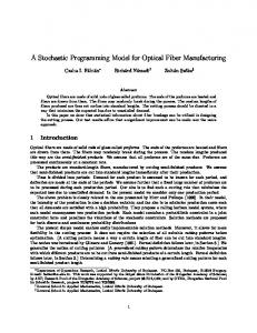
The RLND problem discussed in this paper is an open loop, multi-echelon, multi-product, capacity constraint under return quantity and quality uncertainties. We have developed a SPM to determine the number of collection centers, recycling centers in order to minimize the total cost. The proposed model is including collection points, inspection centers, recycling centers, refinery centers, raw material markets and disposal centers. As shown in figure 1, returned products are collected from customer zones in collection center where is in electronic markets, municipality etc., then they are sent to inspection centers; it is divided into recoverable products and scrapped products. The recoverable products are transported to the recycling centers and scrapped products are sent to the disposal centers.


Figure 1. Proposed reverse logistic network for WEEE

3.1

Stochastic programming

Sahinidis [31] categorizes and reviews the main optimization approaches under uncertainty into three groups: stochastic programming, fuzzy programming, and stochastic dynamic programming. SP is a framework for modeling optimization problems that involve uncertainty [32]. In SP, it is assumed that the probability distribution functions of the uncertain parameters are known and that decision makers try to obtain an optimal solution that minimizes the expected value of objective [33]. The most widely applied SP models are two-stage linear and mixed integer linear programs. A twostage SPM Birge and Louveaux is proposed to take into account randomness. It is developed for a single period context, such as a year [18]. The first stage variables are those that have to be decided before the actual realization of the uncertain parameters becomes available. Subsequently, once the random events have presented themselves, further design or operational policy improvements can be made by selecting, at a certain cost, the values of the second stage or recourse variables. The objective is to choose the first stage variables in a way that the sum of first stage costs and the expected value of the random second stage or recourse costs is minimized. Some notable applications of SP include scheduling, facility location, vehicle routing, and process scheduling [32]. In this contribution, the first stage of the model deals with the location of inspection and recycling processing centers, and the assignment of collection points to inspection centers. The second stage deals with the tactical decisions of the quantity of product flows between centers. The second stage decisions depend on the first stage decision variables y, and on a scenario θ ∈Ω of the random parameters for a given network-operating context. Random parameters relate to quantity and quality of returns. Let Ω be the set of all possible scenarios and θ a particular scenario. Also, let all binary variables be included in vector y and all the continuous variables in vector x. Let f be the vector of the fixed costs related to the opening of the facilities and c the vector containing the remaining coefficients in the objective function. For a



particular scenario the compact model can be stated as follows: Min fy +cθx s.t. Ax ≥ dθ Nθx = 0 Mx ≤ 0 Bx ≥ Cy y ∈ {0, 1} , x ∈ R+. If πθ denotes the probability of scenario θ, then because θ is a finite number of discrete scenarios the expected value function becomes a summation on θ and the uncertain model for compact form can be formulated as the following MILP model [34]: Min

fy+

∑θ π θ .cθ .xθ

s.t. Axθ ≥ dθ Nθxθ = 0 Mxθ ≤ 0 Bxθ ≥ Cy y ∈ {0, 1} , xθ ∈ R+ Note that the obtained solution for this model is not optimal for individual scenarios, but it gives the network structure for the worst possible scenario. For further details, please refer to the work of [34]. Assumptions: The proposed model considers the following assumptions: • All of the returned products from customers of the recycling firm are collected. • Inventory costs are ignored. • Proposed model is based on a single period of time. • There is not any safety stock in collection, inspection and recycling centers. • There are capacity constraints of collection, inspection, and recycling centers. • All costs and allocation rates of products and materials are known. • Locations, capacities and numbers of collection, inspection, recycling and disposal centers are known in advance. • Transportation costs of full trucks are considered and same at each route. According to above descriptions, the SPM under uncertainties quantity and quality can be defined as follows.

3.2

Proposed Two Stage Programming Model

Stochastic

The aim of the RLND is to determine the location of collection, inspection and recycling centers, and to find the quantity of flow between the network

facilities. The presented model includes the following sets, parameters and decision variables: Indices i:Index of collection center locations i∈I={1,..,Ni} j:Index of inspection center locations j∈J={1,..,Nj} k:Index of recycling center locations k∈K={1,..,Nk} b:Index of disposal center locations b∈B={1,..,Nb} r: Index of refinery center locations r ∈R={1,..,Nr} h:Index of material supplier locations h∈H={1,..,Nh} p: Product p∈P={1,…,Np} m: Material m∈M={1,…,Nm} s: Scenario s∈S={1,…,Ns} Parameters ei:Annualized fixed costs for opening potential collection center i fj:Annualized fixed costs for opening cost of potential inspection center j gk:Annualized fixed costs for opening cost of potential recycling center k tcipij:Unit transportation cost for product p from collection center i to inspection center j tirpjk:Unit transportation cost for product p from inspection center j to recycling center k tidpjb:Unit transportation cost for product p from inspection center j to disposal center b trrpkr:Unit transportation cost for product p from recycling center k to refinery center r trmmkh:Unit transportation cost for material m from recycling center k to material supplier h trdpkb:Unit transportation cost for product p from recycling center k to disposal center b ccpi:Unit collection cost for product p at collection center c icpk:Unit inspection cost for product p at inspection center j rcpk:Unit processing cost for product p at recycling center k dcpb:Unit disposal cost for product p at disposal center AC :Advertisement cost CICj:Annual capacity of inspection center j (ton) CRCk:Annual capacity of recycling center k (ton) dciij:Distance between collection location i and inspection center j (km) dirjk:Distance between inspection center j and recycling center k (km) didjb:Distance between inspection center j and disposal center b (km) drdkb:Distance between recycling center k and disposal center b (km) drmkh: Distance between recycling center k and material supplier h (km) drrkr:Distance between recycling center k and refinery center r (km) Sci: Minimum number of collecting center Scj :Minimum number of inspection center Sck: Minimum number of recycling center βm:Rate of product sent from recycling center k to material supplier s



γp:Rate of materials sent from recycling center k to disposal center b δp:Rate of materials sent from recycling center k to refinery r rips:Annually total returned p product to collection points in scenario s a1:Rate of product sent from inspection center j to recycling center k πs:Probability of scenario s Decision variables X cipijs :Product p flow from collection center i to inspection center j in scenario s X irpjks :Product p flow from inspection center j to recycling center k in scenario s X idpjbs :Product p flow from inspection center j to disposal center b in scenario s rr X pkrs :Product p flow from recycling center k to refinery center r in scenario s rm X mkhs : Material m flow from recycling center k to material supplier h in scenario s rd X pkbs : Product p flow from recycling center k to disposal center b in scenario s Wi: Indicator opening j. collection center [0, 1] Yj: Indicator opening j. inspection center [0, 1] Zk: Indicator opening k. recycling center [0, 1] Vij: Indicator of connecting collection center i to inspection center j In terms of the above-mentioned notations, the multi-product multi-echelon stochastic reverse logistic network design problem can be formulated as follows: Objective: Total Cost Minimization ∑Wi ei + ∑ Y j f j + ∑ Z k g k (Facility fixed opening i

j

k

cost)+ π s [∑ p ∑ i ∑ j ∑ s X cipijs .tci pij .dciij +

∑ ∑ ∑ ∑ ∑

p

p

p

m p

∑ ∑ ∑ ∑ ∑

j

j

k

k k

∑ ∑ ∑ ∑ ∑

k

b

r

h b

∑ ∑ ∑ ∑ ∑

s

X irpjks .tirpjk .dirjk +

s

X idpjbs .tid pjb .did jb +

s

X

rr pkrs

.trrpkr .drrkr +

s

rm X mkhs .trmmkh .drmkh +

s

rd X pkbs .trd pkb .drd kb ]

(transportation cost) +

∑ ∑ ∑ ∑ ∑

p

p

p

p

p

∑∑ ∑ X ∑∑ ∑ X ∑∑∑X ∑∑∑X ∑∑∑X i

j

s

ci pijs

.cc pi (collecting cost) +

i

j

s

ci pijs

.ic pi (inspection cost) +

j

k

s

ir pjks

.rc pk (recycling cost) +

j

b

s

id pjbs

.dc pb +

k

b

s

rd pkbs

.dc pb (disposal cost) (1)

Constraints Flow Constraints

ci X pijs = rpsi .Vij (∀ p∈P, ∀ i∈Đ, ∀ j∈J, ∀ s∈S)

∑X

ir pjks

=∑ X

k

ci pijs

(2)

.a p

i

(∀ p∈P, ∀ k∈K, ∀ s∈S) ∑ X idpjbs =∑ X cipijs .(1 − a p ) b

(3)

i

(∀ p∈P, ∀ j∈J, ∀ s∈S) rm ir =∑∑ X pjks .R pm .β m ∑ X mkhs h

j

p

(∀ m∈M, ∀ k∈K, ∀ s∈S) rd =∑ X irpjks .γ p ∑ X pkbs b

(4)

(5)

j

(∀ p∈P, ∀ k∈K, ∀ s∈S) rr =∑ X irpjks .δ p ∑ X pkrs r

(6)

j

(∀ p∈P, ∀ k∈K, ∀ s∈S) Capacity Constraints ci =KOM jp .Y j ∑ X pijs

(7)

i

(∀ p∈P, ∀ j∈J, ∀ s∈S) ∑ X irpjks =KGDM kp .Zk

(8)

j

(∀ p∈P, ∀ k∈K, ∀ s∈S) Logic Constraint ∑Vij =1 (∀ i∈Đ)

(9) (10)

j

Facility Number Constraints ∑Wi =Sci

(11)

i

=Si j

∑Y

i

(12)

j

∑Z

k

=Srk

(13)

k

Integer and Non-negative Constraint ci rr rd rm X pijs , X irpjks , X idpjbs , X pkrs , X mkhs , X pkbs ≥ 0 and

Wi, Yj, Zk, Vij∈ (0,1)

4.

(14)

Application

The RLND problem discussed in this paper is an open loop, multi-echelon, multi-product, capacity constraint under return quantity and quality uncertainties. We have developed a SPM to determine the number of collection centers, recycling centers in order to minimize the total cost. The proposed model is including twenty eight collection points, where is located some city in Turkey, seven inspection centers (j1:Đzmit, j2:Tekirdağ, j3:Erzurum, j4:Antalya, j5:Kayseri, j6:Diyarbakır and j7:Zonguldak), five recycling centers (i1:Đzmit, i2:Ankara, i3:Đzmir, i4:Adana and i5:Samsun), a refinery center and two disposal centers. As shown in table 1, returned products are collected from customer zones in collection center where is in electronic markets, municipality etc., then they are sent to inspection centers; it is divided



into recoverable products and scrapped products. The recoverable products are transported to the recycling centers and scrapped products are sent to the disposal centers. In our study, it is difficult to predict the amount of returned products because of uncertainty. In the next chapter, we address how to handle uncertainty during RLND. Table 1. RL Network Structure RL Structure Products Collecting Points Inspection Centers Recycling Centers Disposal Centers Refinery Centers Raw material markets

Number 4 28 7 5 2 1 2

5. Computational Results

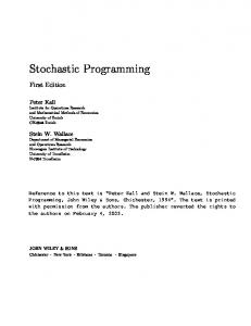
Figure 2. Facility locations for stochastic model

In this section, a numerical example is presented for the proposed model. In order to assess the performance of the proposed SPM, once a deterministic model is developed. In this section, both deterministic and SPM are solved in Windows 7 Centrino Duo 1.86 GHz computer with 512 MB RAM. The Proposed SPM is solved by commercial software GAMS 21.6/CPLEX 6.0. The deterministic solution is derived by using the mean value of each stochastic parameter at eighteen scenarios. The results are presented in Table 2. According to Table 2, runs of deterministic model were done within 0.047 seconds. Compared to deterministic model, runs of stochastic model were done within 0.234 seconds. Deterministic model running time is lower than SPM because of the complexity of stochastic model. Table 2. Summary of the models

Objective Function CPU Time Number of Iterations Single Equations Single Variables Discrete Variables

1.771.913, 5 TL) is higher than total cost of the SPM (1.691.779, 5 TL). Therefore, it can be concluded that results of the SPM propose more economical and compromised solution. According to the results of deterministic model and SPM, all collection centers except Diyarbakir are chosen as inspection centers and also Izmit and Ankara are chosen as recycling centers shown as in figure 2.

Deterministic Model

Stochastic Model

1.771.913,5 TL

1.691.779,5 TL

0.047 sec

0.234 sec

77

473

985

17,186

1,302

19,407

236

236

The deterministic model is developed by using the mean value of eighteen scenarios. As it can be seen at Table 2, total cost of deterministic model

It can be clearly seen from the results that Izmit and Ankara are the best alternatives for the RL network of the recycling firm. It is not suitable to open recycling centers in Đzmir, Adana and Samsun. All collection centers except Diyarbakır are chosen by both of deterministic and SP model as inspection centers. This solution is also supported by historical data related to product returns quantity from customers. Generally the choices are meaningful because of chosen location for inspection and recycling centers are nearer to the industrial zones this will cause a decrease in transportation cost and response time. To compare the optimal solutions obtained by SP with the results of the deterministic approach, a quality criterion, the gap of solution or the relative value of the stochastic solution (RVSS) is defined according to the following equation [41] and [42]: Stochastic-Deterrministic (15) RVSS= Deterministic

According to the solution of RVSS = 4,5%, so SP is more efficient and economical than deterministic model. Then the optimal variables of deterministic approach are considered as an input for two-stage model and it is allowed that second-stage decisions to be chosen optimality as functions of deterministic solution. Therefore, we obtain stochastic solution (b). By using this solution, the relative value of the stochastic solution (RVSS) is 3,36 %. In conclusion SP ensures lower total cost than deterministic model.

5.1

The validation of proposed SPM


A general question in the stochastic programming is whether this approach can be nearly optimal. The theoretical answer to this question is provided by two concepts: the expected value of perfect information (EVPI) and the value of stochastic solution (VSS). EVPI measures the maximum value a decision maker would be ready to pay in return for complete (and accurate) information about the future. The EVPI is difference between the wait-and-see solution (WS) approach and the stochastic programming. In the WS approach, each scenario separately is solved and the mean of objective functions is considered as wait-and-see solution. In this study, the mean of objective functions are calculated as WS= 1.766.299, 15 TL. The expected value of perfect information is, by definition, the difference between the wait-and-see and the here-and-now solution, namely, EVPI = RP−WS (16) EVPI= SP – WS = -74.519, 65 TL To compute the VSS, first the mean value of each stochastic parameter is taken and the model is solved by mean of each parameter, known in the literature as Expected Value (EV) approach. Then the optimal variables of EV approach are considered as an input for two-stage model and it is allowed that second-stage decisions to be chosen optimality as functions of EV solution and stochastic parameters, known in the literature as EEV approach. The difference between the objective functions of EEV approach and stochastic program would be VSS. VSS= EEV - SP (17) VSS = 20.595,06 TL. This quantity is the cost of ignoring uncertainty in choosing a decision. The results show the values of stochastic program is less than WS problem as expected that it lead to the negative values for EVPI measure. In addition, the computation shows that the solution of EEV approach is feasible. This issue points that solution of EV approach in terms of two-stage stochastic program (RP problem) is a good solution and covering the solution of RP problem. These reports confirm the accurateness of two-stage stochastic program and give the consistent results for the presented model.

5.2


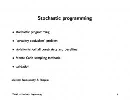
Figure 3. Relation between the total cost and return quantity.

Figure 3 shows the relation between the total cost and return quantity. As illustrated in Figure 3, it is obvious that an increasing in return quantity increases the total cost for both of the models. It should be noted that the cost of the reverse network is directly depended on the quantity of returned products. As can be seen that the capacity of the existing facilities is not sufficient to satisfy the returns for some return quantity; therefore new facilities should be opened and the corresponding fixed cost elevates the total cost value. For instance, when return quantity increase 150%, new inspection center should be open in order to satisfy the returns. Therefore, due to new inspection center opening, total cost increase as seen on the figure in terms of return quantity over 150%. In conclusion, return quantity affects total cost positively both of two models. According to Figure 4, it is obvious that an increasing in quality ratio increases the total cost for both of the models. Quality ratio in this study is associated with the sorting ratio of return products. This ratio can vary due to return products qualities. Figure 6 shows the effect of sorting ratio on the total cost. It can be seen clearly, there is positive linear relationship between sorting ratio and total cost for both of two models.

Sensitivity analysis

In this section, it is tested the performance of the proposed model in several cases by changing some of the parameters. A sensitivity analysis is required in order to find the parameter effects on the results. In this contribution, we conducted some sensitivity analysis on return quantity, quality ratio, variable costs, and collection cost to investigate the effects of these parameters on the objective values.

Figure 4. Relation between the total cost and quality ratio.


Figure 5. Relation between the total cost and variable cost

Figure 5 illustrates that an increasing at the variable cost, which includes transportation costs and operational costs, increases total cost for both of the models. As the Figure 5 shows the total cost of the SP is less significantly sensitive than deterministic model. Also the results show that total cost increase with a linear pattern.

Figure 6. Relation between the total cost and collection cost

According to figure 6, it is obvious to increase in collection cost affects the total cost positively for both models. As can be seen in the Figure 6, the results show that the relation between total cost and collection cost is positive linear.

6.

Conclusion

Due to economic, political, and environmental reasons factors more and more companies are engaged in the product recovery business. Recovery options involve repair, remanufacturing, and recycling. Uncertainties in term of return product quantity, quality and time are the main characteristic of RL networks. Although factors are not always certain in the real world, deterministic modeling assumes factors as certain. The methods that cope with uncertainty help researchers to find more realistic solutions. SPM is generally preferred approach in dealing with uncertainty. This paper presents a two stage SPM under quantity and quality uncertainties in RLND as a real world case study of waste of electric and the waste of electrical and electronic equipment recycling firm to minimize total cost. The RL


network is considered as an open-loop reverse logistics network including collection points, inspection centers, recycling centers, disposal centers, and refinery center. The behavior of this model has been studied when some of parameters such as return quantity and sorting rates are uncertain described by a finite number of the possible scenarios generated via historical data. To cope with product return uncertainty, six scenarios generated from discrete exponential distribution, which is obtained by historical product return data for all collection centers. Probabilities of all scenarios are assigned to each scenario in order not to emphasize any of the scenarios. Second uncertainty is return product quality. Return quality is associated with sorting ratio. To cope with quality uncertainty three scenarios is generated. Therefore for handling quantity and quality uncertainties, eighteen scenarios are generated. Computational results show that the SPM gives more economical and efficient solutions compared to deterministic model. SPM is more successful than deterministic model to handle uncertain parameters. The validation of the solution and sensitivity analyses of the proposed model is conducted. This allows planning maker to take a better decision and to understand how the system behaves under different rate of returns, collection cost, quality ratio, and variable cost. In this paper, the presented model can help managers to handle quantity and quality uncertainties in process of strategic decision making on facility location allocation. This study contributed to literature by handling return quantity and quality, which is related to sorting ratio in inspection centers, uncertainties at the same time in RLND. Second contribution is that we presented a generic multi-product, multistage recycling network for third party RL firm. Several extensions of this model may be considered for future directions. For instance, other uncertainties such as time, capacity, and transportation cost uncertainties can be addressed. Heuristic methods can be developed to increase computational performance quality. Moreover, approximations and sampling-based of the solution approach may be considered for addressing very large number of scenarios.

References [1]

[2]

Lee, D., & Dong, M., “Dynamic network design for reverse logistics operations under uncertainty”, Transportation Research Part E: Logistics and Transportation Review, vol. 45, no. 1, pp. 61–71, Jan. 2009. Lee, J.-E., Gen, M., & Rhee, K.-G., “Network model and optimization of reverse logistics by hybrid genetic algorithm”, Computers & Industrial


[3]

[4]

[5]

[6]

[7]

[8]

[9]

[10]

[11]

[12]

[13]

[14]

Engineering, vol. 56, no. 3, pp. 951–964, Apr. 2009. Yongsheng, Z., & Shouyang, W., “Generic model of reverse logistics network design”, Systems Engineering, vol. 8, no. 3, 2008. Srivastava, S., “Network design for reverse logistics”, Omega, vol. 36, no. 4, pp. 535– 548, Aug. 2008. Sasikumar, P., Kannan, G., & Haq, A. N., “A multi-echelon reverse logistics network design for product recovery—a case of truck tire remanufacturing”, The International Journal of Advanced Manufacturing Technology, vol. 49, no. 9– 12, pp. 1223–1234, Mar. 2010. Fleischmann, M., Krikke, H.R., Dekker, R., & Flapper, S.D.P., “A characterisation of logistics networks for product recovery”, Omega, vol. 28, no. 6, pp. 653–666, Dec. 2000. De Brito, M.P., Dekker, R., & Flapper, S.D.P., “Reverse Logistics : a review of case studies”, ERIM Report Series Reference No. ERS-2003-012-LIS, available at: http://ssrn.com/abstract=411649 . Last access:11.08.2014. Du, F., & Evans, G., “A bi-objective reverse logistics network analysis for postsale service”, Computers & Operations Research, vol. 35, pp. 2617–2634, Jan. 2007. Srivastava, S. K., “Value recovery network design for product returns” , International Journal of Physical Distribution & Logistics Management, vol. 38, no. 4, pp. 311–331, 2008. Chanintrakul, P., Mondragon, A.E.C., Lalwani, C. & Wong, C.Y., “Reverse logistics network design : a state-of-the-art literature review”, Business, vol. 1, no. 1, 2009. Barros, A. I., Dekker, R., & Scholten, V., “A two-level network for recycling sand: A case study”, European Journal of Operational Research, vol. 110, no. 2, pp. 199–214, Oct. 1998. Krikke, H.R., van Harten, A., & Schuur, P.C., "Reverse logistic network re-design for copiers", OR Spektrum, 21, 381-409, 1999. Jayaraman, V., “The design of reverse distribution networks: Models and solution procedures”, European Journal of Operational Research, vol. 150, no. 1, pp. 128–149, Oct. 2003. Min, H., Jeungko, H., & Seongko, C., “A genetic algorithm approach to developing the multi-echelon reverse logistics network for product returns”, Omega, vol. 34, no. 1, pp. 56–69, Jan. 2006.


[15]

[16]

[17]

[18]

[19]

[20]

[21]

[22]

[23]

[24]

[25]

[26]

Lu, Z., & Bostel, N., “A facility location model for logistics systems including reverse flows: The case of remanufacturing activities”, Computers & Operations Research, vol. 34, no. 2, pp. 299–323, Feb. 2007. Salema, M., Barbosapovoa, A., & Novais, A., “An optimization model for the design of a capacitated multi-product reverse logistics network with uncertainty”, European Journal of Operational Research, vol. 179, no. 3, pp. 1063–1077, Jun. 2007. Kumar, R., Vrat, P., & Kumar, P., “A goal programming model for paper recycling system”, Omega, vol. 36, pp. 405–417, 2008. Chouinard, M., Damours, S., & Aitkadi, D., “A stochastic programming approach for designing supply loops”, International Journal of Production Economics, vol. 113, no. 2, pp. 657–677, Jun. 2008. Ilgin, M.A., & Gupta, S.M., “Environmentally conscious manufacturing and product recovery (ECMPRO): A review of the state of the art”, Journal of Environmental Management, vol. 91, no. 3, pp. 563–91, 2010. Pishvaee, M.S., Rabbani, M., & Torabi, S. A., “A robust optimization approach to closed-loop supply chain network design under uncertainty”, Applied Mathematical Modelling, vol. 35, no. 2, pp. 637–649, Feb. 2011. Qin, Z., & Ji, X., “Logistics network design for product recovery in fuzzy environment”, European Journal of Operational Research, vol. 202, no. 2, pp. 479–490, Apr. 2010. Lee, Y.J., “Integrated forward-reverse logıstıcs system design: An empirical ınvestigation”, PhD thesis, Washington State University, 2009. Listeş, O., “A stochastic approach to a case study for product recovery network design”, European Journal of Operational Research, vol. 160, no. 1, pp. 268–287, Jan. 2005. Listeş, O., “A decomposition approach to a stochastic model for supply-and-return network design”, Erasmus, no. 2000, pp. 1– 27, 2002. Listeş, O., “A generic stochastic model for supply-and-return network design”, Computers & Operations Research, vol. 34, no. 2, pp. 417–442, Feb. 2007. Fonseca, M.C., García-Sánchez, Á., Ortega-Mier, M., & Saldanha-da-Gama, F., “A stochastic bi-objective location model for strategic reverse logistics”, Top, vol. 18, no. 1, pp. 158–184, Jul. 2009.


[27]

[28]

[29]

[30]

[31]

[32]

[33]

[34]

[35]

[36]

El-Sayed, M., Afia, N., & El-Kharbotly, A., “A stochastic model for forward–reverse logistics network design under risk”, Computers & Industrial Engineering, vol. 58, no. 3, pp. 423–431, Apr. 2010. Kara, S.S., & Onut, S., “A stochastic optimization approach for paper recycling reverse logistics network design under uncertainty”, Int. J. Environ. Sci. Tech., vol. 7, no. 4, pp. 717–730, 2010. Gomes, M.I., Barbosa-Povoa, A.P., & Novais, A.Q., “Modelling a recovery network for WEEE: a case study in Portugal”, Waste management, vol. 31, no. 7, pp. 1645–60, Jul. 2011. Amin, S. H., & Zhang, G., “An integrated model for closed-loop supply chain configuration and supplier selection: Multi-objective approach”, Expert Systems with Applications, vol. 39, no. 8, pp. 6782– 6791, Jun. 2012. Sahinidis, N.V., “Optimization under uncertainty: state-of-the-art and opportunities”, Computers & Chemical Engineering, vol. 28, no. 6–7, pp. 971–983, Jun. 2004. Bidhandi, H.M., & Yusuff, R.M., “Integrated supply chain planning under uncertainty using an improved stochastic approach”, Applied Mathematical Modelling, vol. 35, no. 6, pp. 2618–2630, Jun 2011. Hosseini, S., & Dullaert, W., "Robust optimization of uncertain logistics networks", In Farahani, R.Z., Rezapour, S., & Kardar, L. (Eds.), "Logistics operations and management", Elsevier, 2011. Birge, J.R., & Louveaux, F., “Introduction to Stochastic Programming”, New York: Springer-Verlag,1997. Guide Jr.,V.D.R., & Van Wassenhove, L.N., “The evolution of closed-loop supply chain research", Working Paper, Operations Research, Vol. 57, Issue 1, pp. 10–18, 2009. Tibben-Lembke, R.S., & Rogers, D.S., “Differences between forward and reverse logistics in a retail environment”, Supply


[37]

[38]

[39]

[40]

[41]

[42]

Chain Management: An International Journal, vol. 7, no. 5, pp. 271–282, 2002. Tan, A.W.K., & Kumar, A., “A decisionmaking model for reverse logistics in the computer industry”, The International Journal of Logistics Management, vol. 17, no. 3, pp. 331–354, 2006. Pokharel, S., & Mutha, A., “Perspectives in reverse logistics: A review”, Resources, Conservation and Recycling, vol. 53, no. 4, pp. 175–182, Feb. 2009. Rahman, S., & Subramanian, N., “Factors for implementing end-of-life computer recycling operations in reverse supply chains”, International Journal of Production Economics, vol. 140, no. 1, pp. 239–248, Nov. 2012. Pishvaee, M.S., Jolai, F., & Razmi, J., “A stochastic optimization model for integrated forward/reverse logistics network design”, Journal of Manufacturing Systems, vol. 28, no. 4, pp. 107–114, Dec. 2009. Pishvaee, M. S., Kianfar, K., & Karimi, B., “Reverse logistics network design using simulated annealing”, The International Journal of Advanced Manufacturing Technology, vol. 47, no. 1–4, pp. 269–281, Jul. 2009. Alumur, S.A., Nickel, S., Saldanha-daGama, F., & Verter, V., “Multi-period reverse logistics network design”, European Journal of Operational Research, vol. 220, no. 1, pp. 67–78, Jul. 2012.