1. Protection Level Calculation Using. Measurement Residuals: Theory and Results. Juan Blanch, Todd ... statistics: all errors are characterized by a zero mean ... nominal error bounds by more than 50%. ... have enough data points to have a good representation of ... In this formula, the standard deviations of the mixture are.
Protection Level Calculation Using Measurement Residuals: Theory and Results Juan Blanch, Todd Walter, Per Enge Stanford University
ABSTRACT In safety-of-life applications of satellite navigation, the Protection Level (PL) equation translates what is known about the pseudorange errors into a reliable limit on the positioning error. The current PL equations for Satellite based augmentation systems are based on Gaussian statistics: all errors are characterized by a zero mean Gaussian distribution which is an upper bound of the true distribution in a certain sense. This approach is very practical: the calculations are simple and the receiver computing load is small. However, when the true distributions are far from Gaussian, such characterization forces an inflation of the protection levels that damages performance. This happens in particular with error with heavy tail distributions or errors for which there is not enough data to evaluate the distribution density up to small quantiles. Because the computing power is expected to increase at the receiver level, it is worthwhile exploring new ways of computing integrity error bounds. We present a way of computing the optimal protection level when the pseudorange errors are characterized by a mixture of Gaussian modes. First, we show that this error characterization adds a new flexibility and helps account for heavy tails without losing the benefit of tight core distributions. Then, we state the positioning problem using a Bayesian approach. Finally, we apply this method to protection level calculations for the Wide Area Augmentation System (WAAS) using real data from WAAS receivers. The results are very promising: Vertical Protection Levels are reduced by 50% without damaging integrity.
INTRODUCTION In the next ten years the number of pseudorange sources for satellite navigation and their quality is expected to increase dramatically: The United States is going to add two new civil frequencies (L5 and L2C) in the modernized GPS, and Europe is planning to launch Galileo which should be fully operative before 2015, also with multiple frequencies. By combining two frequencies, users will be able to remove the ionospheric
delay which is currently the largest error, thus reducing nominal error bounds by more than 50%. In particular, safety-of-life applications using augmentation systems will be greatly enhanced. However, it will remain a challenge to provide small hard error bounds - Protection Levels – to meet stringent navigation requirements. Airborne multipath, ephemeris error, loss of signal due to scintillation (in equatorial regions), are still a challenge in the path to provide Cat III GNSS augmentation systems. For example, even with dual frequency, it is not obvious that the Wide Area Augmentation System (WAAS) with GPS alone would meet 100% APV II (20 meters vertical) availability over the United States [1]. There are many ways to improve the performance of an SBAS without changing the message standards [2]: by adding satellites, by adding reference stations, by improving the algorithms at the master station (specially the clock and ephemeris algorithms). It is worthwhile however, now that the new L5 MOPS is being developed, to explore possible modifications to the message content to improve performance. The current methodologies to provide integrity to augmentation system users are based on Gaussian overbounding techniques. For every source of error, the user receives a standard deviation that corresponds to the Gaussian overbound of the error. For this reason, every source of pseudorange error needs to be overbound, in a certain sense, by a gaussian distribution up to very small quantiles - on the order of the probability of hazardously misdetection (10-7) [3] This is a very difficult task: for example, it is not possible to have experimental stationary distributions for the errors because the conditions and environment are always changing. Also, the errors are all mixed together so it is hard to isolate them. As a result, it is necessary to increase the Gaussian overbound to be sure to cover the tails of the individual error distributions. However, by doing so, we ignore the fact that the core of the distribution is usually much tighter than the overbound (by a large factor), thus giving up performance [4], [5]. In this paper, we present an estimation technique where errors are characterized by Gaussian mixtures. By using a bayesian approach, this technique optimally takes advantage of the tight core of the error distributions while
1
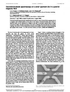
PSEUDORANGE ERROR MODEL Typically, pseudorange errors look Gaussian at the core of the distribution. At the tails, however, either we do not have enough data points to have a good representation of the distribution, or the points that we have suggest that the tails are worse than Gaussian [6]. To illustrate this point, we used data collected at a WAAS receiver in a surveyed position during 6 days, which made it possible to estimate the pseudorange error for each line of sight (there were 4.3x10⁶ samples). Figure 1 shows the quantile-quantile plot (qq-plot) of estimated range errors normalized by the WAAS sigma error. For several probabilities, the quantile of the sample distribution (of normalized errors) is plotted as a function of the corresponding normal Gaussian quantile. This way of plotting the sample was chosen because it provides a visual and practical way of inspecting the relevant characteristics of the sample. In a qq-plot: -
obtained through analysis and following a worst case methodology, that forces the tails of the distribution to be very far. We see that with the Gaussian overbound approach, this uncertainty on the tails of the distribution forces the overbound to be extremely conservative in the core of the distribution.
2 Quantiles of input sample
accounting for the heavy tails. Although this technique could be used in several places at the master station level in an SBAS, or more generally to any estimation problem with heavy tail errors, we will focus on its application to the Protection Level calculation at the receiver. The paper is organized as follows. First, we will explain how the pseudorange error can be characterized by a mixture of Gaussian distributions to account for heavy tails while preserving a tight core. Then, we will compute the a posteriori error density and the resulting error bound on the user position. Finally, we will present a possible application to Protection Level calculation and show its results on real data collected by a WAAS receiver.
Gaussian Overbound
1
Empirical Distribution
0 -1
Gaussian Mixture Overbound
-2 -6
-4
-2
0
2
4
6
Standard normal quantiles
Figure 1. Quantile-quantile plot of normalized pseudorange errors One way to describe the error distribution more accurately is by using a mixture of Gaussian modes. A combination of two Gaussian distributions allows us to account both for the tight core of the distribution and the heavy tails. The density of the error distribution for the Gaussian overbound can then be written, if z is the random variable representing the pseudorange error: p ( zi ) = p0,σ i ( zi )
a sample distributed according to a Gaussian will be represented by a straight line whose slope is the standard deviation of the sample a distribution overbounding the sample distribution in the sense of [3] will appear to be above the curve corresponding to the sample for positive values, and below for negative values
where the indexes represent the mean and the standard deviation. The index i refers to a given line of sight. The idea is to split this distribution in a mixture of two Gaussians:
In this plot, there are several interesting characteristics. First, the unit Gaussian appears to be a conservative overbound of the sample distribution, which is a proof that WAAS is correctly bounding the pseudorange errors. Second, the sample distribution appears to be well described by a Gaussian distribution between the quantiles -3.5 to 3.5 approximately, which corresponds to a probability of 10-4. Third, we can see how the tails of the distribution are not as well behaved as the core of the distribution, although well covered by the Gaussian overbound. We need to keep in mind that the Gaussian overbound is not obtained through inspection of this type of plots. The tails of the distributions are typically
In this formula, the standard deviations of the mixture are defined as a function of the original WAAS standard deviation. For this paper, we determined the three additional parameters arbitrarily but with the following requirements: the resulting distribution had to be an overbound of the sample distribution, and for large quantiles, it had to be an overbound of the original overbounding distribution. With these requirements, we chose: acore = 0.975 γ core = .3
-
p ( zi ) = acore p0,γ coreσ i ( zi ) + atails p0,γ tailσ i
atails = 0.025
γ tails = 1.5
2
The resulting distribution is plotted in Figure 1 as a red line. One can check that all requirements are met and that while we are less conservative at the core of the distribution, the new error distribution is an overbound of the original overbounding distribution in the tails.
POSITION ERROR DISTRIBUTION Now that we have a statistical description of each pseudorange error, in this section we give some elements calculation of the position error distribution, (and leave the rest for the Appendix). In the previous section we have written the density for a single pseudorange. Here we need the density of the vector of errors affecting the vector of pseudoranges. After assuming that the errors are independent, it is shown in the Appendix that the joint distribution is a mixture of multivariate Gaussians. The density of the vector of errors z is given by: p(z) =
N modes
∑ j =1
pi fCi ( z )
This is equivalent to saying that the covariance of z is Ci with probability pi (we assume that the errors are zero mean). All the parameters of this distribution are derived from the individual parameters corresponding to each pseudorange (see Appendix). We also need to specify what is meant by the measurements y. The GPS positioning problem is not linear; however, if one guesses a solution that is close enough to the true solution, the problem is well approximated by a linear model. Here we assume that a position fix has been determined, and x is then the difference between the true position and the determined fix, and y is the vector of residuals. As a consequence we can assume that the linear model for GPS measurement holds (G is the geometry matrix): y = Gx + z
We now evaluate the probability density of the position x given the measurements y. It is rare to consider this expression because, when the errors are Gaussian and a least squares estimator with the proper covariance is used, the error density is given by a multivariate Gaussian centered a the estimated position, whose covariance does not depend on the measurements (one can compute the covariance of the position estimate without knowing the actual measurements). But here the situation is different, as the errors are no longer Gaussian. The calculation is starts with Bayes formula:
p ( x | y) =
p ( x, y )
p ( y | x) p ( x)
=
p( y)
p( y)
Here p(x) designates the a priori distribution of the position, which is here made to tend to a uniform distribution over the whole space, as we assume no a priori information on the position. The expression for
p ( y | x ) is easy to compute, because z is a mixture of
Gaussian distributions: p ( y | x) =
N mod
∑p j =1
j
Wj
1 2
e
−
1 ( y − Gx )T W j ( y − Gx ) 2
where Wj is the inverse of the covariance Cj matrix corresponding to the jth mode: W j = C −j 1
After some algebra (see Appendix) we find that :
p( x | y) =
N mod
∑c j =1
j
p ( j) xˆ
(
, GT W j G
)
( x)
−1
where:
(
j xˆ ( ) = G T W j G
)
−1
GT W j y
and where the coefficients aj are defined by:
cj =
p j Wj N mod
∑p i =1
where:
(
i
1 2
Wi
GT W j G 1 2
−
GT Wi G
1 2 −
e
1 − χ 2j 2
1 2
e
1 − χi2 2
)
χ 2j = yT W j − W j G ( G T W j G ) G T W j y −1
This expression gives the a posteriori distribution of the position location given the measurements. This density appears as a linear combination of Gaussian densities associated with the optimal least square estimate corresponding to each mode. One can see that the expression depends heavily on the measurements themselves through the chi-square statistic for each of the covariances in the mixture, and through each corresponding estimate.
3
POSITION ERROR BOUND CALCULATION
Here we explain how to translate the density in an error bound for a given probability ε. Let us suppose that we want to compute an error bound in the vertical domain. The problem is to find a position estimate xˆ1 and an error bound (the Vertical Protection Level (VPL)) such that:
(
)
Prob x1 − xˆ1 > VPL | y < ε From the density of the position, it is easy to derive the density for each coordinate: p ( x1 | y ) =
N mod
∑a j =1
j
p ( j)
(
xˆ1 , GT W j G
)
−1
( x1 )
1,1
To determine xˆ1 and VPL, we need to find an interval I
To perform this split the user needs three additional scalars: - the probability of being in the core of the distribution acore, - the ratio between the standard deviation of the core and σi (smaller than one) γcore - the ratio between the standard deviation of the tails and σi (smaller than one) γtails The numerical value of these parameters is the one determined in the section Pseudorange Error Model. One could choose to make this parameters depend on the satellite, but it would be also possible to set a conservative set of parameters valid for all satellites, and this is the approach that will be taken here. Such an addition to the MOPS [2] would be backwards compatible: a user without the capability to apply the new algorithm would simply use the current PL equations.
such that:
∫ p(x
1
| y) ≥ 1− ε
x1 ∈I
This interval is not unique and can be adapted to different requirements. In this work we chose to determine it by setting the probability of being on each side of the interval to ε/2. This can be easily implemented using a slicing algorithm (it takes very few iterations) to determine independently each bound. Once we have the upper and the lower bound of the interval it is straightforward to compute a VPL for any chosen estimate.
APPLICATION TO SBAS PROTECTION LEVEL AND MESSAGE CONTENT
As an example and possible application, we suggest here a small modification to the SBAS message content that would allow SBAS users to take advantage of this technique. As indicated in the Introduction, the current SBAS message (defined in the Minimum Operational Performance Standards for SBAS (MOPS)) allows users to compute at each time the standard deviation of each pseudorange error [6] σi2. The user treats the pseudorange error as if it was a Gaussian random variable with zero mean and standard deviation σi2. As explained in the section Pseudorange Error Model, we can account for the fact that the errors have a tight core and heavy tails by splitting this single mode in two modes: one describing the core and another one describing the tails. The random error with density p0,σ 2 ( zi ) is replaced by: i
acore p0,γ coreσ i ( zi ) + (1 − acore ) p0,γ tailsσ i ( zi )
EXPERIMENTAL RESULTS
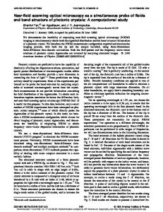
We compared two options to compute the Vertical Protection Level: - Gaussian overbound: the VPL is computed using the current SBAS VPL equation using a model for broadcast sigmas (which leads to the previous histogram) New algorithm: as said before, the pseudorange error distribution is derived from the previous one by splitting the gaussian mode in a mixture of two gaussian modes Using pseudorange data collected over a day by a WAAS receiver at a surveyed location, we computed every 5 s the Vertical Protection Level using both methods. As mentioned in the previous section, it is possible to adjust the estimate in the new method to minimize the VPL. Here we chose to keep the estimate as the one predicted by the current method, and only changing the VPL, so there is only one estimation error reported for each fix. Figure 2 displays a time series of the VPL as well as the error. Figure 3 shows vertical alert limit as a function of unavailability for both methods. Figure 4 and 5 is the triangle chart of the results, where a two dimensional histogram is binned by the true vertical error in the x-axis and the vertical protection level in the y-axis. The VPL is reduced by almost 50% across all availability figures, despite the fact that the tails of the individual pseudorange distributions are heavier than the original Gaussian overbound. The triangle charts are here to show that integrity appears to be preserved (but this is not a surprising result given the very large gap between the VPL and the actual error always recorded under nominal conditions). -
4
Meters
VPL in meters
Current VPL
40 30 20
New VPL
10 0 0
Current VPL
50 40
2
10 30
20
1
10
10
5
10
15
20
0 0
Time in hours
Number of Points per Pixel
50
0
5
10
15
20
25
10
Vertical Error in meters
Figure 2. VPL and vertical error as a function of time
Figure 4. Triangle chart for the current algorithm
New VPL
Current VPL
40
Meters
VPL in meters
50
30 20 10 0 -3 10
New VPL
40 2
10 30
20 10
0 0
10
-2
1
10
-1
10
Unavailability Figure 3. VPL quantile as a function of unavailability
0
10
0
5
10
15
20
25
10
Vertical Error in meters Figure 5. Triangle chart for the new algorithm
The next set of results corresponds to the same data set to which simulated noise has been added. The pseudorange was modified by adding a constant random bias per track. To match the characteristics of the true error, it was generated using a Gaussian mixture. In Figure 6 we can see how the new algorithm reacts to real position errors (between 11 and 12 hours). Figure 7 shows the VAL as a function of unavailability, which has gone down for the new algorithm but is still well below the current algorithm.
5
Number of Points per Pixel
50
40
40
30 20
10
2
10
1
10
0
30 20 10
10 0 0
Current VPL
5
10
15
0 0
20
5
10
15
20
25
Number of Points per Pixel
50
VPL in meters
Meters
50
Vertical Error in meters
Time in hours
Figure 8. Triangle chart for the current algorithm
Figure 6. VPL and vertical error as a function of time
New VPL 50
Meters
VPL in meters
Current VPL
40 30 20
New VPL
10 0 -3 10
40
2
10
30 1
20
10
10 -2
10
-1
10
Unavailability Figure 7. VPL quantile as a function of unavailability
Figures 8 and 9 show the most interesting result of this research: we can see how most of the VPLs have been reduced by more than 50%, but only when it was safe to do so. For large position errors, the VPL remains almost at the same level as before. These plots suggest that the new algorithm offers a means of drastically reducing the Protection Levels without affecting integrity.
0
10
0 0
0
5
10
15
20
25
10
Vertical Error in meters Figure 9. Triangle chart for the new algorithm
COMPUTATIONAL AND INTEGRITY ISSUES
As it has been presented, this algorithm has some theoretical weaknesses: - the theory assumes that errors are independent (although correlation could be introduced, if we knew what the appropriate correlation is) - biases are not accounted (however, very large biases would be detected)
6
Number of Points per Pixel
50
-
using a very spread distribution for the failed mode could cause an underestimation of the error (this risk is small, but that needs to be proved) The two first points are already present in the current overbounding approach, but because of the large margin, they are not a major concern. The last point is specific to the new algorithm and needs to be well understood and accounted for. By looking at the expression for the a posteriori density, one can see that if, for a given set of measurements, we increase the standard deviation of the outer mode the PL will increase, reach a maximum, and decrease again. As a consequence, using a larger sigma for the outer mode is not always a conservative approach (although in the current results, this phenomenon was not observed).
The method was applied to compute positions and protection levels in an actual WAAS receiver. The error bounds appeared to be 50% smaller on average than with the current VPL calculation, without affecting integrity and across all levels of availability. It is therefore worthwhile studying its application in safety of life positioning systems requiring small error bounds like SBAS, GBAS or Galileo – before new message standards are decided.
APPENDIX
Let z be the random variable representing the pseudorange error. The density of z can be written: q
The computational load comes mainly from the large number of matrix inversions. The number of matrix inversions needed for one position fix is not one, like in the current PL equation, but several hundreds or thousands. This is not an issue for a PC: a position fix and PL computation with 10 satellites took .1 s. This was achieved: - by exploiting the fact that one can go from one inverted matrix to another by rank one updates, which are far less demanding than full matrix inversions, - by excluding terms in the density that are known to be small before computing them However, even with these improvements, it will be challenging to apply this algorithm in a certified airborne receiver.
CONCLUSION
We have developed a formula for the a posteriori position distribution when the pseudorange errors are distributed according to a mixture of gaussian modes. This means that we can theoretically compute the position distribution for any kind of pseudorange error distribution well characterized by a finite mixture of gaussian modes. The most remarkable feature of the formula is its dependence on the actual measurements (via the measurement residuals). Before this method can be applied in an actual system it will be necessary to better understand its behavior, as the dependence of the error bounds on the measurements is more complex than in current methods. Also, this method has a larger computational load. Future work will need to address these issues. While systematically evaluating the new approach using WAAS NSTB data we will study the possible integrity issues and behavior under different error models. Also, we will try to simplify the formula as much as possible in order to reduce its complexity and computational load.
p ( z ) = ∑ ai f mi ,σ i ( z ) i =1
In this equation f mi ,σ i ( z ) is the density of a Gaussian with mean mi and standard deviation σi. The only requirements on the coefficients ai are that their sum be one and that the density be positive for all z. From now on the random variable z is a vector. Let us consider n pseudorange sources and label zk the error on each of them (now z is a vector). Each error is characterized by a Gaussian mixture: qk
p ( zk ) = ∑ ai , k f mi ,k ,σ i ,k ( zk ) i =1
The joint density is given by: n n ⎛ qk ⎞ p ( z1 ,..., zn ) = ∏ pk ( zk ) = ∏ ⎜ ∑ ai , k f mi ,k ,σ i ,k ( zk ) ⎟ k =1 k =1 ⎝ i =1 ⎠
If one develops this expression, we see that the joint distribution is a mixture of multivariate Gaussians. The covariance matrices are given by each possible combination of the modes in each pseudorange error. Let us label Cj the covariance for a given mode and pj the probability of that mode. The density of the random variable z is given by: p(z) =
N mod es
∑ j =1
pi f M i ,Ci ( z )
This is equivalent to saying that the covariance of z is Ci with probability pi. Now that we have a characterization of the error, we can derive an estimator adapted to it. We will start by computing the probability density of the position x given the measurements y:
7
p( x | y)
whole space). There is an analytic expression for the integral term:
It is assumed here that the linear model for GPS measurement holds (G is the geometry matrix):
∫e
y = Gx + z
p ( y)
p ( y ) = 2π
1
Wj 2 e
j
−
1 ( y − Gx )T W j ( y − Gx ) 2
p ( y | x) = =
N mod
∑p j =1
e
p ( y ) , we integrate over all possible
j
(
N mod
∑ j =1
p ( y ) = ∫ p ( y | x ) p ( x ) dx e
−
=
∑p j =1
=
j
1 ( y − Gx )T W j ( y − Gx ) 2
∑p
∫e
∫e
1 T − ( y − Gx ) W j ( y − Gx ) 2
p ( x ) dx
j
(
Wj
1⎛ − ⎜ x − GT W j G 2⎝
1 2
)
e
−1
(
1 ⎛ − yT ⎜ W j −W j G GT W j G 2 ⎝
T
⎞ GT W j y ⎟ ⎠
p ( x ) dx
)
−1
j
N mod
∑p j =1
j
Wj
N mod
∑p j =1
)
1 2
−1
e
j
1 2
Wj
1 2
GT W j G
e
−
−
1 2
e
1 − χ 2j 2
)
1 ( y − Gx )T W j ( y − Gx ) 2
(
1 ⎛ − yT ⎜ W j −W j G GT W j G 2 ⎝
T
⎞ GT W j y ⎟ ⎠
p j Wj
1 2
)
−1
⎞ GT W j ⎟ y ⎠
(G W G )⎛⎝⎜ x −(G W G ) T
T
j
GT W j G
(
j xˆ ( ) = G T W j G
⎞ GT W j ⎟ y ⎠
( G W G )⎛⎜⎝ x −( G W G ) T
1 2
−
1 2
j
e
−1
⎞ GT W j y ⎟ ⎠
1 − χ 2j 2
where:
x
N mod j =1
Wj
1 2
−
T
x j =1
N mod
dx
1 1 j j ⎧⎪ 1 − ( x − xˆ ( ) ) ( GT W j G ) ( x − xˆ ( ) ) ⎫ ⎪ GT W j G 2 e 2 ⎨ ⎬ ⎪⎩ 2π ⎭⎪
x
1 2
⎞ GT W j y ⎟ ⎠
−1
Wj
1⎛ − ⎜ x − GT W j G 2⎝
= 2π
positions:
= ∫ ∑ p j Wj
−1
j
Notice that this expression would be chi-square distributed if the measurements followed the jth mode. The numerator can be written (where p(x) is canceled out):
W j = C −j 1
N mod
T
j
(
where Wj is the inverse of the covariance Cj matrix corresponding to the jth mode:
To compute
T
χ 2j = yT W j − W j G ( G T W j G ) G T W j y
because z is a mixture of Gaussian distributions:
j =1
(G W G )⎛⎜⎝ x −( G W G )
where we have:
Here p(x) designates the a priori distribution of the position. The expression for p ( y | x ) is easy to compute,
∑p
T
⎞ GT W j y ⎟ ⎠
The denominator is then:
p ( x, y )
p ( x, y ) = p ( y | x ) p ( x )
N mod
−1
= 2π G T W j G
Now let us develop p ( x, y ) :
p ( y | x) =
)
x
We start by writing Bayes formula: p( x | y) =
(
1⎛ − ⎜ x − GT W j G 2⎝
T
j
−1
⎞ GT W j y ⎟ ⎠
)
−1
GT W j y
is the position estimate using a least squares algorithm assuming that the measurements have the covariance p ( x ) dx
x
Let p(x) tend to a uniform distribution over the whole space in both the numerator and the denominator (it is possible to include an a priori in the position of x, but to be consistent with the assumptions of current methods we make the a priori tend to a uniform distribution over the
W j−1 . We notice now that the term : 1 1 j j ⎫ − ( x − xˆ ( ) ) ( GT W j G ) ( x − xˆ ( ) ) ⎪ ⎪⎧ 1 GT W j G 2 e 2 ⎨ ⎬ ⎪⎩ 2π ⎭⎪ T
j is the density of a multivariate Gaussian centered on xˆ ( )
(
and with covariance GT W j G
)
−1
which we will note:
8
p ( j) xˆ
(
, GT W j G
)
−1
( x)
With these notations, the density of the a posteriori distribution of x is given by: p( x | y) =
N mod
∑c j =1
j
p ( j) xˆ
(
, GT W j G
)
−1
( x)
where the coefficient aj is defined by:
cj =
p j Wj N mod
∑p i =1
i
1 2
Wi
GT W j G 1 2
−
GT Wi G
1 2 −
e 1 2
1 − χ 2j 2
e
1 − χi2 2
This expression gives the a posteriori distribution of the position location given the measurements.
ACKNOWLEDGEMENTS
This work was sponsored by the FAA GPS product team (AND-730).
REFERENCES
[1] T.Walter, P. Enge, P. Reddan. “Modernizing WAAS,” Proceedings of the Institute of Navigation GNSS 2004, Long Beach, CA, 2004. [2] RTCA (2001) Minimum Operational Performance Standards for Global Positioning System/Wide Area Augmentation System airborne equipment, RTCA publication DO-229C. [3] B. DeCleene. “Defining Pseudorange Integrity – Overbounding,” Proceedings of the Institute of Navigation GPS-00. Salt Lake City, UT, 2000. [4] J. Rife, S. Pullen, B. Pervan, P. Enge. “Core overbounding and its implications for LAAS integrity,” Proceedings of the Institute of Navigation GNSS 2004, Long Beach, CA, 2004. [5] J. Lee. “LAAS Position Domain Monitor Analysis and Test Results for CAT II/III Operations,” Proceedings of the Institute of Navigation GNSS 2004, Long Beach, CA, 2004. [6] WAAS PAN report: http://www.nstb.tc.faa.gov/
9