The main objective of the SedAlp project is to develop tools and strategies ..... Overall, plate geophone systems are an appropriate monitoring device to collect a ...
First SedAlp Milestone
WP5 - Action 5.2 Protocol for data collection method in sediment transport
June, 2013
Introduction The main objective of the SedAlp project is to develop tools and strategies for an integrated sediment management. To reach this ambitious goal, it is elementary to understand the behaviour and characteristics of sediment transport. The knowledge about this complex natural process is still limited, therefore field observations and data on sediment transport are needed. Work package 5 (WP5), with the title “Sediment transport monitoring”, basically aims on providing this data to expand the understanding of sediment transport, debris flows and wood transport. Throughout the whole Alpine Region, a lot of different monitoring methods in sediment transport are currently in use. The presented first SedAlp Milestone, with the title “Protocol for data collection method in sediment transport”, aims on ensuring the comparability of the collected monitoring data. Therefore, three standard protocols on bedload transport, debris flow and wood transport monitoring have been developed. These protocols are intended to describe the used monitoring technics and data processing methods. Furthermore, the protocols work also as guidelines to assist in choosing the appropriate monitoring method for supporting prospective monitoring efforts.
Contents
• Part I - Protocol for Bedload Monitoring • Part II - Protocol for Debris-flow Monitoring • Part III - Protocol for Wood Monitoring
Part I Protocol for Bedload Monitoring
WP5 - Action 5.2 Protocols on standardized data collection methods in sediment transport monitoring for transboundary exchange
Lead authors: Johann Aigner, Andrea Kreisler & Helmut Habersack (PP11), Francesco Comiti (PP1) Contributors: Tobias Heckmann, Judith Abel, Florian Haas & Michael Becht (PP6), Frédéric Liébault (PP7), Matteo Cesca & Alessandro Vianello (PP2)
June, 2013
1
Contents 1
Introduction
3
2
Bedload Monitoring Methods
4
2.1
Mobile Basket sampler
5
2.1.1 Large Helley-Smith sampler (LHS)
5
2.1.2 TIWAG sampler
6
2.1.3 Vent sampler
7
2.1.4 BUNTE traps
8
2.1.5 Sampling procedures
10
2.2
Slot traps
12
2.3
Monitored Retention Basin
14
2.4
Geophone plates
19
2.5
Japanese Pipe Hydrophone (Acoustic pipe sensor)
21
2.6
Tracers
22
2.7
Topographic/morphological methods
26
2.7.1 Terrestrial Laser scanning
26
2.7.2 Drone-based aerial imagery
28
2.7.3 Morphological sediment budgets from multitemporal digital elevation models
29
2.7.4 Scour chains
31
3
Suitability of bedload monitoring methods
33
4
Field forms - Bedload Monitoring
36
4.1
Specific Field form
36
4.1.1 Specific Field form - Basket Sampler (interval measurement)
36
4.1.2 Specific Field form - Basket Sampler (cross-section wise measurement)
37
4.1.3 Specific Field form – Bedload Trap
38
2 5
References
39
3
1 Introduction The movement of sediment particles on or close to the riverbed by rolling, sliding or saltation is called bedload transport. Field-derived knowledge data of bedload transport is required to adequately plan flood protection and torrent control systems, waterway management and in general river engineering works. Furthermore, quantification of bedload transport is needed for issues concerning ecosystem dynamics and hydropower management. From relatively low to flood flows, bedload transport features a dramatic spatio-temporal variability and a fairly stochastic behaviour (Habersack et al., 2008). Therefore, field measurements are essential to select, apply and calibrate bedload transport formulas and numerical models. Nonetheless, measuring bedload transport in natural rivers is still a challenging task. Several different methods are currently used for bedload monitoring worldwide. They all have advantages and disadvantages, thus in many instances it is recommended to combine different methods to achieve the desired goals. The integrative monitoring system presented in Habersack et al (2013, in prep.) shows an example in the use of complementary bedload monitoring methods. The following protocol will give an overview about the different bedload monitoring methods, with more details on those deployed within the Project SedAlp. Furthermore, it should assist in choosing the appropriate monitoring method for questions related to the quantification of bedload transport. Bedload monitoring methods can be divided into two groups: •
Direct methods o Suspended basket samplers o Bunte traps o Slot traps/samplers o Monitored retention basins
•
indirect methods o Passive acoustics (geophone plates, Japanese acoustic pipe, hydrophones) o Active acoustic (ADCP) o Tracers (painted, magnetic, PITs…) o Topographic/geomorphological (repeated laser scanning or photogrammetry, scour chains…)
4
2 Bedload Monitoring Methods Table 1 gives an overview over the main parameters of interest in bedload transport and monitoring methods. Table 1 Main parameters and monitoring methods
[kg m-1s-1]
Specific bedload rate Basket sampler (cross-Section wise measurement, repeated measurement), Bedload trap
[kg s-1]
Bedload rate Basket sampler (cross-Section wise measurement) Bedload yield
[kg]
Basket sampler (cross-section wise measurement)
Spatial variability of bedload transport Basket sampler (cross-Section wise measurement), geophone plates, Acoustic pipe sensor Temporal variability of bedload transport Basket sampler (interval measurement), geophone plates, Acoustic pipe sensor [m;m3s-1;Nm-2]
Initiation of motion Basket sampler (repeated measurement), geophone plates, Acoustic pipe sensor, Tracers
Bedload
trap,
Grain size distribution (sieving required) Basket sampler, Bedload trap
Transport path, Transport velocity
[m; m s-1]
Tracers
variation of sediment storage Scour chains, Terrestrial Laser scanning, Aerial Imagery
[m; m³]
5 2.1 Mobile Basket sampler Bedload measurements with basket samplers are one of the oldest and most common methods of bedload monitoring (Mühlhofer, 1933; Helley and Smith, 1971). The concept of basket sampler measurements is relatively simple. A net is fixed on a rectangular metal frame and lowered to the river bed. Bedload material which passes through the frame gets captured in the net. The minimum sediment size which can be sampled is defined by the size of the net holes. The maximum sediment size is limited by the intake width of the sampler. After sampling, the sampled bedload material is dried, weighted and sieved. With the known measuring time and the intake width, the specific (i.e., per unit channel width) bedload transport rate can be calculated. Different river types require different basket samplers due to their characteristic sediment size, transport intensity and hydraulic conditions. Important aspects in the use of basket sampler are the hydraulic efficiency (back pressure) and possible errors arising from an imperfect use of the basket (over- and under-sampling). Over time several different basket samplers have been developed. Scientific publications are treating topics like, the calibration of bedload samplers, sources of error and their effects of the achieved results and analyses of caught bedload material texture (e.g. Emmett, 1980; Gaudet et al., 1994; Vericat et al., 2006; Habersack & Laronne, 2001).
2.1.1 Large Helley-Smith sampler (LHS) One of the most commonly used basket samplers is the Large Helley Smith (LHS) sampler presented by Helley and Smith (1971). It is a pressure difference sampler with an intake width of 0.152 m x 0.152 m. Different mesh sizes of sampler nets are adopted (0.25 mm, 0.5 mm, 1 mm, 2 mm…) depending on the sampling objective and river type. Sources of error and their effects of the achieved results in the use of LHS basket sampler can be found in Vericat et al. (2006). The LHS basket sampler is lowered to the riverbed with a crane (mounted on a trailer or truck), a river cableway or held directly by hand if wading is possible (small streams). Figure 1 and Figure 2 show some examples of the handling of the LHS basket sampler in Dellach/Drau in Austria.
6
Figure 1 Trailer with crane and LHS basket sampler, Dellach/Drau (Aigner, 2013)
Figure 2 LHS basket sampler, Dellach/Drau (Aigner, 2012)
2.1.2 TIWAG sampler The TIWAG basket sampler (Figure 3) was constructed by the Austrian Hydropower company TIWAG for bedload transport measurements in Mountain Rivers. The intake width is 0.5 m x 0.5 m, the metal grid which captures the bedload has a mesh size of 8 mm. The relatively large mesh size is necessary to assure the hydraulic efficiency. A metal pillar defines the exact position of the bedload measurement. During measurements, the sampler is inserted into the metal pillar by a mobile crane and lowered to the riverbed (Figure 4). With this method only interval measurements of bedload transport can be undertaken. When the sampler is positioned behind a geophone plate, the latter can be accurately calibrated.
Figure 3 TIWAG basket sampler behind plate geophones, Lienz/Isel, Austria (Seitz, 2009)
Figure 4 TIWAG sampler lowered by crane Lienz/Isel, Austria (Seitz, 2009)
7 2.1.3 Vent sampler The Vent basket sampler (Figure 6) was constructed by BOKU (Vienna) and can be seen as a crane-suspended Bunte trap (see 2.1.6) having different dimensions. It was built for bedload measurements in mountain streams with intense bedload transport (Habersack et al., 2012). The sampler consists of three parts: a rectangular steel-frame (0.44 m x 0.26 m), a sampler bag with a mesh size of 3.5 mm x 6.5 mm and a vertical steel bar. The steel bar is attached, so that the frame can turn into the flow selfadjusting based on the prevailing direction. The sampler can be mounted on a mobile crane at the shackle at the upper end of the steel bar. To prevent the sampler from moving downstream, two tether lines are fixed at the loops on the sides of the frame and on both riverbanks.
Figure 5 Bedload measurement with the Vent basket sampler and a mobile crane, Vent/Rofenache (Aigner, 2012)
Figure 6 Vent basket sampler (Seitz, 2010)
8 2.1.4 BUNTE traps “Bunte” traps are portable sampler developed to facilitate sampling irregular and infrequent gravel and small cobble over a wide range of transport rates in wadeable mountain streams (Bunte et al., 2004). The development was a joint effort between the Colorado State University (CSU), Engineering Research Center and the USDA Forest Service (FS), Stream System Technology Center. Original “Bunte” traps have a 0.3m x 0.2m aluminum frame as the sampler opening, allowing coarse gravel and small cobble particles to enter the trap. The frame has a trailing net with a 4 mm mesh that stores the collected gravel bedload. The net, typically about 1 m long, can be opened, emptied, and closed from the back. These traps are placed on ground plates anchored to the stream bottom with metal stakes. Adjustable nylon webbing straps are used to fasten the frame to the stakes. Ground plates prevent involuntary particle entrainment at the sampler entrance and ensure that all particles that have moved onto the ground plate will enter the trap (Bunte et al., 2007). Indeed, the correct positioning of ground plates is crucial in ensuring a good performance of these traps, making Bunte traps generally more reliable and accurate than Helley-Smith samplers (used without plates) in gravel bed rivers (Bunte et al., 2008).
Figure 7 Sketch of a Bunte trap (from Bunte et al. 2007)
The combination of large opening, large sampler capacity, installation on ground plates, and long sampling times are essential for obtaining representative samples of gravel and cobble bedload transport. Because these attributes are more typical of a trap than a sampler, the developers
9 used the term “bedload trap”, even though the device is not installed below the bed surface as the slot traps described in the following section. For detailed information on the construction and use of the “Bunte” traps, please refer to Bunte et al. (2007).
Figure 8 Left: Bunte traps can be left unmanned in relatively slow flows (from Bunte et al., 2007). Right: in fast turbulent streams the traps are ensured to be in perfect contact with the ground plate by keeping a foot on the upper side of the frame during the sampling time (Saldur River, Italy).
Recently, Kociuba et al. (2012) developed a variation of the “Bunte” traps where multiple samplers can be operated by a single operator standing on a river bank. For more information on this “River bedload trap”, see http://www.freepatentsonline.com/EP2333161.html. Bunte traps have proven quite effective in determining bedload transport rates and sediment mobility up to bankfull conditions in wadable gravel- and cobble-bed streams (Bunte et al., 2004; Bunte et al., 2010; Dell’Agnese et al., 2012) as well as to calibrate an acoustic pipe sensor installed in a mountain river (Dell’Agnese et al., 2013).
10 2.1.5 Sampling procedures Cross-section measurements More bedload measurements across a river section are necessary both to gain information about the spatial variability of specific bedload transport rate (kg m s-1) and to calculate the total bedload transport rate (kg s-1) through a section. A river cross-section is divided into different verticals based on hydraulic and morphological considerations, which represent the locations where basket sampler is deployed on the bed. The number of measured verticals varies with river width. On one side, the more verticals are measured, the more accurate will be the calculated bedload transport and the better is the knowledge about the spatial variability of bedload transport. On the other hand, hydraulic conditions should not change during the measurement, which limits the number of verticals. Figure 9 shows an example of a cross section measurement at the Drau river in Dellach (Austria) undertaken with a Large Helley Smith basket sampler. To account for temporal variations in bedload transport three measurements per vertical are recommended (Habersack et al., 2008).
Figure 9 Cross section measurement with the Large Helley-Smith Sampler at Dellach/Drau (Habersack et al., 2008).
11 Repeated measurements As mentioned above, bedload transport often shows a strong temporal variability even for constant hydraulic conditions. Repeated measurements at the same vertical are undertaken to capture and quantify such variability. Therefore single basket sampler measurements are repeated at the same vertical over a long period of time. A possible outcome of interval measurements is presented in Figure 10 and shows the temporal variability at a given vertical at Dellach/Drau (Habersack et al., 2008).
Figure 10 repeated measurement with the Large Helley-Smith Sampler at Dellach/Drau (Habersack et al., 2008).
12 2.2 Slot traps This direct bedload monitoring system permits continuous bedload measurements at predefined locations within a cross-section (Reid et al., 1980; Habersack et al., 2010). The slot trap consists of a sample container, covered by a slotted plate and inserted in a formed (concrete) pit in the riverbed. To start bedload sampling the slot is opened (hydraulically via manual control or by hand), enabling bedload material to be trapped into the container. Load cells or a pressure pillow commence recording automatically the mass increase within the trap. To be able to analyse the trapped material a crane withdraws the filled container and places it on to the riverbank. The empty trap has to be reinserted into the riverbed for further measurements. Bedload traps enable continuous and automatic bedload transport measurements and achieve accurate and reliable results. Thereby, the method is applicable for all water stages, especially during floods, when other sampling methods are not operable anymore. Besides, it enables the determination of the complete grain size spectrum. The sampling durations depend on the intensity of bedload transport and is limited by the reservoir capacity of the trap. The measured mass increase by time enables the calculation of the specific bedload transport and further provides an excellent inside in the temporal variability of bedload transport process. Due to its fixed position in the cross-section, the gathered information is spatially limited. This limitation can be reduced by additional measurements with surrogate instruments like plate geophones. Bedload traps are well suited to calibrate the signal of surrogate instruments (geophone impulses). In situ and laboratory measurements have revealed that the trap has a high hydraulic efficiency. Habersack et al. (2001) have shown for a slot trap applied in the Drau River, that the hydraulic efficiency is almost one until a filling stage of 80 percent of the trap volume.
13
Figure 11 Maintenance work on bedload traps, Dellach/Drau (Aigner, 2012)
Figure 12 removal of the sampling box, Maria Alm/Urslau (Kreisler, 2012)
Figure 13 bedload monitoring station with bedload trap, Moulin catchment
14 2.3 Monitored Retention Basin Bedload monitoring stations built with a retention basin basically operates as a big trap able to retain all the sediment transported by a stream. Very few experimental monitoring stations of this kind are currently active in the Alps (Rio Cordon in the Italian Alps and Erlenbach in Swiss Alps) due to their high building costs and as well as the effort for their maintenance However, in the past, more stations have been realized in the Italian Alps (e.g. Missiaga and Rio Gallina creeks). Such stations can provide data on single events’ sediment volumes if these are surveyed only occasionally, i.e. after the occurrence of sediment transporting flows, or continuous bedload data (in conjunction with water discharge and possibly suspended transport concentration) when a direct system for measuring bedload transport rates is implemented. The Rio Cordon station, built in 1986 and managed by ARPAV (Veneto Region), works with the basic principle to record the separated accumulations of coarse and fine sediment over time by means of ultrasonic sensors (for the former) and pressure cells (for the latter). In order to do this, the Rio Cordon station is equipped with an inclined grid (2 cm spacing) where the separation between coarse and fine sediments takes place, with a dry storage area for coarse sediment deposition a set of ultrasonic sensors to ensures a detailed recording of the deposited volume accumulation during a flood event and a pool where the sediment (and water) passing through the grid is deposited, monitored by pressure cells (Figure 14 and Figure 15). Suspended sediment concentration – beside water discharge – is also measured at the station. For a detailed discussion of pros and cons of the Rio Cordon station, as well as for a summary of the insights gained from its operation, see Mao et al (2010).
15
Figure 14 Plan view of the Cordon stream sediment measuring station provided with retention basins
16
Figure 15 Views of the Cordon stream measuring station: a) Downstream view of the bedload storage, the outlet flume and the two buildings hosting instrumentations and the emergency power system; b) Upstream view of the fine sediment settling basin; c) Downstream view of the separating grid, the bedload storage area and the cable frame which host the 24 ultrasonic sensors; d) Upstream view of the bedload storage area and the ultrasonic sensors; e) Downstream view of the inlet channel; f) Downstream view of the outlet channel with the Partech SDM-10 light absorption turbidimeter fixed under the bridge (from Mao et al., 2010)
Simpler instrumentations and temporally-coarser volume assessment (event scale) were deployed in the Missiaga and Gallina retention basins. The experimental basins along the Valle della Gallina (North-western Italian Alps) is promoted and managed by CNR-IRPI, branch of Turin; the main stream is under observation since 1982 and is equipped with one inchannel natural debris pool regularized into the bottom bedrock, in order to measure the delivered sediment volumes (Figure 16 a and b) (Maraga et al., 2011).
17
Figure 16 a - Gallina Valley monitoring station, managed by CNR – IRPI of Turin: sediment trapped volume in the debris pool; b - The sedimentary station during material removal and measurement (from www.irpi.to.cnr.it)
The Missiaga catchment, located in the Dolomites (North-eastern Italian Alps), was studied by the CNR-IRPI of Padua from 1982 to 2001. A discharge gauge station was installed, in correspondence of an existing check and behind it a natural retention basin allowed the accumulation of the sediment bedload (Figure 17). After flood events with notable sediment transport, the stored volume was evaluated by topographic surveys of some fixed sections and then removed (Villi et al., 1985; Anselmo et al., 1989).
Figure 17 Missiaga stream monitoring station, managed by CNR – IRPI of Padua: discharge gauge station, active from 1983 to 2001, in correspondence on an existing check dam, and upstream retention basin. System now dismantled
Mao et al (2009) analysed together bedload data from the Rio Cordon, Missiaga and Gallina stations.
18 The Erlenbach catchment is located in the Alptal valley in the Pre-alps of central Switzerland (Hegg et al., 2006); in order to measure the total amount of sediment transported by the Erlenbach, a sediment retention basin with a capacity of about 2000 m3 was built in 1982 just downstream of the gauging station and actually managed by WSL (Figure 18) (Rickenmann et al., 2012). The bedload volume accumulated in the retention basin was measured using a graduated rod from a boat and since 2006, with a tachymeter or a terrestrial laser scanner (TLS), after the water is drained through the bottom outlet from the basin. The measurement facility was enhanced by direct measurements made with: PBIS (piezoelectric bedload impact sensor), geophones and an innovative and unique moving basket system (Rickenmann et al., 2012; Figure 19). The basket system permit to obtain bedload samples over short sampling periods, measure the grain size distribution of the transported material and its variation over time and with discharge, obtain direct bedload measurements and improve the geophone calibration. For a more detailed discussion of the Erlenbach station see Rickenmann et al (2012).
Figure 18 Retention basin of the Erlenbach, managed by WSL (from www.wsl.ch)
Figure 19 Erlenbach catchment: overview of automated basket sampler system and the retention basin (from www.wsl.ch)
19 2.4 Geophone plates Geophone plates are a qualitative, indirect method for monitoring bedload transport. Geophones have its origin in seismic subsurface exploration and are basically constructed to detect vibrations. For bedload monitoring, geophones are typically mounted on 15 mm x 360 mm x 500 mm big steel plates (Figure 20). The geophone devices (Figure 21) are installed bed parallel over a whole cross section of a river or torrent (Figure 22). During bedload transport, gravel moves over the steel plates and creates impact shocks. These vibrations are detected by the geophone. An analyzing software processes the raw data signal continuously and automatically. To reduce the immense amount of data, following parameters are computed and stored: impulses per minute (threshold value of 0.1 V), maximum amplitude per minute and cumulative integrals of the signal (Habersack et al., 2012). Geophone impulses are highly correlating with bedload transport for grain sizes D>20 mm (Rickenmann et.al, in prep.). For special purposes (e.g. parallel to direct bedload transport measurements) recording of parameters per seconds or raw data recording is possible. Geophone data, which is high in spatial and temporal resolution, provides permanent information about the distribution and intensity of bedload transport within the whole cross-section of a river. The geophone device enables continuous measurement even during high flow conditions.
Figure 20 Geophone mounted on a steel plate (Seitz, 2007)
Figure 21 Geophone device (Seitz, 2007)
Figure 22 Geophon Installation Lienz/Drau (Aigner, 2011)
20 Following Parameters of the 10 kHz sensor signal are computed for every geophone: impulses per minute [Imp] - whenever the geophone signal exceeds a threshold value of 0.1 V, an impulse is recorded. Cumulative value maximum amplitude per minute [V] quadratic integral per minute [V² s] – sum of the squared amplitude values multiplied by 0.0001 seconds (based on sampling rate of 10 kHz). Cumulative value Calibration of plate geophone systems is needed and can be reached with direct bedload transport measurements. Generally geophone impulses show a high correlation with bedload transport mass at a given site (e.g. Rickenmann et.al, in prep.). Therefore, a calibrated plate geophone system allows the calculation of bedload transport rates and yields. Overall, plate geophone systems are an appropriate monitoring device to collect a wide spectrum of information about bedload transport. The recorded geophone data can be used for analyzing: • • • • •
temporal variability of bedload transport (Figure 23) spatial variability of bedload transport (Figure 23) initiation of bedload transport (initiation of motion) bedload transport processes (e.g. amour layer effects, bedload input from tributaries,..) calculation of bedload transport rates and yields (if geophones are calibrated)
Figure 23 temporal and spatial variability of bedload transport, data collected with bedload plate geophones, Dellach/Drau (Aigner, 2012)
21 2.5 Japanese Pipe Hydrophone (Acoustic pipe sensor) The “pipe hydrophone” or “pipe geophone” (as named by his developers, Mizuyama et al., 2003) is a steel, air-filled pipe with a microphone inside which detects the acoustic vibrations induced by hitting particles. As it is not really either a hydrophone (i.e. it does not record the vibrations transmitted in the water medium) or a geophone (i.e. it does not record velocities of ground vibrations) a more adequate name is probably “acoustic pipe sensor”. Vibrations induced by moving particles hitting the pipe are amplified by a pre-amplifier and then transmitted to a converter, which, whenever a certain threshold is passed, generates a voltage processed through a 6channel band-path filter, where each channel features a gain of 4 relative to the previous channel (Mizuyama et al., 2010b, Figure 24).
Figure 24 The acoustic pipe sensor (“pipe hydrophone” or “pipe geophone”) manufactured by Hydrotech Company (Japan). The half-buried pipe (a), the microphone inside (b), the preamplifier (c), and the converted (d). From Mizuyama et al. (2010b).
22 The converter signal is processed by a 8-channel interval timer attached to a data logger – both of them installed in a case on the river bank, where a solar panel and a battery supply the required power to the system. Impulses for each channel are recorded by the data logger at 1 min interval. Acoustic pipe sensors were originally developed and installed to integrate bedload motion (collisions) and thus transport rates (after calibration) through a stream cross-section, without information on the cross-wise variability in transport. However, if several short pipes are deployed across a section, such spatial variability can be detected similarly (but not to the same extent) to geophone plates. Pipe sensors installed in Japan vary in length, from 0.3 m to several meters (as in Figure 24), but the shorter the pipe the easier is the calibration in the field by means of direct methods (traps or samplers). Factors influencing the calibration of the acoustic pipe have been investigated also in the lab (Mizuyama et al., 2010a). As for geophone plates, acoustic pipe require a stable cross-section (no erosion but also no aggradation) for their installation, and thus check-dams’ crest provide the best option in many mountain rivers (as in Figure 24). Acoustic pipes have proven robust enough to be deployed in rivers featuring transport of large cobbles and smal-sized boulders. As remarked by Mizuyama et al. (2010b), the performance of this system is acceptable for low bedload discharges as long as pulses are integrated over sufficiently long intervals and anyhow for grain sizes > 4 mm. The performance is better for intermediate bedload rates, but for high bedload fluxes (as during floods) the outputs from the different channels have to be compared to ensure that signal damping does not occur. Finally, it is important to point out that the calibration relationship of acoustic pipes appears to be quite site-dependent and moreover susceptible to variations over time of the geometrical and hydraulic characteristics of the pipe-crest aera (e.g. due to concrete wearing). 2.6 Tracers Sediment transport advances in gravelgravel to
tracing represents an important methodology for bedload analysis, and over the last 50 years has led to significant in the understanding of the stochastic nature of bedload motion and cobble-bed rivers. A bedload tracer is a sediment clast (from boulder size) made recognizable from the others - by different
23 methods as it will be explained below - which is followed in its displacement at different times and/or at different locations along the river channel. In particular, the use of tracers is highly valuable for the quantification of motion thresholds conditions (e.g. Wilcock, 1997; Lenzi et al., 2006) and travel distances (e.g., Hassan and Church, 1992; Lièbault et al., 2012) as a function of particle grain size and reach characteristics. Also, combined with scour chains (see Section 2.7.4), they provide a means for assessing time-integrated bedload transport rates (Haschenburger and Church, 1998; Wong et al., 2007; Liébault and Laronne, 2008). The first field studies deploying tracers in river channels date back to the 1960s, with the use of painted tracers. Despite its simplicity, the use of painted particles whose positions is surveyed at different times – in particular before and after each competent flow – is still a valid tool especially in rivers where burial probability is low (e.g. Mao and Surian, 2010). However, in studies with low recovery rates (in some cases < 30%) the statistical properties of travel distances may not be representative of actual bedload dispersion (Lièbault et al., 2012).
Figure 25 Use of painted clasts in the Tagliamento River (from Mao and Surian, 2010)
More sophisticated tracers – magnetic, radiotransmitters and electromagnetic – detectable also when buried have been developed and deployed during the last 20 years, leading to higher quality data (see Hassan and Ergenzinger, 2003; Habersack, 2001; Liedermann et al., 2013). In particular, since the 2000s, RFID (i.e. radiofrequency identification) tagging technology - initially applied in commercial environmental research to animal tracking - has become very common to
24 track sediment particles in gravel- and cobble-bed rivers. RFID technology uses electromagnetic coupling to transmit an identifi cation code as ‘noise’ on a radio frequency signal. This code is unique to each tag, while the transmission frequency is shared. RFID tagging includes both, active and passive system. The former have their own battery (but at the moment with a duration limited to a few years), are relatively large (several centimeters in length) and quite expensive, but could potentially permit the detection of the tagged particles from relatively long distances (i.e. from river banks). In contrast, passive integrated transponders (PITs) are smaller (down to about 1 cm in length, few mm in diameter), long-lasting and cheap. However, their detection range is of the order of 0.5-1m (but depends on both PIT length and antenna diameter) as they do not have a battery and the antenna is the source of energy for them to send out their signal. For a recent review of tagging methods, the paper by MacVicar et al. (2011) is quite useful even though addresses specifically wood transport monitoring. PITs have been deployed in a variety of fluvial environments for bedload tracing. Early studies (Nichols, 2004; Lamarre et al., 2005) conducted in small streams gave recovery rates above 85%, whereas more recent studies in large gravel-bed rivers obtained lower recovery rates (Camenen et al., 2010; Lièbault et al., 2012). The lower recovery rates in larger and more mobile streams stem from the higher probability of tagged clasts burial by sediment lobes as well as by longer travel distances once tracers move in the main channel. PIT-tagged particles are either created by “molding” the clast itself around the transponders (Nichols, 2004) or by drilling a hole – in the lab or directly in the field – in natural clasts of different size (the minimum grain diameter is limited by PIT size and clast resistance) and then fixing with epoxy glue the PIT inside it (Lamarre et al., 2005; Lièbault et al., 2012). Once ready, PIT-tagged clasts are released in the river bed at different sections, possibly spanning different morphological units. Most typically, after a flow event potentially capable to transport the tagged clasts, their search is carried out locating them by a mobile antenna deployed by an operator scanning the river channel, preferably at low flows in wadable streams (Figure 20). Tagged clast location is then registered either by GPS or by traditional survey methods (range finder or total station plus stakes on banks). The travel distance of each clast is then computed from simple topographic calculations, and its virtual velocity (i.e. including resting times between motions) can also be determined when the travel time is estimated from an analysis of flow hydrographs (Haschenburger and Church, 1998). As mentioned above, coupling this
25 information with scour depth leads to an assessment of integrated bedload transport rates (see Section 2.7).
Figure 26 Searching PIT-tagged clasts by a mobile antenna in the Strimm creek (Italy)
More recently, stationary antennas stretched across the river bed (either buried within or suspended over the bed, Figure 26) have been installed in mountain rivers to detect the exact time (at 1s resolution) of tracers passage (Dell’Agnese et al., 2012). The use of multiple antennas along a river reach permit a much more reliable determination of clasts’ virtual velocity, along with an accurate assessment of incipient motion conditions when tagged clasts are placed in the near proximity of antennas. Of course, the highest information from PIT tags can be obtained combining stationary and mobile antennas in the same river reach.
Figure 27 Stationary antennas in the Saldur River (Italy), installation of a buried antenna (later anchored by large rocks);
Figure 28 Stationary antennas in the Saldur River (Italy), a suspended antenna.
26 2.7 Topographic/morphological methods Topographic methods are addressed here as methods that allow for a quantification of sediment budgets for river (and associated floodplain) reaches through repeated, using traditional (scour chains, levelling of cross and longitudinal profiles and surveys using total stations) and modern techniques (differential GNSS, LiDAR, UAV-based stereophotogrammetry). The latter group of methods enables the generation of high-resolution digital elevation models (DEMs); by calculating the local differences in two DEMs representing the surface, e.g. of a gravel bar, at different points in time, changes in surface elevation and in volume (scour-and-fill analysis) can be quantified. Therefore, these methods do not measure or monitor bedload transport rates but rather the changes in surface elevations and sediment storage caused by the latter over time. Sections 2.7.1-2.7.3 focuses on the generation and morphometric analysis of DEMs generated from LiDAR surveys and photogrammetry. 2.7.1 Terrestrial Laser scanning 2.7.1.1
Introduction
Laser scanners are capable of surveying between 10³ and 106 points per second from an airborne (airborne laser scanning, ALS) or fixed/tripodmounted (terrestrial laser scanning, TLS) platform. ALS accuracies are in the range of several centimetres in location and in the order of 10-20 cm in elevation (see e.g. Scheidl et al., 2008 and Hodgson and Bresnahan, 2004). The comparatively large uncertainty is compensated, for most applications, by the large areal coverage of ALS surveys. TLS surveys generate very high point densities (10²-10³ points per square meter), and their accuracy is higher (in the order of several few cm in elevation, see e.g. Schürch et al., 2011); their areal coverage, however, is limited, unless multiple surveying stations or mobile platforms (cars, rail vehicles or boats, c.f. Hohenthal et al., 2011) are used; as ALS surveys are by far more expensive in terms of time and cost, TLS lends itself much better for localscale monitoring tasks, at a temporal resolution that is only limited by the time required for setting up the scanner (at multiple stations if need be) and the acquisition time. Modern terrestrial laserscanners can survey surfaces in several 10² up to 10³ meters of distance; the beam diameter on the target (“footprint”), however, increases at larger distances, which negatively affects spatial resolution and data quality; therefore, depending on the device, the distance between the station and the surfaces to be surveyed should be kept as small as possible (e.g. 100-200 m).
27 In geomorphology, the emergence of LiDAR applications led to the generation and analysis of DEMs of previously unknown spatial resolution. A recent paper by Hohenthal et al. (2011) reviews laser scanning applications in fluvial studies. For sediment management, LiDAR applications can be categorised in two groups: •
•
First, the morphometric analysis of single DEMs on several spatial scales, for example the characterisation of substrate properties, roughness and on the plot and reach scale (Brasington et al., 2012, Hodge et al., 2009), and the characterisation of bedforms (Cavalli et al., 2008). Second, the repeated acquisition of digital surface data and the comparison of land surfaces surveyed at different points in time. In fluvial geomorphology, TLS can be used to monitor morphodynamics on submeter to kilometre spatial scale, with a (sub-)daily to (multi)annual temporal resolution (Heritage and Hetherington, 2005, Milan et al., 2007, Heritage and Hetherington, 2007, Schürch et al., 2011). Heritage and Hetherington (2007) provide a comparison of field survey techniques with respect to accuracy and point spacing.
In the following paragraphs, we concentrate on the application of TLS for morphometric and monitoring studies in fluvial environments, specifically for the quantification of changes in sediment storage (which is related to bedload transfer and sediment budgets). We describe the setup of the device, and the evaluation of results. The calculation of sediment budgets from multitemporal DEMs is described in section 2.7.3. 2.7.1.2
Field site preparation and station set-up
Multitemporal TLS surveys of a field site have to be carefully planned. Depending on the complexity of the surface, and the size and geometry of the unobstructed viewshed, one to several stations for the scanner have to be located. Several stations are recommended to avoid shadowing (causing “no data” patches in the resulting datasets), to optimise point densities within the area of interest, and to warrant favourable acquisition geometry. Flat angles of beam incidence should be avoided; hence, in a fluvial environment, elevated stations (e.g. on a terrace, on a neighbouring hillslope) should be given preference over stations on the floodplain. Heritage et al. (2009) give recommendations on the survey strategy in fluvial settings. During data processing, the overlapping point clouds from several scanner stations have to be combined to form a single point covering the whole area of interest. Notwithstanding software tools to co-register point clouds
28 acquired from multiple stations using iterative algorithms (Schürch et al., 2011 report errors for point cloud matching between 2.9 and 6.1 cm), we recommend the installation of fixed reflector targets on stable objects or surfaces more or less evenly (i.e. across different distances, angles and elevations) across the area of interest. These are necessary as tie-points to facilitate, through resection, the accurate setup of the measurement device for future surveys, to accurately co-register point clouds from multiple stations, and to provide real-world coordinates for the point clouds. The timing of a TLS survey is important in fluvial environments: Current TLS devices frequently use near infrared lasers the pulses of which are absorbed by water; hence, submerged portions of the area of interest cannot be surveyed. Low water levels at the time of survey maximise the areal coverage of LiDAR data (Milan et al., 2007). The application of green wavelength lasers to bathymetric applications in fluvial settings is presently developing (Williams et al., 2012); where such devices are not available, immersed topography has to be surveyed with different methods (e.g. levelling of cross-profiles using total stations, surveying of the bedforms of wadeable channels using differential GNSS. 2.7.1.3
Preprocessing of data and DEM generation
The collected raw data are processed using (device-specific or generic) software packages for registration, blending and colouration of the point clouds. This includes manual and (semi-)automatic iterative filtering procedures to remove blunders (e.g. “flying points” caused by birds, insects etc) and to filter the point cloud in order to remove vegetation, making the initial DSM (digital surface model) a DTM (digital terrain model)(Meng et al., 2010, Sharma et al., 2010, Coveney and Stewart Fotheringham, 2011). Manual work on the point cloud can be a tedious procedure, but can hardly ever be avoided. For many applications, the point data will be converted to a raster format, which requires the use of gridding and interpolation algorithms, the choice of which affects the quality of the resulting raster DEM (Heritage et al., 2009, Bater and Coops, 2009, Erdogan, 2009). 2.7.2 Drone-based aerial imagery Another recently emerging technology is the acquisition of digital aerial imagery from remote controlled unmanned aerial vehicles (UAV), or drones (Mirijovsky, 2012, Hugenholtz et al., 2013). UAVs allow repeat surveys at small temporal scales and offer independence from the time frame of
29 official aerial survey campaigns. They exist in several designs; multicopters, for example, can stand still while airborne and are easily navigated manually, but are more suitable for small areas and complex conditions (e.g. starts and landings in forest clearings). Contrary, fastmoving model aircraft rely on GNSS-controlled autopilot systems and are capable of covering larger areas. So-called blimps and other tethered aerial vehicles offer an alternative for image acquisition on the local scale (Vericat et al., 2009). For a successful image acquisition, ground-control targets (e.g. wooden or metal crosses painted with prominent colours, reflective targets on top of coloured foil patches) surveyed with differential GNSS are placed in the field, enabling the alignment of overlapping images and the orthorectification procedure. GNSS-controlled UAVs allow for the planning of flight paths tailored to the area of interest and the required degree of overlap between images. After stereophotogrammetric analysis in specialised software packages, orthophotos and DEMs of very high resolution (for orthophotos, the resolution can be in the order of only few centimetres per pixel) are generated, even if the camera has not been calibrated (through the application of “structure-from-motion”, Westoby et al., 2012). The resulting orthophotos can be used for multitemporal mapping of channel planform change, the development of sediment storage, riparian landuse and vegetation, surface granulometry etc (e.g. Morche et al., 2008). Fonstad et al. (2013) report that the precision of UAV-based DEMs is comparable with ALS; similarly, their acquisition geometry makes them highly suitable for flat and moderately steep (but not near-vertical) terrain. Unlike ALS, where the laser beam occasionally reaches the ground even through dense vegetation canopies, the “virtual removal” of vegetation from stereophotogrammetric drone-based DEMs is hardly feasible. Therefore, the application of this technology appears to be currently restricted to unvegetated portions of study areas. 2.7.3 Morphological sediment budgets from multitemporal digital elevation models General remarks: DEMs of difference (DoDs) generated from the cell-by-cell subtraction of two DEMs allow for the quantification of the magnitude and spatial distribution of surface changes between two surveys (James et al., 2012) and can also be used to quantify volumes of deposition and erosion (“scour-and-fill” analysis, e.g. Haas et al., 2012). In scour-and-fill analyses
30 based on raster DEMs, local differences in elevation [m] can be converted to eroded or deposited volume by multiplying with the raster cell size [m²]. Monitoring studies will mostly rely on repeat TLS studies, for reasons explained earlier, but there is also some potential in combining pre-event ALS-based DEMs and TLS surveys conducted after an event (Bremer and Sass, 2012). The former data are widely available, while the second are comparatively inexpensive and can be quickly arranged as occasion offers. For the balancing of erosion and deposition within river reaches, Lindsay and Ashmore (2002) describe the effect of survey frequency; they conclude that longer intervals between measurement cause a (negative) bias for scour, fill, and net balances, because erosion and deposition tend to compensate each other on longer time scales. This should be kept in mind when using multitemporal DEMs for the assessment of bedload transfer. Error assessment: For an error assessment of scour-and-fill analyses, two options are given here: •
•
Repeat scans of a part of the area of interest conducted on the same date (and hence containing two point clouds from in fact unchanged terrain) allow for an error assessment of a single DEM. A DoD of the two DEMs is produced, the arithmetic mean (which should be zero) and the standard deviation σDEM are calculated, and the latter is used as a measure of uncertainty for a single DEM. For the error assessment of i) changes in surface elevation and ii) the eroded/deposited sediment volume, the uncertainty of each single DEM is propagated to the respective result (Lane et al., 2003). From the resulting σDoD, a “level of detection” (LoD) can be derived using probabilistic theory (e.g. LoD = 2σDoD), and differences below that threshold are set to “no change”. The uncertainty can also be propagated to volume calculations, as advocated by Lane et al. (2003). The uncertainty of the DoD can be assessed directly using a part of the DoD representing a stable, unchanged area. The latter has to be identified on the grounds of local or expert knowledge; the choice of stable areas is facilitated by simultaneously taken digital images. Within the stable area, , σDoD is the standard deviation of the DoD (one should also check the mean for a potential bias if the mean is different from zero).
31 For more detailed studies on uncertainty in the detection and quantification of surface changes, the reader is referred to Lane et al. (2003), Wheaton et al. (2010), and Schürch et al. (2011). 2.7.4 Scour chains Scour chains can be used simultaneously with tracers to assess the timeintegrated bedload yield passing through an alluvial river reach (Laronne et al., 1992; Haschenburger and Church, 1998; Liébault and Laronne, 2008). It is based on the continuity equation for sediment, which is simplified to obtain the event-based bedload transport volume from the dimensions of the active layer of the bed and the mean distance of transport of individual particles: Vb = (db*wb*Lb)*(1-p)
(1)
where Vb (m3) is the total volume of bedload transported during a flow event, db (m) is the active depth of the bed, wb (m) is the active width of the bed, Lb (m) is the arithmetic mean travel distance of moving particles and p is sediment porosity. The active depth of the bed, db, is defined as the overall magnitude of vertical bed level oscillations that occur during a flow event as a result of processes of scour and fill. It is computed as the arithmetic mean of the absolute magnitudes of scour and fill depths recorded by monitoring tools. Several field devices may be used to measure depth of scour and fill, of which scour chains are the most common (Laronne et al., 1994); they record for each sampling point the event-based maximum depth of scour and the net deposition (Figure 29). The active width of the bed, wb, is the cross sectional span where vertical bedload oscillations are observed. The active width of the bed may be determined by inserting scour and fill devices at small, regular intervals across the channel bed.
32
Figure 29 an example of scour chain buried after a flow event on the Moulin Ravine, Southern French Alps
The mean travel distance of moving particles is determined by insertion and relocation of tracers that are similar in size, shape and density to sediment in the channel reach. A range of tracing techniques has been deployed in various environments (Sear et al., 2000) and specifically in gravel-bed rivers (Hassan and Ergenzinger, 2003). The most common are painting, magnetic tracing, and more recently PIT tags (Lamarre et al., 2005; Liébault et al., 2012). Sediment porosity may be estimated from the grain size distribution of the subsurface (Carling and Reader, 1982) or determined directly in the field by measuring the volume of water that displaces a weighed sediment sample representing the active layer. A detailed description of the field procedure is available (Bunte and Abt, 2001). As for other morphological approaches, the chain and tracer method is relevant when bedload transport is supplied by in-channel sediment stores. It is not applicable when bedload moves on a fixed river bed (e.g., reaches comprised of bed material inherited from a past sediment regime).
33
3 Suitability of bedload monitoring methods In Table 2 are listed the suggested acquisition parameters for the main devices commonly applied for bedload monitoring.
Table 2 Suggested acquisition parameters for different instruments used in bedload monitoring
Instrument type
Variable to monitor
Recording intervals/spatial resolution
Other parameters/note
Basket sampler: cross section-wise measurement
- total bedload rate
20 sec – 1 h*
- bedload volume
*long durations preferable at low and moderate transport rates, shorter (5-10 min with Bunte traps) at high transport rates
Basket sampler: repeated measurement
- variation over time of specific bedload rate at selected sites
20 sec – 5 min
Sampler characteristics types (intake width, mesh size) depending on transported grain size and flow depth/velocity
5 min – 24 h
Trap volume to be designed based on floods duration/expected bedload rates
-incipient motion conditions Slot trap
- specific bedload rates
Sampler characteristics types (intake width, mesh size) depending on transported grain size and flow depth/velocity
Trap opening to be designed based on transported grain size Monitored Retention Basin
- bedload yield during single events (total bedload rate if accumulation continuously monitored)
1- 5 min (for obtaining bedload rates) Before and after flood event (for bedload volumes)
See for example: - Erlenbach (CH) - Rio Cordon (I)
34 Geophones Plates
intensity of bedload transport (impulses, amplitudes, integrals)
1 min (resolution of 1 sec and raw data possible)
Sampling rate
Acoustic pipe sensor (Japanese pipe hydrophone)
intensity of bedload transport (number of pulses/particle collision per unit of time)
1 min
Calibration potentially better when integrated over longer time intervals (5-10 min)
Tracers
- incipient motion conditions
- by mobile antennas: re-survey of tracers after each potential transporting event - by stationary antennas: 1 sec passage records
Tracers most effective in wadable relatively narrow streams (characterized by low transport rates) but also useable in non-wadable rivers
- travel distance - virtual clast velocity - velocity - transport path
10 kHz Common threshold for impulses =0.1 V
Terrestrial Laser scanning
variation in sediment storage
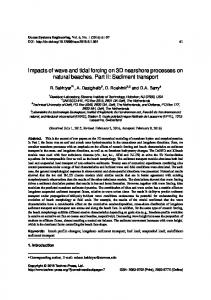
Survey frequency: Hours if necessary, typically days to months; spatial resolution: 1.5 m above ground. An easily accessible site facilitates regular visits of the instrument for maintenance and data retrieving, in the case data are stored in dataloggers. However, data can also be transmitted by radio, GSM, UMTS if the monitoring site is served by at least one of these technologies. A wise positioning of rain gauges should include at least one instrument close to the expected debris-flow triggering area.
9
Figure 2 A rainfall gauge installed upslope of a debris-flow initiation area
2.2 Flow characteristics Images and video recordings give an invaluable contribution to the recognition and interpretation of flow processes and effectively support quantitative monitoring performed by other sensors designed to record debris-flow depth and hydrographs. Amongst relevant debris-flow features that can be documented by video camera recordings, we mention the following: • variations in solid concentration and particle size, both between different debris flows and within the same event; • onset of turbulence corresponding to decrease in solid concentration (typically in the final phase of a debris-flow surge);
10
• presence and characteristics of precursory surges in the initial phase of a debris flow and secondary surges in the recession limb; • transport of large wood by the debris flow. In addition to the visual interpretation, video recordings provide the basis for automated or semi-automated recognition of important features of debris flows, such as grain size distribution (Genevois et al., 2001) or the presence of large boulders (Gomez and Lavigne, 2010). Moreover, several studies have demonstrated the suitability of video recordings (e.g. Arattano and Marchi, 2000; Genevois et al., 2001; Zhang and Chen, 2003) for recognizing debris-flow features in different parts of a channel reach. Surface velocity assessment from oblique video recordings could also be possible
applying
Large
Scale
Particle
Image
Velocimetry
(LSPIV)
algorithms. These methods are successfully used to measure velocities at the free surface of water streams (Muste et al., 2008). Zenithal recordings, achieved by video cameras installed vertically above the channel, shot a much smaller area, but permit easier assessment of flow characteristics, such as surface velocity distribution along the cross-section and particle size distribution of transported clasts. Cameras provided with image processing software are able to automatically evaluate the debris flow material movement (moving detection). This kind of software is able to recognize all the objects in function of their electromagnetic spectrum and to filter the data, in order to erase the noise elements such as the rainfall, allowing identifying only the moving debris flow material and thus potentially to issue a warning signal. To overcome the limitation of night view, videocameras can be installed with spotlights (Figure 3), which activation can be triggered by the exceeding of a certain threshold of data recorded by other sensors (e.g. raingauges, stage sensors). Alternatively, thermal cameras able to register the electromagnetic wave released by each material in function of its own
11
temperature could be used to record images at night, but the resolution of these devices is usually lower than that of normal videocameras.
Figure 3 A videocamera with spotlight (Gadria catchment, Italy)
2.3 Peak flow depth Without fixed instrumentations, the maximum debris flow depth can be measured during post-event surveys using theodolites or differential GPS thanks to the marks left on channel banks (Figure 4). Particular care must be taken to differentiate between the tracks left by the debris flow surface and the tracks left by the debris flow splashes (Aulitzky, 1989). A set of wires stretched at different levels across a cross-section can be also employed to monitor maximum depth of debris flows. These wires can detect the maximum depth according to the level of the highest wire that has been broken by the flow and also make it possible to record the time of occurrence of the surge at the instrumented site. However, after they have been broken, these devices cannot provide information about the height of further surges that follow the main one or about subsequent debris flows; they need to be reset each time after a debris flow. Photocells and infrared photobeam sensors can be utilized as a tool to detect debris flows (Chang,
12
2003). The flowing mass interrupts the beams emitted by the sensors, making it possible to detect the passage of the wave. If several sensors are installed at different heights at the same cross-section, it is also possible to approximately measure the peak flow stage.
Figure 4 An example of mud mark on a bank after the passage of a debris flow on the Réal Torrent in the French Alps; this kind of marks can be used to measure the flow depth during the peakflow discharge
2.4 Debris-flow hydrograph Debris flow depth represents the basis for the computation of other relevant variables such as flow velocity, discharge and volume. Different types of stage sensors can be used to monitor and record flow depth.
13
Ultrasonic sensors hung over the channel are the most used sensors to record debris-flow depths and hydrographs (Figure 5). These sensors are typically used to measure the hydrometric level in rivers and lakes. The strong and rapid variability of flow height with time in debris flows requires much shorter logging intervals between two consecutive recordings (1-2 seconds) than that used in water level measurements. Radar and laser sensors have also been used, similarly to ultrasonic sensors, to measure flow depth and record stage hydrographs of debris flows (Hürlimann et al, 2003; McArdell et al., 2007). Ultrasonic, radar and laser sensors work on a similar principle: the antenna of the sensor emits pulses that are reflected by the surface of the debris flow and received by the antenna as echoes. The running time of the pulses from emission to reception is proportional to the distance and hence to the level. The determined level is converted into an appropriate output signal and outputted as measured value. Badoux et al. (2009) outline about advantages and drawbacks of these three types of sensors: “Ultrasonic sensors are troublesome because under conditions of rapidly changing flow depth and splashing on the surface of the flow they sometimes do not return a signal (Hürlimann et al. 2003). Laser sensors provide high-quality data for debris flows (e.g., McArdell et al. 2007), but do not provide a useable signal for flood or hyper-concentrated flows. Radar sensors have a built in smoothing algorithm that provides a stable signal under conditions of rapidly changing flow depth or splashing on the surface of the flow, but the signal is delayed by a few seconds and changes in surface elevation are smoothed in comparison with laser sensors, making them somewhat less useful for research but reliable for warning”.
14
Figure 5 Example of ultrasonic and radar sensors deployed on a cable above a check-dam on the Réal Torrent in the French Alps
2.5 Ground vibration The passage of a debris-flow wave induces strong ground vibrations and underground sounds which can be recorded by different types of sensors (accelerometers,
velocimeters,
microphones;
Zhang,
1993;
Arattano,
1999; Suwa et al., 2011). The output signal of seismic sensors is a voltage proportional to the ground oscillation velocity that may be processed in different ways to extract more useful information, such as debris-flow hydrographs. An important advantage of ground vibration sensors is that they can be installed at a safe distance from the channel bed, overcoming an important limitation of other types of sensors which need to be hung over the channel and thus are more prone to damage. The vibration frequency associated with debris flows generally span the range from few Hz up to 300 Hz (Huang et al., 2007). It has to be noted that according to
15
the signal processing theory, the sampling rate at which the signal from the geophone has to be sampled to avoid aliasing must be at least twice the highest frequency of the signal itself. Furthermore, it is worthy to mention that attenuation of ground vibration in soil is extremely high; this issue requires
multiple
geophones
to
be
deployed
and/or
an
opportune
positioning. The attenuation, furthermore, is related to soil density, water content, matrix potential and porosity and generally scales inversely with respect to the frequency. Subsequently, the spectrum is usually dominated by lower frequency components. Nonetheless, due to the underlined requirements about sensitivity and sampling frequency, the electronics required to correctly sample the signal from the geophones and preserve data integrity present a significant challenge. The output signal of seismic sensors is currently processed with three different methods: the amplitude (Arattano, 1999), the impulses (Abancó et al., 2012), and the integration (Navratil et al., 2013a) methods. Seismic data processing with the amplitude method consist in transforming the signal from analogical to digital and then to calculate the mean absolute value every second (amplitude) to reduce the data amount. The amplitude (A) can be calculated as: n
A=
∑v i =1
i
n
(1)
where vi is the ground oscillation velocity, and n is the number of digital samples in each interval of recording. The data processing of debris-flow recordings obtained through ground vibration sensors returns graphs that strictly resemble the hydrographs recorded through ultrasonic, radar or laser sensors. A comparison between an hydrograph (black line) and an amplitude-versus-time-graph obtained with the previously described procedure (red line) for an event occurred in the Moscardo Torrent on June 22, 1996 is shown in Figure 6.
16
The impulses method is adopted in Switzerland and Spain (Abancó et al., 2012) monitoring sites to reduce the data amount and it consists in transforming the continuous signal (thick line in Figure 7) into a pulse signal (thin line in Figure 7) and then counting the number of impulses per each time interval. The impulses method requires the identification of a threshold value (red line in Figure 7) above which starting to count the impulses. If the chosen threshold is too low then the distinction between the phases of the event might become impossible. Another limitation of this method is the loss of information regarding the intensity of the signal. While the digitalization used by the amplitude method still conserves information
regarding
the
intensity,
namely
its
mean
value,
the
transformation into impulses loses this residual information. The integration method is implemented in France (Réal and Manival monitoring stations). An electronic signal processing unit is used to transform the output voltage of the geophone into an integrated signal that is sampled by the data logger unit (Campbell CR1000) at a frequency of 5 Hz. The signal processing unit is an electronic printed circuit specifically designed for the conditioning of analog signal from geophones. The unit first transforms the output voltage of the geophone into a rectified unidirectional signal (negative voltages are transformed into positive voltages). The rectified signal is then filtered with a 2.5 Hz cutoff frequency low-pass filter. The cutoff frequency was set at half the sampling frequency of the data logger to respect the Shannon criteria. This filtering is equivalent to applying a moving average on the raw signal, with a time period equal to 400 ms (Figure 8). The filtered signal is amplified and transformed into tension (mA) to be transported on long distances (up to 300 m). The main advantage of this method is that the geophone data can be sampled at a low frequency (5 Hz) while conserving the integral of the raw signal (total energy) from the geophone. It is nevertheless clear that
17
the frequency spectrum of the ground vibrations is lost, as well as the maximum range of ground vibration amplitudes. Soil properties of the river banks and location of each geophone determine specific offset and gain. Preliminary tests have been carried out with heavy boulders (approx. 10 kg) that were manually thrown into the torrent channel (3−4 m high) near geophones (Navratil et al., 2013a). Those tests showed that (1) the system can detect very low-magnitude ground vibrations, and (2) such recordings are consistent with nature and distance of triggering source from the geophone. By the same tests, it is also possible to calibrate the geophones. The magnitude of the signal mainly depends on the location of the geophone (on a bank, a boulder on a bank, and a check-dam, respectively), and, marginally, on the composition of the soil from the source to the geophone. Ultimately, it was found that the geophone fixed on big boulders embedded in a gravel deposit responds better. Remarkably, that data acquisition method has been successfully tested during several debris flows which occurred on the Réal Torrent since 2011 (Figure 9).
18
Figure 6 Comparison between an hydrograph (black line) and an amplitude-versus-timegraph (red line) for an event occurred in the Moscardo Torrent on June 22, 1996. The small differences between the hydrograph and the amplitude vs. time graph are due to the different locations of the sensors (geophones are installed around 1 km upstream ultrasonic sensors).
Figure 7 The transformation of the signal in the impulses method (from Abancó et al., 2012)
19
Figure 8 Numerical example of signal processing implemented in the integration method
Figure 9 Geophone recordings at Réal Torrent during the 29 June 2011 debris flow. (A) Upstream geophone Geo3A. (B) Middle stream geophone (Geo3B). (C) Downstream geophone (Geo3C). (D) The flow stage recorded by the ultrasonic sensor (US3_A at the same location as Geo3B); the reference elevation for US measurements (0 cm) corresponds to the channel bottom (From Navratil et al., 2013b)
Fiber optic sensors have also been proposed for monitoring ground vibrations caused by debris flows. The major advantage over conventional electronic-based sensors is the ability to separate the sensors from the electronics without any significant degradation in performance. This puts away the electronics from the hostile sensing environment. Furthermore, the performance matches or exceeds the performance of standard geophones and the sensor is intrinsically safe and immune to EMI/RFI. To our knowledge, there are very few examples in literature of employing fiber optic sensors for debris flow-induced ground vibration (Yin, 2012; Huang et al., 2012), but there are a large number of papers proposing
20
optical fiber geophones for similar application (e.g., oil & gas reservoir and micro-seismic exploration) so it is very likely this technology to break into this field and successfully compete with traditional geophones. Up to now, the large cost of deployment and maintaining represents the main drawback. 2.6 Mean flow velocity The characteristic steep debris-flow front can be detected and recognized in the
hydrographs
allowing
to
easily
perform
mean
front
velocity
measurements. By placing a pair of ultrasonic/radar/laser sensors or geophones at a known distance along a torrent, mean front velocity can be measured as the ratio between the distance between the sensors and the time interval elapsed between the arrival of the front at the two gauging sites (Figure 10). Mean velocity could also be computed from the records of other sensors using the same principle (e.g., wire detectors, photocells, microphones, etc.).
21
Figure 10 Flow depth measurement at two monitoring stations makes it possible to assess mean front velocity; (the horizontal scale is shortened with regard to both the distance between the sensors and the debris flow profile) (modified from Arattano and Marchi, 2008)
When ultrasonic/radar/laser sensors and seismic devices are used to measure mean front velocity, debris-flow front and/or other specific recognizable features must be present in their graphs. However such features may not be always present in the graph. The use of cross correlation techniques, that are commonly used in signal processing, may allow the use of graphs that do not show a clear front or other evident recurrent features, to estimate at least the mean velocity of the entire wave. In general, cross-correlation can be defined as the correlation of a series with another series, shifted by a particular number of observations and its function can be expressed as follow:
φ xy (τ ) =
+∞
∑x y
t = −∞
t
t +τ
(2)
where xt is the function that expresses the recorded signal at the upstream sensor at the time t and yt+τ is the function that gives the recorded signal at the downstream sensor at the time t+τ. The maximum value of the function φxy allows an estimation of the value of τ., that is the time needed by the debris flow to propagate between the two sensors, and allows to determine the mean velocity of the wave (Figure 11). If the distance between the two locations is known, the velocity can then be easily assessed. Therefore, given a certain phenomenon that produced a recorded at two different locations, the cross correlation analysis allows to determine, with an objective method, the time interval elapsed between the appearance of that phenomenon at the first and at the second location.
22
The cross correlation technique may allow a comparison between the mean front velocity, when a front is present, and the mean velocity of the entire wave, which may be significantly different sometimes. As far as the estimation of the volume of the debris flow using two hydrographs is concerned, the use of the velocity of the entire wave would be preferable to get a more consistent estimation when it differs from the mean front velocity.
Figure 11 Cross correlation applied to debris-flow amplitude data from geophones records.
2.7 Peak discharge and volume The measurement of debris-flow depth and the assessment of mean flow velocity provide the elements for estimating discharge and total debris flow volume. The flow area occupied at different times along a debris-flow wave is obtained from stage measurements and topographic surveys of the
23
cross-section geometry. Discharge can be computed as the product of the mean flow velocity by the cross-sectional flow area. Total discharged volume is then computed by integrating debris flow discharge on the hydrograph: tf
Vol = U ∫ A(t )dt t0
(3)
where A(t) is the cross section area occupied by the flow at the time t, U is the mean flow velocity, t0 is the time of arrival of the surge at the gauging site and tf - t0 is the overall time interval of the debris flow. This approach can be applied only in cross-sections in which the debris flow did not cause significant topographic changes. The approach to computing the flowing volume presented in eq. 3 assumes that the material flows through the considered section at a constant velocity during the surge. Usually the value of U is assumed as the value of the mean velocity of the front. However measurements, carried out using video pictures, have shown that an increase of velocity may occur behind the front and then surface velocity remains higher than front velocity for a significant portion of the debrisflow wave (Marchi et al., 2002). Using mean front velocity in eq. 3 could then result in an underestimation of debris-flow volumes. Since mean velocity may vary remarkably during the surge, debris-flow volumes assessed using eq. 3 should be considered as approximate estimates. If flow velocity measurements are available for various phases of the event, they can be used to refine the volume assessment. Since mean front velocity and the mean velocity of the entire wave, obtained through cross-correlation, may significantly differ sometimes, as mentioned previously, the use of the latter would be preferable to get a more consistent estimation when this difference is significant.
24
2.8 Overview of additional devices In addition to the devices and methods employed for monitoring debrisflow
main
parameters
described
in
the
previous
sections,
several
additional parameters can be also measured to collect more information on debris flows (Table 2). Infrasound monitoring system can be used for debris-flow monitoring purposes (Zhang et al., 2004; Chou et al., 2007; Kogelnig et al., 2011). Infrasound signals generated by mass movement have a specific amplitude and occupy a relatively noise-free band in the low-frequency acoustic spectrum. The low-frequency fluctuations in the air can be detected by an infrasound microphone (Kogelnig et al., 2011). The main advantages of this method are similar to those of geophones (e.g., monitoring with a safe distance from the channel bed) whereas problems are mainly given by noise induced from other sources (e.g., human activity, wind). Doppler speedometers, which operating principle is based on measuring the frequency of radio waves reflected by a moving object, can be applied to measure surface velocity of a debris flows. In the case of debris flows the target for the measurement can be the front of a debris flow, a surface wave, a coarse particle or a piece of woody debris moving on the surface (Arattano and Marchi, 2008). Several other methods exist to measure surface velocity: spatial filter velocimetry (Itakura and Suwa, 1989), spatio-temporal derivative space method (Inaba et al., 1997), image processing techniques (see section 2.2). The load of the debris-flow mass can be measured by installing load cells at the channel bottom (Genevois et al., 2000). If vertical and horizontal load cells are mounted on a force plate normal and shear stresses can also be measured (McArdell et al., 2007). As demonstrated in the Illgraben (McArdell et al., 2007), measuring normal stress in combination with the flow depth, is essential for the assessment of the mean bulk density of the flowing debris and its variation with time. Another parameter of the flowing debris, the pore fluid pressure, can be measured by installing pressure
25
transducers at the bottom of the channel (Berti and Simoni, 2005; McArdell et al., 2007). An important debris-flow parameter that deserve to be measured for improving the design of debris-flow control works is the impact force. The impact force exerted by debris flows
on obstacles along the path (e.g.
buildings, check dams, defensive walls) can be measured by using pressure mark gauges installed on dam walls or large boulders (Okuda et al., 1980) or strain sensors (Zhang, 1993; Hu et al., 2011b), which allow continuous measurements. Berger et al. (2011) constructed erosion sensor columns to monitor erosion depth and timing. A sensor column of a given length is composed of several cylindrical aluminum tubes, each of them containing an electronic resistor connected to the resistor of the overlying and underlying elements. When channel-bed erosion induced by a debris flow breaks the connection between one or more elements, a drop in total resistance occurs. This drop in total resistance, recorded on a data logger, can be related to the change in the length of the sensor column to determine the timing and the depth of erosion. Finally, topographic surveys of debris-flow deposits (Figure 12) and variations in sediment sources and channel storage (Figure 13) deserve to be mentioned here as they permit comparison with debris-flow volumes assessed
from
debris-flow
hydrographs
(section
2.7).
Topographic
measurements and detection of geomorphic changes caused by debris flows can obviously be performed also in catchments not instrumented for the monitoring of debris-flow waves. They could thus be viewed as an approach
to
debris-flow
monitoring
complementary
to
systematic
observations in catchments equipped with permanent devices: although limited
to
post-event
volume
assessment
and
geomorphic
change
detection, topography-oriented monitoring enables observations in a potentially large number of sites.
26
Figure 12 Map of sediment thickness deposited in the retention basin in the Gadria catchment (Italy) during a debris flow, evaluated as the difference between two TLSderived DTMs
27
Figure 13 Topographic changes after debris-flow and bedload-transport events on a reach of the Manival Torrent from terrestrial laser scanning resurveys (Theule, 2012)
28
3
Suitability of debris-flow monitoring methods
In Table 3 are listed the suggested acquisition parameters for the main devices commonly applied for debris flow monitoring. Table 4 presents a classification in terms of suitability of debris-flow monitoring devices concerning specific parameters. Table 3 Suggested acquisition parameters for different instruments used in debris flow monitoring Instrument type
Variable to monitor
Recording
Other parameters/note
intervals Raingauge
Rainfall
1-5 min
0.2 mm bucket
1-2 s
Radar
intensity/depth Stage sensor
Flow depth
sensors
seem
more
reliable Geophone
Ground velocity
1-2 s
Natural
frequency
of
the
sensor around 10 Hz Amplification
factor:
depending on the geology of the site and distance of the source Videocamera
Flow images
8-10 fps
Image resolution depends on videcamera-flow distance and on the purpose (LSPIV vs simple flow description)
Load cell
Flow
pressure
and
1-2 s
shear stress Laser-doppler
Surface velocity
1-2 s
Pore-fluid pressure
1-2 s
speedometer Piezometer
phone
Micro-
ometers
speed-
Doppler
partially suited for measuring this parameter
camera
Video-
suited for measuring this parameter
sensor
Pendulum
Surface velocity
sensor
Fiber optic Wire
highly suited for measuring this parameter
discharge and volume
phone
Geo-
Mean flow velocity, peak
Debris flow “hydrograph”
Ground vibration
Peak flow depth
sensor
sensor
sensor
Laser
Ultrasonic Radar
Debris-flow occurrence
Parameters of interest
29
not suited for measuring this parameter
Table 4 Suitability of debris-flow monitoring devices concerning specific parameters
30
4 References Abancó
C.
Hürlimann
M.,
Fritschi
B.,Graf
C.
Moya
J.
(2012)
-
Transformation of Ground Vibration Signal for Debris-Flow Monitoring and Detection in Alarm Systems. Sensors,12, 4870-4891. Arattano M. (1999) - On the use of seismic detectors as monitoring and warning systems for debris flows. Natural Hazards, 20(2-3): 197-213. Arattano M., Deganutti A.M., Marchi L. (1997) - Debris flow monitoring activities in an instrumented watershed on the Italian Alps. Debris-Flow Hazards Mitigation: Mechanics, Prediction & Assessment: 506-515. Arattano M., Marchi L. (2000) - Video-derived velocity distribution along a debris flow surge. Physics and Chemistry of the Earth part B, 25 (9): 781784. Arattano M., Marchi L. (2005) - Measurements of debris flow velocity through cross-correlation of instrumentation data. Natural Hazards and Earth System Sciences, 5(1): 137-142. Arattano M., Marchi L. (2008) - Systems and sensors for debris-flow monitoring and warning. Sensors, 8(4): 2436-2452. Aulitzky, H. (1989). The debris flows of Austria. Bulletin of the International Association of Engineering Geology, 40: 5-13. Bacchini, M., Zannoni, A. (2003) - Relations between rainfall and triggering of debris-flow: case study of Cancia (Dolomites, Northeastern Italy). Natural Hazards and Earth System Science, 3(1-2): 71-79. Badoux A., Graf C., Rhyner J., Kuntner R., McArdell B.W. (2009) - A debrisflow alarm system for the Alpine Illgraben catchment: design and performance. Natural Hazards, 49(3): 517-539. Berger C., McArdell B.W., Schlunegger F. (2011) - Direct measurement of channel erosion by debris flows, Illgraben, Switzerland. Journal of Geophysical Research-Earth Surface, 116.
31
Berti M., Simoni A. (2005) - Experimental evidences and numerical modelling of debris flow initiated by channel runoff. Landslides, 2, 171-182. Caine N. (1980) - The rainfall intensity–duration control of shallow landslides and debris flows. Geografiska Annaler, A, 62: 23–27. Chang S.Y. (2003) - Evaluation of a system for detecting debris flows and warning road traffic at bridges susceptible to debris-flow hazard. DebrisFlow Hazards Mitigation: Mechanics, Prediction, and Assessment, Vols 1 and 2: 731-742. Chou H.T., Cheung Y.L., Zhang S. (2007) - Calibration of infrasound monitoring system and acoustic characteristics of debris-flow movement by field studies. Debris-Flow Hazards Mitigation: Mechanics, Prediction, and Assessment, 571–580. Coe J.A., Kinner D.A., Godt J.W. (2008) - Initiation conditions for debris flows generated by runoff at Chalk Cliffs, central Colorado. Geomorphology, 96(3-4): 270-297. Genevois R., Galgaro A., Tecca P.R. (2001) - Image analysis for debris flow properties estimation. Phys. Chem. Earth (C), 26, 9, 623-631. Genevois R., Tecca P.R., Berti M., Simoni A. (2000) – Debris flow in the Dolomites: Experimental data from a monitoring system. Proceedings of the Second International Conference on Debris-flow Hazards Mitigation: Mechanics, Prediction, and Assessment, Taipei, Wieczorek, G.; Naeser, N.; Eds.; A.A. Balkema, Rotterdam, 283-291. Gomez C., Lavigne F. (2010) - Automated block detection in lahars through 3-bands spectral analysis of video images. Journal of Volcanology and Geothermal Research, 190, 379–384. Guzzetti F., Peruccacci S., Rossi M., Stark C.P. (2008) - The rainfall intensity-duration control of shallow landslides and debris flows: an update. Landslides, 5(1): 3-17.
32
Hu K., Hu C., Li Y., Cui P. (2011a) - Characteristics and mechanism of debris-flow surges at Jiangjia Ravine. In: Genevois R., Hamilton D.L., and Prestininzi A. (eds), 5th International Conference on Debris-Flow Hazards Mitigation: Mechanics, Prediction and Assessment, Casa Editrice Università La Sapienza, Roma, pp 211-217. Hu K., Wei F., Li Y. (2011b) Real‐time measurement and preliminary analysis of debris‐flow impact force at Jiangjia Ravine, China. Earth Surf. Process. Landforms 36, 1268–1278, DOI: 10.1002/esp.2155 Huang C.J., Yin H.Y., Chen C.Y., Yeh C.H., Wang C.L. (2007). Ground vibrations produced by rock motions and debris flows. Journal of Geophysical Research, 112, F02014, doi:10.1029/2005JF000437. Huang C.-J., Chu, C.-R., Tien, T.-M., Yin H.-Y., Chen, P.-S. (2012) Calibration and deployment of a Fiber-Optic Sensing system for monitoring debris flows. Sensors, 12 (5): 5835-5849. Hungr O., Morgan G.C., Van Dine D.F., Lister R.D. (1987) - Debris flow defenses in British Columbia. In:
Costa J.E. and Wieczorek G.F. (eds),
Debris Flows / Avalanches: Process, Recognition, and Mitigation, Geological Society of America, Reviews in Engineering Geology, 7: 201-222. Hürlimann M., Abancó C., Moya J., Raïmat C., Luis-Fonseca R. (2011) Debris-flow monitoring stations in the Eastern Pyrenees. Description of instrumentation, first experiences and preliminary results. In: Genevois R., Hamilton D.L., and Prestininzi A. (eds), 5th International Conference on Debris-Flow Hazards Mitigation: Mechanics, Prediction and Assessment, Casa Editrice Università La Sapienza, Roma, pp 553–562. Hürlimann M., Rickenmann D., Graf C. (2003) - Field and monitoring data of debris-flow events in the Swiss Alps. Canadian Geotechnical Journal, 40(1): 161-175. Inaba H., Uddin M.S., Itakura Y., Kasahara M., 1997. Surface velocity vector field measurement of debris flow based on spatio-temporal derivative space method. Proceedings of the First International Conference
33
on Debris-flow Hazards Mitigation: Mechanics, Prediction, and Assessment, 757-766. Itakura Y., Inaba, H., Sawada, T, 2005. A debris-flow monitoring devices and methods bibliography. Natural Hazards and Earth Systems Sciences, 5, 971-977. Itakura, Y., Suwa, H., 1989. Measurement of surface velocity of debris flows by spatial filtering velocimetry. Proceedings of the Japan-China Symposium on Landslides and Debris Flows, Tokyo, 199-203. Kogelnig A., Hübl J., Suriñach E., Vilajosana I., McArdell B. (2011) Infrasound produced by debris flow: propagation and frequency content evolution. Natural Hazards, DOI 10.1007/s11069-011-9741-8. Marchi L., Arattano M., Deganutti A.M. (2002) - Ten years of debris-flow monitoring in the Moscardo Torrent (Italian Alps). Geomorphology, 46(12): 1-17. McArdell B.W., Bartelt P., Kowalski J. (2007) - Field observations of basal forces and fluid pore pressure in a debris flow. Geophysical Research Letters, 34(7). McCoy S.W., Coe J.A., Kean J.W., Staley D.M., Wasklewicz T.A., Tucker G.E. (2011) - Observations of debris flows at Chalk Cliffs, Colorado, USA: part 1, in-situ measurements of flow dynamics, tracer particle movement and video imagery from the summer of 2009. In: Genevois R., Hamilton D.L., and Prestininzi A. (eds), 5th International Conference on Debris-Flow Hazards Mitigation: Mechanics, Prediction and Assessment, Casa Editrice Università La Sapienza, Roma, pp 715–724. Muste M., Fujita I., Hauet A., 2008. Large-scale particle image velocimetry for measurements in riverine environments. Water Resources Research, 44, Doi 10.1029/2008wr006950. Navratil O., Liébault F., Bellot H., Theule J., Travaglini E., Ravanat X., Ousset F., Laigle D., Segel V., Fiquet M., (2012) - High-frequency
34
monitoring of debris flows in the French Alps. Proc. 12th Interpraevent congress, Grenoble, 281-291. Navratil O., Liébault F., Bellot H., Theule J., Ravanat X., Ousset F., Laigle D., Segel V., Fiquet, M., (2013a). Installation d'un suivi en continu des crues et laves torrentielles dans les Alpes françaises. Mémoires de la Société Vaudoise des Sciences Naturelles, 25: 83-97. Navratil O., Liébault F., Bellot H., Travaglini E., Theule J.I., Chambon G., Laigle D., (2013b). High-frequency monitoring of debris-flow propagation along the Réal Torrent, Southern French Prealps. Geomorphology. DOI: 10.1016/j.geomorph.2013.06.017 Okuda S., Suwa H., Okunishi K., Yokoyama
K., Nakano M. (1980) -
Observations on the motion of a debris flow and its geomorphological effects. Zeitschrift für Geomorphologie., Suppl. Bd., 35: 142–163. Pierson T. C. (1986) - Flow behavior of channelized debris flows, Mount St. Helens, Washington. In: Abrahms A. D. (ed), Hillslope Processes, Allen & Unwin, Boston, 269–296. Suwa H., Okano K., Kanno
T. (2011) - Forty years of debris flow
monitoring at Kamikamihorizawa Creek, Mount Yakedake, Japan. In: Genevois R., Hamilton D.L., and Prestininzi
A. (eds), 5th International
Conference on Debris-Flow Hazards Mitigation: Mechanics, Prediction and Assessment, Casa Editrice Università La Sapienza, Roma, pp 605–613. Tecca P.R., Galgaro A., Genevois R., Deganutti A.M. (2003) - Development of a remotely controlled debris flow monitoring system in the Dolomites (Acquabona, Italy). Hydrological Processes, 17(9): 1771-1784. Theule J.I., 2012. Geomorphic study of sediment dynamics in active debrisflow catchments (French Alps), Unpublished PhD thesis, Université de Grenoble, Grenoble, 152 pp. Wilson R. C., Mark R. K., Barbato G. (1993) - Operation of a Real-time warning system for debris flows in the S. Francisco Bay Area, California. In:
35
Hsieh Wen Shen, S. T. Su e Feng Wen (eds), Hydraulic Engineering '93 vol. 2,
ASCE
1993
National
Conference
on
Hydraulic
Engineering
and
International Symposium on Engineering Hydrology, American Society of Civil Engineers, New York, pp 1592-1597. Yin
H.-Y.
(2012)
Debris-flow
monitoring
and
warning
in
Taiwan.
International workshop “Monitoring bedload and debris flows in mountain basins”, Bolzano – Bozen (Italy), October 10-12, 2012 Yin H.-Y., Huang C. J., Chen C. Y., Fang Y. M., Lee, B. J., Chou, T. Y. (2011) - The present development of debris flow monitoring technology in Taiwan – A case study presentation. In: Genevois R., Hamilton D.L., and Prestininzi A. (eds), 5th International Conference on Debris-Flow Hazards Mitigation: Mechanics, Prediction and Assessment, Casa Editrice Università La Sapienza, Roma, pp 623–631. Zhang S. (1993) - A Comprehensive Approach to the Observation and Prevention of Debris Flows in China. Natural Hazards, 7(1): 1-23. Zhang
S.,
Chen
J.
(2003)
-
Measurement
of
debris-flow
surface
characteristics through close-range photogrammetry. In: Rickenmann D, Chen C-L (eds) Debris-flow hazards mitigation: mechanics, prediction, and assessment. Proceedings of the third international conference. Millpress, Rotterdam: 775–784. Zhang S., Hong Y., Yu B. (2004) - Detecting infrasound emission of debris flow for warning purposes. Internationales Symposium Interpraevent VII: 359–364
Part III Protocol for Wood Monitoring
WP5 - Action 5.2 Protocols on standardized data collection methods in sediment transport monitoring for transboundary exchange Lead authors: Hervé Piegay (PP8) Contributors: Mario Aristide Lenzi, Lorenzo Picco & Diego Ravazzolo (all PP03)
June, 2013
1
Contents
Introduction
2
1
5
Wood tracking devices and methods
1.1
Wood tracking using RFID
7
1.2
GPS Track
9
2
Wood passage censing using video monitoring
10
2.1
Semi-manual detection of wood
12
2.2
Wood volume calculation
13
2.3
Actual limitations and error estimate
16
2.4
Perspectives in automatic detection of wood
17
3
Suitability of wood monitoring methods
References
24 25
2
Introduction Large wood is an important component of river systems, because it contributes to many different processes as geomorphic, hydraulic, and ecological (Brookes, 1988; Gurnell et al., 2002; Sedell et al., 1988). On the other side, wood in-channel transported during flood events could be a problem for some human activities on rivers as, for example, commercial marine operations on large rivers (Gurnell et al., 2002; Piégay, 2003). It represents a risk for flooding and human infrastructure (Bradley et al. 2005, Comiti et al. 2006), notably when it accumulates on or near to sensible structures as bridge piers (Wallerstein, 1998; Kothyari and Ranga Raju, 2001). Wood in rivers can be an obstacle for flows during floods, exacerbating locally flooding and infrastructure damages. There is a need for data to calibrate wood budgets and examine processes related to the transport of wood during floods (Benda and Sias 2003, Hassan et al. 2005).
Previous studies of wood in rivers have quantified
spatial distributions but temporal dynamics remain poorly documented. The lack of such data is related to limitations inherent in existing methods, especially when applied to large rivers. For these reasons, and also for a better management of the river system, it is important to understand where the wood is recruited, moves and where it tends to accumulate system (Curran, 2010). However, the dynamic and mobility of large wood in rivers is poorly understood, especially in wide gravel-bed rivers. There is still a considerable lack of knowledge on the complex set of processes involved in the recruitment, transport and deposition of woody elements all over the fluvial systems. Even more on the quantification of these processes at the range of spatial and temporal scales at which they occurred. Only a few studies focused on this kind of surveys, requiring a lot of time (Table 1).
3
Large wood (LW) can be defined as the woody elements (including roots and branches) characterized by 1 m or more of length and diameter greater than 0.1 m or both (Jackson and Sturm, 2002). Five existing technologies were field-tested by MacVicar et al. (2008) to assess their utility for quantifying the temporal dynamics in rivers: passive Radio
Frequency
transponders,
Identification
radio
transmitters,
(RFID) video
transponders, monitoring,
Active
RFID
repeated
high-
resolution aerial photos (produced by a low-flying drone aircraft). Passive RFID transponders and radio transmitters are reliable for wood tracking. Radio transmitters are suited to multi-year (~ 5 year) surveys and can be detected at 800 m, whereas passive RFID transponders are limited by a read range of 0.30 m but suited for longer term studies. Active RFID transponders combine a moderate read range (With an antenna) and low cost with the ability to monitor wood transport during floods but require more testing.
Video monitoring is used to monitor the wood passage
within a given section.
Amongst these 5 technologies, 2 are detailed here (RFID tracking and video) and a new one is available based on GPS tracking.
4
Table 1 Summary of previous field studies of wood movement and wood deposit renewal in river Survey Reference
Techniques
Type of survey
River
Drainage 2
Area (km )
distance (km)
Lienkaemper and
Field survey –
Key pieces,
Swanson (1987)
visual
unlogged
Field survey – Bilby (1984)
numbered
Post logging
tags Field survey – Keim et al. (2000)
numbered tags Field survey –
Haga et al. (2002)
numbered tags
Jacobson et al. (1999)
Andreoli et al (2007)
Piégay and Marston (1998)
logging
and Hudson
Reco-
n
very (%)
tion (yr)
6.0
0.11
1 flood
42
9.0
1.10
0.5
74
3
21
100a
~80 in first flood
7.0 – 15.6
0.45 – 0.70
76
Creeks Uniform 1.6 m long pieces
ephemeral
tags
stream
Field survey
dura-
Bark,
In-situ wood,
tags
Creek
Buttermilk,
numbered
numbered
Salmon
key pieces post
Field survey -
Field survey –
Mack Creek
Study
Oyabu Creek
5.3
5.5
1
63
Kuiseb River
14,700
160
1 flood
2105
9 - 13
1.5 – 1.8
1
3,630
point
3
95 in first flood
21
2 mountain All wood > 0.1
basins of
m diameter
Southerns
322 -
98 - 100
381
Andes Channel bank
Ain River
1 jam
-
random Van der Nat et al. (2003)
Field survey
In-channel wood
Tagliamento River
2,580
4
2
locations in 2
-
reaches Haschenburger and Rice (2004) Lassettre et al. (2007)
Aerial
Aerial
Jams only Helicopter photograph
Moulin and Piégay
Point survey -
All transported
(2004)
reservoir
wood
Point survey -
All transported
reservoir
wood
Seo et al. (2008)
Notes
Carnation
11
3
7
Ain River
3,760
40
10
Rhône River
10,910
point
10
6.2 – 2,370
point
1–29
Creek
131 reservoirs in
5 jams 445 –
-
-
1008 13,000 m3/yrb
100
300 –
Japan
a) Transported wood was stopped in downstream reservoir b) Volume of wood trapped in reservoir. c) Volume of wood trapped in reservoir converted into mass of carbon.
400,000 kgC/yr
c
100
5
1 Wood tracking devices and methods This protocol focuses on the devices used for monitoring the mobility and displacement of LW during and after flood events. We also present the methods commonly employed to measure the most relevant parameters for LW investigations. It is known that in wide rivers, there are some problems to survey the LW along the entire active channel area. This is the reason because it is necessary to adopt a sampling procedure identifying cross-sectional transects which limit the reliability of LW storage (Gurnell et al., 2000a; 2000b). Field surveys can be carried out using the guideline of a spread sheet to measure different characteristics such as, for example, the state of decay, orientation to flow and position in the channel (Table 2). Volume of LW is identified through its mid-diameter and length measured using tree caliper and tape, respectively (Mao et al., 2008).
Log mobility and
displacement during and after flood events can be measured applying two monitoring techniques: implanting radio frequency identification (RFID) tags in logs (McVicar et al., 2009) and using GPS Track devices.
6
Table 2 Example of spread sheet guidelines for LW survey
7
1.1 Wood tracking using RFID
Passive
Radio
Frequency
Identification
(RFID)
transponders,
originally
developed for security and commercial purposes, also known as Passive Integrated Transponder (PIT) tags, have previously been applied to track the movements of fish (Feldheim et al., 2002) and sediment particles (Lamarre et al., 2005) in rivers. RFID technology uses electromagnetic coupling to transmit an identification code as ‘noise’ on a radio frequency signal. This code is unique to each tag, while the transmission frequency is shared.
Passive RFID
transponders are transponders, which means that they transmit a signal in response to an incoming signal.
The energy used to transmit the signal is
taken from the received signal, and the tags do not have batteries.
While a
range of transponder shapes and sizes are commercially-available, this study used a hermetically sealed 23 x 4 mm glass cylinder transponder (Figure 1) transmitting at (134.2 kHz) that was developed by TIRIS Technology. The tags are detected using a portable control unit and antenna.
Key advantages of
these tags are that they can be programmed with unique identification codes, which allows a precise spatial analysis of wood mobilisation and deposition; the durability of the tags in extreme environments; and the lack of a battery, which allows long term studies. An important limitation of the technique is that the detection range is only about 30 cm for the tag and antenna combination that was used in this study.
Figure 1 Example of passive RFID tag of TIRIS Technology composed by 23.4 mm glass cylinder transponder transmitting at (134•2 kHz).
8
Active RFID transponders are similar to passive RFID transponders in that they use electromagnetic coupling on a shared radio frequency to allow the remote identification of unique tags. Active RFID transponders are transmitters, however, and they emit a beacon signal at a predetermined time interval. While a range of tags are available from different companies, this study utilized 433 MHz tags purchased from RFCode Inc. Each tag is enclosed in a shock and splash-resistant polycarbonate case that is 47 x 34 x 12 mm in size (Figure 2). They use a replaceable coin cell battery. Fixed and mobile readers are available so that the techniques allowed to survey wood deposit and mobilisation as well as wood input from floodplain but also censing the wood output from the study reach (Q0) which is was not possible with the previous tracking techniques so that it is not possible to know if wood piece disappeared because the signal is not captured or because they moved away. The mobile reader can be clipped onto a belt and communicates via Bluetooth™ to a handheld computer.
A
significant advantage of this technique is that the detection range with the fixed reader (~300m) is sufficient to detect tags from a streamside station in many rivers.
The principal disadvantage is that the signal transmission requires
batteries, which limits the lifetime of the tag. These tags have not previously been tested in rivers.
Figure 2 Example of active RFID tag are those of the company RFCode Inc in which each tag is enclosed in shock resistant and splash resistant case that is 47-34-12 mm in size.
9
Both mobile and fixed readers are available. We installed the software supplied with the mobile reader by RFCode on a Trimble GeoXT Handheld GPS. A fixed reader was installed at a gauging station. A Tavis data router was connected to the reader and equipped with a memory card to record the identification codes of detected trees and their time of passage. Two Yagi antennae were installed on a pole outside of the station pointed across and upstream on the river. The gauging station is equipped with electrical and telephone connections. 1.2
GPS Track
This technique of LW monitoring has never been tested before in rivers monitoring activities, consents to record the displacement of a log during a flood event using a GPS track devices (passive or active). The aspect that distinguishes the active from a passive GPS track is the capacity to send, in real time, Short Message Service (SMS) over GSM communications network (i.e. time, position, batteries lifetime). An example of active GPS track device is the Trim Trac Locator by Trimble (Figure 3). This GPS track has dimensions of 143 mm x 76 mm x 38 mm and weight of 205 grams (not including batteries). The device work with 4 AA batteries which permit to operate up to 90 days under typical usage with good GPS signal strength. The device is composed by an internal GPS antenna and it has a cold start GPS acquisition time, warm start and hot start GPS of