Provably Fast Training Algorithms for Support Vector ... - CiteSeerX

Provably Fast Training Algorithms for Support Vector Machines
Jos´e L. Balc´azar Departament de Llenguatges i Sistemes Inform`atics, Univ. Polit`ecnica de Catalunya Campus Nord, Jordi Girona Salgado 1-3, 08034 Barcelona, Spain Yang Dai Dept. of Bioengineering (MC063) University of Illinois at Chicago 851 S. Morgan Street, Chicago, IL 60607–7052, USA Osamu Watanabe Dept. of Mathematical and Computing Sciences, Tokyo Institute of Technology Meguro-ku Ookayama, Tokyo 152-8552, Japan

Abstract Support Vector Machines are a family of data analysis algorithms, based on convex Quadratic Programming. We focus on their use for classification: in that case the SVM algorithms work by maximizing the margin of a classifying hyperplane in a feature space. The feature space is handled by means of kernels if the problems are formulated in dual form. Random Sampling techniques, successfully used for similar problems are studied here. The main contribution is a randomized algorithm for training SVMs for which we can formally prove an upper bound on the expected running time that is quasilinear on the number of data points. To our knowledge, this is the first algorithm for training SVMs in dual formulation and with kernels for which such a quasilinear time bound has been formally proved.
The first author started this research while visiting the Centre de Recerca Matem`atica of the Institute of Catalan Studies in Barcelona, and is supported by the IST Programme of the EU under contract number IST1999-14186 (ALCOM-FT), EU EP27150 (Neurocolt II), Spanish Government PB98-0937-C04 (FRESCO), and CIRIT 1997SGR-00366. The second author conducted this research while at the Dept. of Mathematical and Computing Sciences, Tokyo Institute of Technology, and is supported by a Grant-in-Aid (C-13650444) from the Ministry of Education, Science, Sports and Culture of Japan, and a start-up fund from Dept. of Bioengineering, University of Illinois at Chicago. The third author started this research while visiting the Centre de Recerca Matem`atica of the Institute of Catalan Studies in Barcelona, and is supported by a Grant-in-Aid for Scientific Research on Priority Areas “Discovery Science” from the Ministry of Education, Science, Sports and Culture of Japan. We want to thank for their help Emo Welzl, Nello Cristianini, and John Shawe-Taylor.

1. Introduction The Support Vector Machine (SVM in short) is a modern mechanism for two-class classification, regression, and clustering problems. Since the present form of SVM was proposed [CV95], SVMs have been used in various application areas, and their classification power has been investigated in depth from both experimental and theoretical points of view [CST00]. An important feature is that their way of working, by identifying the so-called support vectors among the data, offers important contributions to a number of problems related to Data Mining. Indeed, the outcome of the training phase of a SVM is a set of weights associated to the input data; the weight is null on all data except the support vectors. In most situations only a small fraction of the data become support vectors, and it can be rigorously proven that the same outcome of the training is obtained if one only uses support vectors instead of all the data points. Therefore SVMs can be used for data summarization. It has been experimentally shown [SBV95] that, for some relevant tasks, the set of support vectors is stable in the sense that several different SVM-based classifiers ended up all choosing large ratios of common support vectors; thus, indeed this suggests that the support vectors are capturing the essentials of the data set. Finally, in a phase of data cleaning, outliers are easily detected by monitoring the growth of the weights. A more detailed, accessible survey of the method and references to applications to data mining and many other tasks is [BC00]. The three main characteristics of SVMs are: first, that

they minimize a formally proven upper bound on the generalization error; second, that they work on high-dimensional feature spaces by means of a dual formulation in terms of kernels; and, third, that the prediction is based on hyperplanes in these feature spaces, which may correspond to quite involved classification criteria on the input data, and which may handle misclassifications in the training set by means of soft margins. The bound on the generalization error, to be minimized through the training process, is related to a data-dependent quantity (the margin, which must be maximized) but is independent of the dimensionality of the space: thus, the socalled “curse of dimensionality”, with its associated risk of overfitting the data, is under control, even for infinitedimensional feature spaces. The handling of objects in high-dimensional feature space is made possible (and reasonably efficient) through the use of the important notion of “kernel” [BGV92]. If the maximization of the margin is expressed in dual form, it turns out that the only operations needed on data, both to train the SVM and to classify further data, are scalar products. A kernel is a function that operates on the input data but has the effect of computing the scalar product of their images in the feature space: this allows one to work implicitly with hyperplanes in highly complex spaces. We will come back to duality in section 5, and we defer the detailed explanation of the last feature, the soft margins approach, to the next section. Algorithmically, the problem amounts to solving a convex quadratic programming (QP in short) problem; actually, it was proved in [SBV95] that a similar technique is able to help choosing a kernel. However, to scale up to really large data sets, the standard QP algorithms alone are inappropriate since their running times grow too fast [BC00]. Thus, many algorithms and implementation techniques have been developed for training SVMs efficiently. Among the proposed speed-up techniques, those called “subset selection” have been used as effective heuristics already from the earliest papers eventually leading to SVM, including [BGV92]. Roughly speaking, a subset selection is a technique to speed-up SVM training by dividing the original QP problem into small pieces, thereby reducing the size of each QP problem. Well-known subset selection techniques [CST00] are chunking, decomposition, and sequential minimal optimization [Pla99] (SMO in short), which may be combined with a reduction on the data on the basis of socalled guard vectors [YA00]. In particular, SMO has become popular because it outperforms the others in several experiments. Though the performance of these subset selection techniques has been extensively examined, no theoretical guarantee has been given on the efficiency of algorithms based on these techniques. As far as the authors know, the only positive theoretical results are the convergence (i.e.,

termination) of some of such algorithms [Lin01, KG01]. Yet another recent alternative, the Reduced Support Vector Machine [LM01], proposes to use only a single random subsample of data points, and to combine it to all the data points through kernel-computed scalar products in feature space. Our approach has some resemblance with this one in that a random selection of a small number of data points is made; however, in our algorithms, this is done repeatedly by filtering the selection through a probability distribution that evolves according to the results of the previous phases. We focus on algorithms for training two-class classification SVMs. In a previous paper [BDW01], we have proposed to use random sampling techniques that have been developed and used for combinatorial optimization problems. An important drawback of our previous algorithm in [BDW01], or, rather, of its analysis, based on the beautiful Simple Sampling Lemma of [GW00], is that the algorithm is analyzed in primal form, and that the analysis of its running time is not valid, in principle, for its natural dual counterpart. The reason is that the linearly many new variables that appear as Lagrange multipliers in the dual formulation increase the dimensionality too much. Additionally, the analysis depended on certain unproven combinatorial hypothesis. The contribution of this paper is a randomized subset selection scheme that improves on our previous algorithm in that it can be applied in dual form, and in that the theorem that bounds the expected number of rounds does not depend on any combinatorial hypotheses. The running time is polynomial (of low degree) in the dimension n of the input space and quasilinear, O(m log m), on the number m of data points, for m larger enough than n. This complexitytheoretic analysis suggests that its scalability properties to truly large data sets may raise a hope to bring the SVM methodology closer to the requirements of data mining tasks. It must be said, though, that the algorithm proposed here suffers an important loss in performance in case of having many outliers (compared with the dimensionality of the data). This was to be expected since, of course, highly nonseparable input data causes a lot of algorithmic difficulty.

2. Support Vector Machines, Optimization, and Random Sampling Here we explain some basic notions on SVM and random sampling techniques necessary for our discussion. For additional explanations on SVM, see, e.g., the textbook [CST00] or the survey [BC00]; and for random sampling techniques, see the survey [GW00]. The training problem for two-class classification SVM can be phrased as follows. Given is a set of labeled examples; we have to come up with a hyperplane separating

Max Margin (P1) 1

w

k k2 ; (
+ ;
; ) w.r.t. = (w1  ::: wn),
+ , and
; , s.t.  i 
+ if yi = 1 and  i 
; if yi = ;1: min.

w w x w x 2

Max Soft Margin (P2) 1

w

2

k k2 ; (
+ ;
; ) + D 

X

i  w.r.t. w = (w1 ::: wn),
+ ,
; , and 1  ::: m s.t. w  xi 
+ ; i if yi = 1 w  xi 
; + i if yi = ;1 and i  0: min.

i

Figure 1. Two Optimization Problems

the positive examples from the negative examples with the largest possible margin, i.e., maximal separation from all the data points. Intuitively, the maximal margin separator does not unnecesarily lie towards either class, and this is the intuitive reason why it could generalize better; more formal reasons were mathematically proved by Vapnik and others, and can be found in [CST00]. A possible formalization for the problem is as follows. Suppose that we are given a set of m examples i, 1  i  m, in some n dimensional space, say IRn. Each example i is labeled by yi 2 f1 ;1g the classification of the example. The SVM training problem we will discuss in this paper essentially consists in solving the optimization problem (P1) in Figure 1. Here we follow [BB00] and use their formulation. The problem can be restated with a single threshold parameter as given in the original paper [CV95]. We are assuming here that we are in the separable case, i.e. indeed a hyperplane separating the two classes of examples exists; the nonseparable case, which is our main topic, will be discussed shortly. Remarks on Notations. Throughout this paper, we use X to denote the set of examples, and let n and m denote the dimension of the example space and the number of examples respectively. Also we use i for indexing examples (and their labels), and i and yi to denote the ith example and its label respectively. The range of i is always f1 ::: mg. By the solution of (P1), we mean the hyperplane that achieves the minimum cost. Given a solution, its support vectors are the data points i for which, at the solution, the corresponding inequality is tight:  i =
+ if yi = 1, and  i =
; if yi = ;1. We also consider partial problems of (P1) that minimize the target cost under some subset of constraints. A solution to such a partial problem of (P1) is called a local solution of (P1) for the subset of constraints. An important feature of SVM is that they are also ap-

x

x

x

x

w x

wx

plicable to the nonseparable case. More precisely speaking, for nonseparable data we can take two positions: (i) the case where we consider that a hyperplane is too weak a classifier for our given examples, and that we should be able to fit them better nonlinearly; and (ii) the case where we consider that there are some erroneous examples, or outliers, which we should somehow identify and allow to be misclassified. Of course, a nonlinear classifier may be better at classifying them correctly, but, in case we suspect they are erroneous, the more adaptive the classifier is, the better it can adapt to the errors; we might not want it to. The usability of SVM is due to the fact that we can balance both positions. The first subcase is solved by the SVM approach by mapping examples into a high-dimensional space; we come back to this point later on. The second subcase is solved by relaxing constraints by introducing slack variables or “soft margin error”. Thus, we also consider the generalization of the problem (P1), corresponding to the soft margin hyperplane separation problem: it is (P2) in Figure 1. For a given set X of examples, suppose we solve the problem (P2) and obtain the optimal hyperplane. Then an example i 2 X is called an outlier if it is misclassified with respect to this hyperplane and the optimal margins: equivalently, i > 0. Throughout this paper, we use ` to denote the number of outliers. The soft margin parameter D determines the degree of influence of the outliers. Note that D should be fixed in advance; that is, D is a constant throughout the training process. Again, the concept of support vector for (P2) is defined in terms of tight inequalities:  i =
+ ; i if yi = 1, and  i =
; + i if yi = ;1. It is not difficult to see that outliers are a fortiori support vectors.

x

w x

w x

2.1. LP-type Optimization Problems and the Sampling Lemma We explain now, briefly, the essentials of the abstract framework for discussing randomized sampling techniques that was given by G¨artner and Welzl [GW00]. Randomized sampling techniques, particularly, the Sampling Lemma below, are applicable for many “LP-type” problems. LP stands for Linear Programming. Here we use (D ) to denote an abstract LP-type problem, where D is a set of elements and  is a function mapping any R  D to some value space. In the case of our problem (P1), for example, we can regard D as X and define  as a mapping from a given subset R of X to the local solution of (P1) for the subset of constraints corresponding to R. As an LP-type problem, we require (D ) to satisfy certain conditions. Here we omit the explanation and simply mention that our example case clearly satisfies these conditions. For any R  D, a basis of R is an inclusion-minimal subset B of R such that (B) = (R). The combinatorial

dimension of (D ) is the size of the largest basis of D. We will use  to denote the combinatorial dimension. For the problem (P1), each basis is a minimal set of support vectors. The combinatorial dimension of (P1) is n + 1 since the two bias parameters
+ and
; are not independent. Consider any LP-type problem, and any subset R of D. A violator of R is an element e of D such that (R  feg) 6 (R). An element e of R is extreme in R if (R ; feg) = 6 (R). In our case, for any subset R of X , let ( 
+ 
; ) = be a local solution of (P1) obtained for R. Then i 2 X is a violator of R, or (more directly) a violator of ( 
+ 
; ), if the constraint corresponding to i is not satisfied by ( 
+ 
; ). Consider again any LP-type problem (D ). Let U be a set consisting u elements of D. U may be a multiple set, a set containing some element more than once. In order to discuss the case where elements of D are chosen into R according to some possibly nonuniform probability, we will use U as domain instead of D, and will consider simply that R is a subset of U . Though obvious, the following relation is important: e violates R iff e is extreme in R  feg. Define vR and xR to be the number of violators and extremes of R in U respectively. The following bound, which is also easy from the definition, is important: x R   . We are ready to state the Sampling Lemma. The idea, and its algorithmic application as in our theorem 2 below, is already in the literature (see the references in [BDW01]).

x

w

w x w

Lemma 1 Let (D ) be any LP-type problem. Assume some weight scheme u on D that gives an integer weight to each element of D. Let u(D) denote the total weight. For a given r, 0  r < u(D), we consider the situation where a set of r elements of D has been chosen randomly, according to their weights. Let R denote the set of chosen elements, and let vR be the weight of violators of R. Then we have the following bound on the expected value of v R :

vR)

Exp(



u(D) ; r  : r+1

(1)

See [GW00] for the proof, additional explanations, variations for other sampling schemas, important related results such as tail bounds, and applications of this Lemma.

2.2. Preliminary Algorithmics Consider first the separable case (P1). We can solve this optimization problem by using a standard general quadratic programming algorithm. In most applications, however, the number m of examples is much larger than the dimension n (in other words, many more constraints than variables). This is the situation where randomized sampling techniques are effective. We first describe how to adapt the generalpurpose randomized algorithm from [GW00], which works for arbitrary LP-type problems.

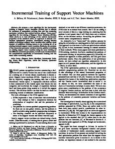
procedure OptMargin set weight u( i ) to be 1 for all examples in X ; r 6 2 ; repeat R choose r examples from X randomly according to u; let ( 
+ 
; ) be a solution of (P1) for R; V the set of violators in X of the solution; if u(V )  u(X )=(3 ) then double the weight u( i ) for all i 2 V ; until V = ; return the last solution; end-procedure.

x

w

x

x

Figure 2. A First Randomized Algorithm The idea is simple. Pick a certain number of examples from X and solve (P1) under the set of constraints corresponding to these examples. We choose examples randomly according to their “weights”, where initially all examples are given the same weight. Clearly, the obtained local solution is, in general, not the global solution, and it does not satisfy some constraints; in other words, some examples are misclassified by the local solution. Then double the “weight” of such misclassified examples, and then pick some examples again randomly according to their weights. If we iterate this process several rounds, the weight of “important examples”, which are support vectors in our case, grows exponentially fast, and hence, they are likely to be chosen. Note that, once all support vectors are chosen at some round, then the local solution of this round is the true one, and the algorithm terminates at this point. By using the Simple Sampling Lemma, we can prove that the algorithm terminates in O(n log m) rounds on average. We describe more precisely the algorithm in Figure 2. We use u there to denote a weight scheme that assigns some integer weight u( i ) to each i 2 X . For this weight scheme u, consider a multiple set U containing each example i exactly u( i) times. Note that U has u(X ) P (= i u( i )) elements. Then by “choose r examples randomly from X according to u”, we mean; to select a set of  examples uniformly at random from all u(rX ) subsets of U. For analyzing the efficiency of this algorithm, we use the Simple Sampling Lemma 1. From it, we can prove the following bound (see [BDW01]).

x x

x x

x

Theorem 2 The average number of iterations executed in the OptMargin algorithm is bounded by 6 ln m = O(n ln m). (Recall that jX j = m and  = n + 1.) We want to apply a similar technique for the nonseparable case. Furthermore, we want to do it in such a way that the only operations acting on the data points are scalar products, and we want the output hyperplane to be defined as a

linear combination of the data points, so that classifying a new point amounts again only to scalar products as operations on data points. The reasons why the formulations in terms of scalar products allow one to use kernels (and thus obtain highly nonlinear actual classifiers) are carefully described in, e.g., [BC00] and [CST00].

3. Alternative Formulations To go on we need an alternative formulation of (P2) given in [BDW01], and based on an intuitive geometric interpretation of (P2) that has been given by Bennett and Bredensteiner [BB00] after the Wolfe dual of (P2). Let Z be the set of composed examples I that are defined as I = ( i1 + i2 +    + ik )=k , with some k distinct elements i1 , i2 , ..., ik of X with the same label (i.e., yi1 = yi2 =    = yik ). The label yI of the composed example I inherits its members’. Throughout this note, we use I for indexing elements of Z and their labels. The def range of I is f1 ::: M g, where M = jZ j; each such I can be identified with ; a set I = fi1  : : : ik g  f1 : : : ng. Note that M  m k . For each I , we use zI to denote the set of original examples from which I is composed. Note also that these composed examples are sort of mass centers of all groups of k homogeneously labeled initial data points. Then the resulting composed examples, for large enough k, may be linearly separable, even if the initial data are not; for instance, in the extreme case where k = m+ (where m+ is the number of positive examples), the set of positive composed examples consists of only one point. (In some unlikely cases a positive composed example might coincide with a negative one; a slight perturbation of the data avoids this case.) We can formulate now:

x

x

x x z

x

x

z

z

z

z

Max Margin for Composed Examples (P5)

w w.r.t. w = (w1 ::: wn), + , and ; , s.t. w  z I  + if yI = 1 and w  zI  ; if yI = ;1: 1

min. k k2 ; (+ ; ; ) 2

We keep the name (P5) for consistency with [BDW01], to ease the comparison of our new algorithm with our previous paper. Note that the combinatorial dimension of (P5) is n + 1, the same as that of (P1). The difference is that we have now M = O(mk ) constraints, which is quite large. On the other hand, except for the margin parameters + and ;, it follows from [BB00] (see also [BDW01]) that the remaining values of the optimal solution (i.e.  ) coincide for (P2) and (P5). This situation is suitable for the sampling technique, and the same algorithm can be applied. Suppose now that we use OptMargin of Figure 2 for solving (P5). Since the combinatorial dimension is the same, we can use r = 6(n + 1)2

w

as before. From our analysis, the expected number of iterations is O(n ln M ) = O(kn ln m). That is, we need to solve QP problems with n + 2 variables and O(n2 ) constraints for O(kn ln m) times. Although this is not bad at all, there are unfortunately some serious problems. The algorithm needs, at least as it is, a large amount of time and space for “book keeping” computation. First of all, we have to keep weights of all M composed examples in Z . Secondly, for finding violators and for modifying weights, we have to go through Z , which takes at least O(M ) steps. Also it is not so easy to choose composed examples randomly according to their weights. Solutions to these problems were obtained in [BDW01], but the proof of the running time of the resulting algorithm depended on an unproven hypothesis. Thus we head towards the main contribution of this paper, a new algorithm, based on a nontrivial geometric lemma, that handles only m weights and avoids searching for violators on all of Z , and at the same time uses only scalar products on data points, so that it combines with any desired kernel. However, before describing it we need to analyze some properties of the solutions of (P5).

4. Properties of the Solutions For a given example set X , let Z be the set of composed  
; ) and (   +  ; ) be the soluexamples. Let (  
+ tions of (P2) for X and (P5) for Z respectively, sharing  as indicated above. Let Xerr
+ and Xerr
; denote respectively the sets of positive and negative outliers. That is, i belongs to Xerr
+ (resp., Xerr
; ) if and only if y i = 1 and   i <
+ (resp., yi = ;1 and   i >
; ). We use `+ and `; to denote respectively the number of positive and negative outliers. From now on, we assume that our constant k is larger than both ` + and `; , and that in fact problem (P5) is linearly separable. Let Xerr = Xerr
+  Xerr
; . The problem (P5) is regarded as the LP-type problem (D  ), where the correspondence is as in (P1) except that Z is used as D here. Let Z0 be a basis of Z . In order to facilitate understanding, we assume nondegeneracy throughout the following discussion. Note that every element of the basis is extreme in Z . Hence, we call elements of Z0 final extremers. By definition, the solution of (P5) for Z is defined by the constraints corresponding to these final extremers. By analyzing the Karush-Kuhn-Tucker (in short, KKT) condition for (P2), in [BDW01] we showed:

w

w x

w

w x

w x

z w z x

Lemma 3 Let I be any positive final extremer, i.e., an element of Z0 such that yI = 1. Then the following properties  . (b) Xerr
+  zI . (c) For every hold: (a)   I = + i 2 zI , if i 62 Xerr
+ , then we have   i =
+ .

x

w x

The corresponding facts hold, mutatis mutandis, for negative final extremers.

procedure ComposedMargin ui 1,2for each i, 1  i  m; r 6 ; loop R0 choose r elements from X randomly according to their weights; R the set of composed examples from Z consisting only of points from R 0; (  +  ; ) the solution of (P5) for R; compute
+ and
; from the local solution; Y the set of points from X ; R0 misclassified by ( 
+ 
; ); check the stopping condition and exit loop if it holds; if u(Y )  u(X )=(3 ) then ui 2ui for each i 2 Y ; end loop; return the last solution ( 
+ 
; ); end procedure.

w

w

x

w

Thus the algorithm first finds a local solution from the sample, and then tests it on all the composed examples. By the previous paragraph, it is partially correct: if it ever stops, the solution it returns is the global solution. It is a very slow algorithm, since at each iteration it runs over all M = mk composed examples. Thus we will not analyze its running time; but its partial correctness as argued will make it easier to argue the correctness of the next algorithm using the second stopping condition. Indeed, the separable problem is on the composed examples but we do not want to scan them all in search for violators, but instead do it on the original data points X . Thus we consider a faster algorithm that runs over the input data points instead, in search of misclassified points: this is the algorithm of Figure 3 with the stopping condition B (we will connect both stopping conditions below): exit the loop if all the points in X ; R 0 are correctly classified (Y = );

Figure 3. A Second Randomized Algorithm

5. New Algorithms Throughout this section, we assume that k is large enough so that the composed examples make up a linearly separable data set; the combinatorial dimension will be now  = k(n + 1) (actually we only need that  upper-bounds the combinatorial dimension; we have also a preliminary argument, that will be described in future work, according to which  = k + n +1). Again X is the set of input data and Z is the set of composed examples. Our algorithms must find a maximal margin separator of these composed examples. Fix a set Z0 of combined examples that is a minimal set of support vectors for the true solution. We will denote by X 0 the set of input points that belong to some composed example in Z0 , so that again jX0 j   . Also note that, again, the solution of the separable maximal margin problem on Z0 is the global solution. Therefore, any local solution that differs from the global solution must misclassify at least one element of Z0 . This is essentially because, by convexity, any locally optimal solution that is globally feasible is globally optimal. Here again misclassification means that the corresponding inequality does not hold. The algorithm in Figure 3 essentially implements the intuition just described. The computation of
+ and
; is made according to lemma 3 (c), by finding the largest distance from to a point i that belongs to a final extremer of the local solution. We use the same template for two algorithms according to two different stopping conditions. Consider first stopping condition A:

w

From Lemma 1, we can bound the expected number of violators as k(n + 1)=r + 1  u(U )  u(U )=(6 ). Again by Markov’s inequality, on average one out of each two iterations will be successful. So it remains to bound the number of successful iterations. By the same argumentation that supports theorem 1 [BDW01], it follows that, as soon as we prove that each successful stage doubles the weight of some point from X 0 , we guarantee the upper bound t < 3 log m on the expected number of rounds. The fact we need to complete the analysis will be a corollary of the proof of the lemma in the next section.

5.1. Equivalence of the Stopping Conditions We prove now that indeed each successful iteration doubles the weight of at least one element of X0 , and that whenever the algorithm of Figure 3 stops (using the stopping condition B), it has found the true optimal solution. We know this holds for stopping condition A, but for B it is not immediate at all, since it is quite different (and cheaper to compute). We prove this fact as a separate geometric lemma. Lemma 4 The stopping conditions are equivalent; i.e., the following two facts are equivalent:

x 2 X ; R0 misclassified by (w
+
;); 2. There exists a composed example z misclassified by (w  +  ; ).

1. There exists

x

classify all composed examples according to (  +  ;); exit the loop if all of them are correctly classified;

w

Proof. Suppose that there is a positive misclassified point p in X ; R0 , the negative case being analogous. This means that  p <
+ . Pick a final extremer 0 of the local solution on composed examples. Its corresponding inequality is tight:  0 = + . Note that lemma 3 applies

x

w x

z

w z

since all composed examples made up from R0 are in R. Thus, it contains all misclassified points in R0, and there are remaining points 2 z0 fulfilling  p =
+ . (The assumption that k is larger than the number of misclassified points is used here.) Construct 1 by replacing one such 2 z0 by p . By linearity,  1 <  0 = + , so 1 is misclassified by (  +  ;). Conversely, let p be a positive composed example misclassified by (  + ;):  p < + . Pick again a final extremer 0 of the local solution. Then we argue first that some misclassified point p , with  p <
+ , is in zp but not in z 0 . Indeed, z0 consists only of points with  
+ . The correctly classified elements of p (if any) have  
+ . Thus, if all misclassified points in zp are accounted for in z0 , we obtain  p   0 = + , which is not the case. Thus, some p 2 zp is misclassified and not in z0 . But, by lemma 3 (b), all misclassified points of R0 are in z0 , and thus p 2 = R0, as was to be shown. tu

x

x

x

z

wx

w

w x

z w z wz

w z

z

w z x w x

z

w x

wz

x

wz

x

x

Finally, we need to argue that at least one point in X0 gets doubled at each nonterminal successful iteration, except the last one. Note first that, if all the composed examples from points in X 0 are correctly classified by the local solution, as we have already said, there can be no misclassified composed examples of Z at all and, by the previous lemma, the algorithm will end. Thus, the composed example p used to start the proof of the lemma (backwards direction) can be actually selected to be composed of points in X0 . Thus, the point p that we find in the proof of the lemma is in X0 , is misclassified, and is not in R0 as the lemma proves. Thus it doubles weight, and this, combined with a more-or-less standard application of Lemma 1, completes the proof. In this way we can obtain:

z

x

Theorem 5 The algorithm in Figure 3, with stopping condition B, obtains the maximal margin hyperplane in less than 6 log m rounds on average. The tail bounds given in [GW00] prove additionally that the probability of deviation from the average is small.

6. Dual Coordinates and our Final Algorithm The dual formulation is obtained by introducing one more variable, the Lagrangian multiplier, for each inequality, i.e. for each data point, differentiating with respect to the primal variables, and equating to zero the derivatives. Thus, the dual variables are coefficients affecting the data points. It can be seen that the dual formulation only needs scalar products among data points, so that a kernel can be used instead; and the outcome defines the hyperplane as a linear combination of data points, so that classifying new points only needs computing scalar products with data

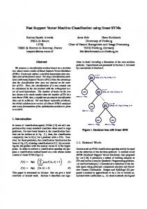
procedure OptMargin set weight u( i ) to be 1 for all examples in X ; r 6 2 ; repeat R choose r examples from X randomly according to u; let ( 
+ 
; ) be a solution of (P2) for R; V the set of violators in X ; R of the solution; if u(V )  u(X )=(3 ) then double the weight u( i ) for all i 2 V ; until V = ; return the last solution; end-procedure.

x

w

x

x

Figure 4. A Last Randomized Algorithm points. Moreover, the optimal value of the Lagrangian multiplier is only nonzero for the support vectors. See [CST00]. We export now the ideas of the previous sections to the dual framework: we first sample, then move into dual form, and then consider composed examples only on the sample (or on their images in feature space). This allows us to introduce a quantity of additional variables (Lagrange multipliers) that is independent of m. Once a local solution is available, the points left unsampled are checked against it, to double the weight of those that led to wrong classifications. Indeed, although it is not fully trivial, it can be seen that all the steps of the algorithm in Figure 3 with stopping condition B can be run only implicitly on the feature space if the kernel is used judiciously. But there is still a somewhat surprising alternative: instead of translating our last algorithm into dual form, we can actually come back to Figure 2! Indeed, by the analysis of [BB00], we know that the optimal  is the same for (P5) and for (P2). Thus, we can simply sample R input data points, solve (P2) on R (in dual form to use kernels), and, according to stopping condition B, check for violators only in X ; R. Thus, we obtain a simple algorithm, Figure 4, which is similar to the one in Figure 2, but without the assumption of separability. Lacking this assumption means we solve (P2) instead of (P1) to find the local solution, since (P1) may well be unfeasible, and then test the local solution only on the unsampled points, since some sampled points actually do violate it. Another subtle difference is the initial value of the constant  , where the dependence of k is hidden. The algorithm in Figure 4 has the same performance guarantees as indicated in the previous theorem, even when the local solution is found in dual form with kernels.

w

7. Conclusions and Further Remarks We have developed here more algorithms for training support vector machines in such a way that we can formally prove rigorous fast convergence results, in the common case

of having larger data sets than the dimension. This continues the research initiated in our previous paper [BDW01]. The advantage of our last algorithm here is the possibility of using it in dual formulation, which is a key to the use of a major feature of support vector machines, namely kernels into feature spaces. The algorithm has been formally proved to have a very mild dependence of the number of data points, although its dependence on the number of outliers for the nonseparable case may become a cause of slow computation. It needs the prior knowledge of a parameter k corresponding to the influence of outliers: all soft margin implementations of SVM need one similar parameter. However, in general there is no clue as to how to choose it, whereas in our case it has a clear intuitive meaning: k must be such that the sets of homogeneously labeled kwise mass-centers are linearly separable, or at least an upper bound on such a value. We have not mentioned experimental validations. Experiments conducted by Norbert Mart´ınez with several variants of our previous algorithms based on the Sampling Lemma indicated that these were competitive with other chunking and decomposition schemas but did not show an spectacular behavior improvement yet. Thus, we have focused on deepening the theoretical understanding of the combinatorial process. Still, we do not think a naive implementation of the algorithm in Figure 5 will be competitive immediately: there is some more work to be done in finding the best possible value of  , where the current bottleneck resides; a lot of care has to be invested in the interaction with the local problem solver, and dedicated data structures allowing fast sampling under the filtered probability distribution could be designed. We can enumerate easily several more issues worth further work. First, there may be other possible ways of analyzing the algorithm in [BDW01]; similarly, there could be other possible ways to analyze our final algorithm here. Second, [GW00] contains other applications of sampling to LP-type problems, some of which look promising for advances in SVMs in case we can map them into dual convex quadratic programming. Third, there is an interesting possibility of not using a true QP subroutine for the local problems, but accepting instead suboptimal solutions: would the sampling rounds make up for this? Overall, we believe that further work may lead to new algorithms with better scaleup properties, applicable to very large datasets with reasonable running times.

References [BDW01] J. L. Balc´azar, Y. Dai, and O. Watanabe, A random sampling technique for training support vector machines, in Proc. Algorithmic Learning Theory (ALT’01), 2001.

[BB00] K. P. Bennett and E. J. Bredensteiner, Duality and geometry in SVM classifiers, in Proc. the 17th Int’l Conf. on Machine Learning (ICML’2000), 57;64. [BC00] K. P. Bennett and C. Campbell, Support Vector Machines: Hype or Hallelujah?, SIGKDD Explorations Newsletter 2, 2 (2000). [BGV92] B. E. Boser, I. M. Guyon, and V. N. Vapnik, A training algorithm for optimal margin classifiers, in Proc. Int. Conf. on Computational Learning Theory (COLT’92), 144–152, 1992. [Lin01] C. J. Lin, On the convergence of the decomposition method for support vector machines, IEEE Trans. on Neural Networks, 2001, to appear. (Also available from http://www.csie.ntu.edu.tw /˜cjlin/papers/.) [CV95] C. Cortes and V. Vapnik, Support-vector networks, Machine Learning 20, 273;297, 1995. [CST00] N. Cristianini and J. Shawe-Taylor, An Introduction to Support Vector Machines, Cambridge University Press 2000. [GW00] B. G¨artner and E. Welzl, A simple sampling lemma: Analysis and applications in geometric optimization, Discr. Comput. Geometry, 2000, to appear. (Also available from http://www.inf.ethz.ch/personal /gaertner/publications.html.) [KG01] S. S. Keerthi and E. G. Gilbert, Convergence of a generalized SMO algorithm for SVM classifier design, Technical Report CD-00-01, Dept. of Mechanical and Production Eng., National University of Singapore, 2000. (Available from http://guppy.mpe.nus.edu.sg /˜mpessk/svm/conv ml.) [LM01] Y.-J. Lee and O. L. Mangasarian, RSVM: Reduced Support Vector Machines, in Proc. First SIAM International Conference on Data Mining, 2001. [Pla99] J. Platt, Fast training of support vector machines using sequential minimal optimization, in Advances in Kernel Methods – Support Vector Learning (B. Scholkopf, C. Burges, and A. J. Smola, eds.), MIT Press, 185;208, 1999. [SBV95] B. Sch¨olkopf, C. Burges, and V. Vapnik, Extracting support data for a given task, in Proc. First Int. Conf. on Knowledge Discovery and Data Mining (KDD’95), 252–257, 1995. [YA00] M.-H. Yang and N. Ahuja, A geometric approach to train support vector machines, in Proc. IEEE Conf. Computer Vision and Pattern Rec., 2000, 430–437.