Fast Online Algorithms for Support Vector Machines Models and Experimental Studies
Vojislav Kecman
Gabriella Melki
Department of Computer Science Virginia Commonwealth University Richmond, USA
[email protected]
Department of Computer Science Virginia Commonwealth University Richmond, USA
[email protected]
Abstract—A novel online, i.e. stochastic gradient, learning algorithm in a primal domain is introduced and its performance is compared to the Sequential Minimal Optimization (SMO) based algorithm for training L1 Support Vector Machines (SVMs) implemented within MATLAB's SVM solver fitcsvm. Their performances are compared on both real and artificial datasets, which contain up to 15,000 samples. These datasets belong to the small and medium class of datasets today. We have shown that classic online learning algorithms implemented in the primal domain can be both extremely efficient and faster up to two orders of magnitude in respect to the SMO algorithm. In particular, unlike the SMO algorithm, our simulations show that the CPU time of OL SVM does not depend on SVM design parameters (penalty parameter C and Gaussian kernel shape parameter σ or on the order of the polynomial kernel). This property is very beneficial for the SVMs' training faced with large and ultra-large datasets. Paper also compares OL SVM with the established stochastic gradient algorithms, Norma and a novel version of an online SVM training algorithm Pegasos dubbed here Pegaz. Keywords—Online learning, Stochastic gradient learning, Training SVM in primal, Support vector machines
I. INTRODUCTION Support Vector Machines (SVMs) are known as both accurate and fast (and consequently very popular) machine learning, i.e. data mining, tools [1-5]. In the original setting, for the so-called L1 SVM, the learning algorithm is based on solving a quadratic programming problem in a dual domain subject to the set of block constraints and a single equality constraint. Historically, this was the leading approach for solving classification and regression tasks by SVMs. Recently several authors have proposed the use of a standard stochastic gradient approach for SVMs while solving machine learning problems [5-8]. The mentioned approaches are extended variants of a classic kernel perceptron algorithm [9]. The main difference between these, otherwise close, approaches presented in [5-8] and in this paper originate from the minimization of slightly different loss (i.e., cost) functions while training the SVM. In [5-8] the cost function was the regularized hinge loss given by (1), while here, both the regularized and unregularized hinge, or soft margin, losses (1) and (2) are minimized. [10] presents the justification for not using the regularization term, 0.5 o
2 2
, shown in (1). We
present two algorithms but the experiments are performed by
978-1-5090-2246-5/16/$31.00 ©2016 IEEE
using only the algorithm which follows from minimizing (2). The two SVM loss functions minimized here are R (o) rhl C
l i 1
max 0, 1 yi o ( xi )
where o( x ) R (o)hl
l i 1
1 2 o , 2 2
max 0, 1 yi o( xi ) ,
l k ( x, x i ) i 1 i
(1) (2)
is the output (the value of an
SVM decision function) for a given input vector x, yi is the label for a sample xi, l is the number of samples i.e., cardinality of the dataset, and C stands for the regularization penalty parameter. The vector containing l outputs to all the training data is o. The SVMs' hinge loss is given in (2) and it is also the first term in (1). The last term on the right hand side of (1) is the regularization term of the hinge loss function. Typically, within the SVM community, this regularization is expressed by squaring the norm of the weight vector w which, geometrically, determines the width of the margin between the two classes. The values of the best parameters αi obtained from minimizing R(o) are same as the ones obtained from minimizing R(w). The penalty parameter C is a trade-off parameter between the size of the margin and the size of the slack variables [1]. The smaller C, the larger the margin creating a more robust classifier. Increasing C to infinity leads to the hard margin classifier, if the data are linearly separable. The proper value of C is not known in advance, and it is obtained by crossvalidation. Indices rhl and hl stand for regularized hinge loss and hinge loss respectively. II. FOUR ONLINE SVMS ALGORITHMS Here the optimal αi values will be obtained by using a classic stochastic gradient descent as follows
i 1 i i
R , i
(3)
where R is given by (1) i.e., (2) and ηi is a learning rate defining the stepsize at each iteration. We will present two algorithms as given in [5-8] first. In both cases, the decision function or, the output o, of SVM for a given input vector x is expressed as a kernel expansion o( x )
l k ( x, xi ) . i 1 i
(4)
Note that o is obtained without use of the bias term b which is not needed for positive definite kernels. (It is straightforward to expand the algorithms shown below with the bias b. See equations (6) and (7)). Next, the minimization of loss functions is done in a stochastic way, meaning the value of the expansion parameter αi will be updated after a single sample is presented. In other words, the gradients of R will be calculated without the summation over all data samples. Under such a stochastic update, the stochastic gradient descent for updating expansion coefficients αi is given in [5-6], and called Naïve Online R Minimization Algorithm (NORMA). A slightly different learning algorithm is proposed in [7-8]. In [7], it is originally dubbed PEGASOS (standing for Primal Estimated sub-GrAdient SOlver for SVM). Both algorithms are shown below. The viol variable denotes the violator, i.e. the sample which lies on the wrong side of a separation boundary. LIST 1: NORMA ONLINE ALGORITHM Minimization of Rrhl in (1) Set I 1: l & define number of epochs N Shuffle the dataset & Initialize α 0, i 0 for t 1, , Nl
C 2/t i i 1, if i l , i 0, end viol yi k ( x i ,:) * α I not i I i , α( I not i ) 1 / C α( I not i )
if viol 1 i yi end end .
LIST 2: PEGAZ ONLINE ALGORITHM Minimization of Rrhl in (1) Define the number of epochs N Shuffle the dataset & Initialize α β 0, i 0 for t 1, , Nl
C 2/t i i 1, if i l , i 0, end α β viol yi k ( xi ,:) * α if viol 1
i i yi end end α β. k(xi, :) is the i-th row of the Gramm matrix of corresponding kernel. It contains the values of i-th kernel at all the other data points. k(:, xi) is then a transposed k(xi, :) meaning a column vector with same entries as k(xi, :).
We have christened the algorithm in List 2 as Pegaz for the sake of differentiating between four SVM learning algorithms used here. Pegasos was the name given by same author to a similar stochastic gradient procedure in [7]. Here, the projection step from Pegasos is missing and the lines in List 2 are equal to the ones in [8]. Hence, the name just connects to the origin of the algorithm. As with all numerical iterative algorithms, there are several iteration hyperparameters one has to configure. The first variable to define in stochastic gradient descent procedures is the learning rate η. In the lists above, we have accepted the suggestion about the 'optimal stepsize' η as given in [11]. This choice is different but 'similar' to the suggestions given in [5-8]. Another important decision is setting how many iterations one will perform. They are defined by the number of epochs. While there are no clear guidelines, a rule of thumb would suggest that the bigger the datasets, the smaller the number of epochs should be. More about this issue can be found in our companion paper at the conference [12]. There is also an open issue on how to choose the final expansion parameter vector α. In [7] and [8], it is suggested to cache all the alpha updates, and then take the average as the final value of vector α. In [12], several strategies have been explored to define the final vector of expansion parameters α. More about this issue can be found there, but the overall suggestion is that taking the average over all the αi stored may not always be the best strategy. However, there is a more important point concerning the two online SVM algorithms shown. They use stochastic gradient descent for a minimization of Rrhl given in (1) and they should result in same final values of alpha vectors' entries, assuming that other simulation specifications (learning rate and order of data points selected) are equal. This is the case only if one makes a single pass through the dataset (number of epochs N = 1). For N > 1, they result in different solutions and neither the number of support vectors (data points having |αi| value > 0) nor the αi values are equal. An extensive experimental comparison on various datasets may give an answer to the question which of the two might be more preferable. This is not on our agenda here. Here, we have devised algorithms based on stochastic gradient for training SVMs minimizing both loss functions shown, namely (1) and (2). However, all our experimental comparisons are done by the model of the soft margin loss shown in List 3b. This is similar to the approach for the kernel perceptron learning algorithm given in [9], but we use the SVM's soft margin loss (2) here. In addition to being very simply structured, our OL SVM algorithms CPU time efficiency is improved by calculating viol variable with the help of caching the output vector o only when there is a violation, i.e., an αi update. Such a calculation of viol is much more efficient than the way is done in Lists 1 and 2. Namely, by using output vector o one avoids computing a dot product of l-dimensional vectors in each iteration step. Such a speedup by using the output o can be implemented in Norma and Pegaz algorithms too, but this is not how they have been originally introduced. Finally, all four algorithms, after calculating the expansion vector α, have designed the SVM model which for every new input vector x makes the following decision
o( x ) sign
l k ( x, x i ) i 1 i
.
(5)
LIST 3A: SVM ONLINE ALGORITHM (OL SVM) FOR RRHL Minimization of Rrhl in (1) Define the number of epochs N Shuffle the dataset & Initialize α 0, o 0, i 0 for t 1, , Nl
in List 3b. Hence, we present comparisons of OL SVM with the SMO based algorithm within the MATLAB environment first.( SMO is the most popular training algorithm for SVMs and it stands for Sequential Minimal Optimization [13]). MATLAB has recently implemented it within the routine fitcsvm [14]. The first batch of simulations and comparison results in section III are obtained by comparing the performances of OL SVM and fitcsvm. Then, we'll compare three online SVM algorithms given in the lists above. III. DATASETS AND RESULTS
C 2/t
Paper presents comparisons of two binary SVM classifiers the SMO based fitcsvm and our implementation of OL SVM, on datasets that contain up to 15,000 samples. Basic information about the datasets used are presented in Table 1.
i i 1, if i l , i 0, end viol yi oi if viol 1 o o yi i / C k :, xi
TABLE I.
i 1 / C i yi if viol 1 o o i k :, xi / C
i 1 / C i
DATASETS BASIC INFORMATION
Dataset
# Samples
# Features
cancer
198
32
sonar
208
60
vote
232
16
2,427
20
eukaryotic
end end .
LIST 3B: SVM ONLINE ALGORITHM (OL SVM) FOR RHL
prototask
8,192
21
reuters
11,069
8,315
chess board data Two normally distributed classes
8,000
2
15,000
2
Minimization of Rhl in (2) Define the number of epochs N Shuffle the dataset & Initialize α 0, o 0, i 0 for t 1, , Nl
C 2/t i i 1, if i l , i 0, end viol yi oi if viol 1 o o yi k (:, xi )
i i yi end end .
Note that the bias term b is not needed when positive definite kernels are implemented, but it can be used. In this case, whenever viol < 1 the b is updated by (6). Also, and only when viol < 1, the term ηyj must be added to the right hand side of the output o in Lists 3. The bias updates and the SVM model output o are given in (6) and (7). b b yi , o( x )
l k ( x, x i ) b i 1 i
(6) .
(7)
The main task in this paper is to experimentally investigate the potential of the kernel perceptron like OL SVM algorithm obtained by minimizing the soft margin loss Rhl (2) and given
Data which originally are not binary have been transformed into binary classification problem by grouping the samples into two classes. For the eukaryotic dataset, results are shown for classifying class 4 vs the rest. The prototask dataset is transformed into a balanced two class problem, where if yi >= 89 xi is assigned to class 1, otherwise, the data belongs to class 2. In all simulations, the SVM with a Gaussian kernel have been used. The results shown are obtained by performing the 5fold cross-validation. The two design hyper-parameters have been used out of the following range of parameters. The penalty parameter C has been chosen as 9 values in the span from C = 1e-4 to C = 1e4. The Gaussian kernel shape parameter σ is different for each dataset. Typically, it is in the range [1e-1 1e0 1e1 1e2]. Such a set of, usually, 9 C and 4 σ values would lead to 36*5 = 180 runs for each dataset which can really be computationally expensive for bigger datasets. For example, the SMO algorithm based fitcsvm neded 2.7 days to finish the cross-validation runs for reuters data. Table II shows the average error rates of SMO (in MATLAB's fitcsvm implementation) and OL SVM on test datasets. OL SVM is more accurate than fitcsvm for all but one dataset. In all runs OL SVM is faster than SMO. With the increase in datasets size, the speedup significantly increases. Even more important is that SMO based fitcsvm training time sharply increases with both a bad conditioning of kernel matrix K (say, for broad Gaussian kernels or higher order polynomial ones) and big penalty parameter C. Here proposed OL SVM training time doesn't depend upon these hyperparameters.
TABLE II.
AVERAGE ERROR RATE AND SPEEDUP OF OL SVM VS. SMO
Dataset
Error Rate SMO, %
Error Rate OL SVM, %
cancer
24.00
25.62
OL SVM is that time faster 4.1
sonar
34.70
24.35
3.68
vote
22.68
8.09
1.89
eukaryotic, 4 vs rest
36.05
14.55
5.67
prototask
33.57
11.28
5.61
reuters
5.65
4.48
4.10
chess board data Two normally distributed classes
13.62
4.27
7.65
28.25
7.82
41.50
shown a known weakness of having long CPU training time for large values of both C and σ. There are two reasons for this. SMO is a kind of two coordinate descent, iterative algorithm which, for broad Gaussian kernels, iterates slowly to the bottom of cost function Rrhl, along the 'badly conditioned' valleys, or to the box defined by C value. For a large C value, the box limits are very far from the origin, and one needs a lot of steps to reach them. On the other hand, the OL SMO is not influenced very much by the hyper-parameters values. Its CPU time is determined primarily by the number of iterations, which is defined by datasets cardinality and number of epochs N defined before the calculation. Figs 3 and 4 show the performances of SMO and OL SVM for the reuters data. This is a very sparse dataset (only 11,069 samples in 8,315 dimensional space). The curves in all simulation have a typical sew-saw behavior due to the order of selection of C and σ. Typically, one C is selected and it is being combined with all the shape parameters given. The last runs are with the largest values of C and σ.
Fig. 1. Error rates of SMO and OLSVM algorithms for two normally distributed classes in 2-dimensional space. Number of samples is 15,000
Fig. 3. Error rates of SMO and OLSVM algorithms for reuters dataset in 8,315-dimensional space. Number of samples is 11,069.
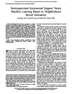
Fig. 2. CPU times of SMO and OLSVM algorithms for two normally distributed classes in 2-dimensional space. Number of samples is 15,000
Figs 1 and 2 show the typical and characteristic changes of error rates and CPU time for the two methods in 24 crossvalidation runs (6 C and 4 σ values). For all datasets used here, the SMO based algorithm implemented in fitcsvm code has
Fig. 4. CPU times of SMO and OLSVM algorithms for reuters dataset in 8,315-dimensional space. Number of samples is 11,069.
Next set of results shows the comparisons of the three stochastic gradient SVM algorithms introduced in section II (Norma, Pegaz and OL SVM from List 3b) in our MATLAB implementation, on the chess board data containing 4,992 samples. Figs 5 and 6 show the performances of the original algorithms given in the lists. Note that the Pegaz algorithm shown in List 2 does not include the projection step introduced in [7] for Pegasos. It is the stochastic algorithm from [8].
In Figs. 7 and 8, all three algorithms are compared by using the same method of calculating violators as presented in List 3b for the here proposed OL SVM. This sped up Norma and Pegaz as it can be seen in Fig. 8, but OL SVM is still faster and more accurate than the other two stochastic gradient algorithms.
Fig. 7. Error rates of OLSVM, Norma and Pegaz algorithms for chessboard dataset in 2-dimensional space. Number of samples is 4,992. Violators are calculated as shown in the List 3b. Fig. 5. Error rates of OLSVM, Norma and Pegaz algorithms for chessboard dataset in 2-dimensional space. Number of samples is 4,992. Performances of original algorithms given in the lists.
While the error rate of Norma and OL SVM are similar, OL SVM is 2 times faster than Norma and 4 times faster than Pegaz, in our implementations of the original algorithms. Pegaz’ error rates are higher than the ones shown by the other two online SVM algorithms.
Fig. 8. CPU times of OLSVM, Norma and Pegaz algorithms for chessboard dataset in 2-dimensional space. Number of samples is 4,992. Violators are calculated as shown in the List 3b.
IV.
Fig. 6. CPU times of OLSVM, Norma and Pegaz algorithms for chessboard dataset in 2-dimensional space. Number of samples is 4,992. Performances of original algorithms given in the lists.
CONCLUSIONS
The paper introduces two new stochastic gradient based SVM learning algorithms in primal dubbed OL SVM. The learning classification algorithms are devised and shown in Lists 3a and 3b as described next. The algorithm which minimizes a soft margin (a.k.a. hinge) loss without the quadratic regularization term Rhl (2) is presented in List 3b and used for comparisons with other SVM models. This approach has some similarities with the kernel perceptron learning
algorithm expressed in dual variables. In List 3a, we also present the stochastic gradient based algorithm for SVM which minimizes the regularized hinge loss Rrhl (1). In addition, the two known online algorithms NORMA and a variant of Pegasos dubbed PEGAZ are also shown and used in experiments.
to the training CPU times shown by the SMO algorithm, which slows down significantly due to worse conditioning of Hessian matrix used in a dual space.
The first set of experiments compares OL SVM with the classic and most popular SVM training approach, the SMO algorithm. All the experiments have been performed in MATLAB and they show the superiority of OL SVM in terms of both accuracy and CPU time needed for performing the 5fold cross-validations on various data. The comparisons have been performed on several binary classification datasets, with up to 15,000 samples. Whether this superiority claim is right and valid for the implementation of the two algorithms on other platforms (C++, Java, Python, R) is partly answered in a companion paper [12] and it is still the subject of present, as well as it will be of the future, investigations by using more datasets of various sizes and characteristics.
[1]
Next set of experiments shows the performance comparisons of three stochastic gradient algorithms given in the Lists 1, 2 and 3b (Norma, Pegaz and OL SVM) on the twodimensional chessboard dataset with 4,992 samples. OL SVM has shown superiority in respect to the other two online methods. It needs less CPU time and it achieves higher accuracy than Norma and Pegaz. These results should be considered as the preliminary ones but they hint that OL SVM is highly likely very powerful algorithm. Our future work will be focused on implementing both OL SVM algorithms (shown in Lists 3a and 3b) in C++ and make them suitable to work with much larger datsets. The initial results presented in the companion paper at the conference [12], are promising. An important characteristic of OL SVM is that the CPU time needed for the training does not depend upon the values of penalty parameter C or on the kernel hyperparameter values (shape parameter of Gaussian kernel or the order of the polynomial one). This feature significantly reduces the OL SVM training time for bigger values of both C and Gaussian shape parameters (i.e., for higher order polynomials) compared
REFERENCES
[2] [3]
[4]
[5] [6] [7]
[8]
[9] [10] [11] [12]
[13]
[14]
Vapnik V., The Nature of statistical learning theory, Springer-Verlag, 1995. Cortes C. and Vapnik V., Support-vector networks, Machine Learning, 20(3), 1995, pp. 273–297. Kecman V., Vogt M., Huang T-M., On the Equality of Kernel AdaTron and Sequential Minimal Optimization in Classification and Regression Tasks and Alike Algorithms for Kernel Machines, Proc. of the 11th European Symposium on Artificial Neural Networks, ESANN 2003, Bruges, Belgium, 2003, pp. 215 – 222. Huang T.-M., V. Kecman, I. Kopriva, Kernel based algorithms for mining huge data sets, supervised, semi-supervised, and unsupervised learning, Springer-Verlag, Berlin, Heidelberg, 2005. Schoelkopf B., Smola A. J., Learning with Kernels - Support Vector Machines, Regularization, Optimization, and Beyond, MIT Press, 2002. Kivinen J., Smola A. J., Williamson R. C., Large Margin Classification for Drifting Targets, Neural Information Processing Systems, 2002. Shalev-Shwartz, Y. Singer, and N. Srebro. Pegasos: Primal estimated subgradient solver for SVM. In Proc. 24th Intl. Conf. on Machine Learning (ICML’07), pp. 807–814. ACM, 2007. S. Shalev-Shwartz and S. Ben-David, Understanding Machine Learning From Theory to Algorithms. New York: Cambridge University Press, 2014. Herbrich R., Learning Kernel Classifiers - Theory and Algorithms, The MIT Press, 2002. Collobert R., Bengio S., Links between Perceptrons, MLPs and SVMs, Proc. of the 21st Intl. Conf. on Machine Learning, Banff, Canada, 2004 Ben-Taly A., Nemirovski A., Lectures on modern convex optimization, 2013. Melki G., Kecman V., Speeding-Up On-Line Training of L1 Support Vector Machines, Submitted to IEEE SoutheastConf, Norfolk, VA, 2016. Platt J. C., Sequential Minimal Optimization, A Fast Algorithm for Training Support Vector Machines, Microsoft Research, Technical Report MSR-TR-98-14, 1998 MathWorks: http://www.mathworks.com/help/stats/fitcsvm.html, 2014