Pseudodynamic tests on a large-scale model of an ...

EUROPEAN COMMISSION JOINT RESEARCH CENTRE

Institute for the Protection and Security of the Citizen European Laboratory for Structural Assessment (ELSA) I-21020 Ispra (VA), Italy

Pseudodynamic tests on a large-scale model of an existing RC bridge using non-linear substructuring and asynchronous motion A. Pinto, P. Pegon,G. Magonette, J. Molina, P. Buchet, G. Tsionis

2002

EUR 20525 EN

LEGAL NOTICE Neither the European Commission nor any person acting on behalf of the Commission is responsible for the use which might be made of the following information.

A great deal of additional information on the European Union is available on the Internet. It can be accessed through the Europa server (http://europa.eu.int)

EUR 20525 EN © European Communities, 2002 Reproduction is authorised provided the source is acknowledged Printed in Italy

Pseudodynamic tests on an existing RC bridge using non-linear substructuring and asynchronous motion

CONTENTS List of figures .....................................................................................................................iii List of tables ...................................................................................................................... vii Aknowledgements .............................................................................................................. ix Abstract............................................................................................................................... xi 1. INTRODUCTION ....................................................................................................... 1 2. DESIGN OF THE MODELS AND TEST SET-UP ................................................... 2 2.1. Geometric characteristics and material properties............................................... 2 2.2. Instrumentation.................................................................................................... 5 2.3. Application of the vertical load ........................................................................... 5 3. THE PSEUDODYNAMIC TESTING METHOD WITH SUBSTRUCTURING...... 6 3.1. Pseudodynamic testing of large-scale structures ................................................. 6 3.2. The α-Operator Splitting scheme......................................................................... 6 3.3. The substructuring technique .............................................................................. 9 3.4. Substructuring in the case of asynchronous motion ............................................ 9 3.5. The continuous pseudodynamic testing with non-linear substructuring ........... 10 3.6. Implementation for the Talübergang Warth Bridge tests .................................. 13 4. NUMERICAL MODELS FOR THE SUBSTRUCTURED PIERS ......................... 14 4.1. The Fibre/Timoshenko Beam element in Cast3m ............................................. 14 4.2. Alternative models for the cross-section ........................................................... 15 4.2.1. The equivalent I cross-section ................................................................... 16 4.2.2. New elements implemented in Cast3m ..................................................... 17 4.3. Alternative models for the beam element.......................................................... 17 4.4. Calibration on the basis of cyclic tests .............................................................. 18 5. PRE-TEST NUMERICAL SIMULATION OF THE PSD TESTS .......................... 21 5.1. Description of the model ................................................................................... 21 5.2. Damping matrix................................................................................................. 23 5.3. Modal analysis................................................................................................... 24 5.4. Input motion ...................................................................................................... 24 5.5. Numerical simulation of the PSD tests.............................................................. 25 6. PSEUDODYNAMIC TESTING OF THE BRIDGE MODEL................................. 26 6.1. Control and data acquisition set-up ................................................................... 26 6.2. Check tests......................................................................................................... 27 6.3. Low-level earthquake test.................................................................................. 28 6.4. Nominal earthquake test .................................................................................... 29 6.5. High-level earthquake test ................................................................................. 30 6.6. Seismic assessment of the bridge ...................................................................... 31 6.6.1. Deformation and curvature of the physical piers....................................... 31 6.6.2. Relation between drift and displacement ductility .................................... 31 6.6.3. Damage assessment ................................................................................... 32 6.6.4. Overall damage index................................................................................ 34 6.6.5. Vulnerability functions .............................................................................. 35 6.7. Final collapse test – effect of cycling ................................................................ 36 7. SUMMARY AND CONCLUSIONS........................................................................ 37 REFERENCES .................................................................................................................. 38 ANNEX A: FIGURES ...................................................................................................... 43 ANNEX B: PHOTOGRAPHIC DOCUMENTATION .................................................... 77 ANNEX C: CONSTRUCTION DRAWINGS .................................................................. 95 ANNEX D: INSTRUMENTATION ............................................................................... 105

i


ii


LIST OF FIGURES Figure 1. Talübergang Warth Bridge................................................................................... 1 Figure 2. Parallel procedures: simple inter-field procedure (a), improved inter-field procedure (b) and intra-field procedure..................................................................... 12 Figure 3. PSD test with substructuring for the Talübergang Warth Bridge ...................... 13 Figure 4. Dimensions of the scaled (1:2.5) pier cross-section........................................... 15 Figure 5. Discretisation of alternative models for the cross-section ................................. 16 Figure 6. Equilibrium of forces in diagonally cracked element ........................................ 18 Figure 7. Dimensions of the scaled deck cross-section ..................................................... 21 Figure A1. Pier A20, force-displacement for alternative models...................................... 45 Figure A2. Pier A20, moment-curvature for alternative models....................................... 45 Figure A3. First ten eigenmodes of the bridge from numerical model (top: vertical, bottom: horizontal) .................................................................................................... 46 Figure A4. Pier A40, force-displacement (blue: fibre model with reduced steel, red: damage model, green: fibre model with applied moment)........................................ 46 Figure A5. Pier A20, force-displacement (blue: fibre model (-60% steel), red: damage model)........................................................................................................................ 47 Figure A6. Pier A20, absorbed energy (blue: fibre model (-60% steel), red: damage model)........................................................................................................................ 47 Figure A7. Pier A30, force-displacement (blue: fibre model (-60% steel), red: damage model)........................................................................................................................ 48 Figure A8. Pier A30, absorbed energy (blue: fibre model (-60% steel), red: damage model)........................................................................................................................ 48 Figure A9. Pier A40, force-displacement (blue: fibre model (-60% steel), red: damage model)........................................................................................................................ 49 Figure A10. Pier A40. Absorbed energy (blue: fibre model (-60% steel), red: damage model, black: experimental) ...................................................................................... 49 Figure A11. Pier A50, force-displacement (blue: fibre model (-65% steel), red: damage model)........................................................................................................................ 50 Figure A12. Pier A50, absorbed energy (blue: fibre model (-65% steel), red: damage model)........................................................................................................................ 50 Figure A13. Pier A60, force-displacement (blue: fibre model (-70% steel), red: damage model)........................................................................................................................ 51 Figure A14. Pier A60, absorbed energy (blue: fibre model (-70% steel), red: damage model)........................................................................................................................ 51 Figure A15. Pier A70, force-displacement (blue: fibre model, red: damage model, black: experimental) ............................................................................................................. 52 Figure A16. Pier A70, Absorbed energy (blue: fibre model, red: damage model, black: experimental) ............................................................................................................. 52 Figure A17. Input accelerograms (a) Abutment ABW, (b) Pier A20, (c) Pier A30, (d) Pier A40, (e) Pier A50, (f) Pier A60, (g) Pier A70, (h) Abutment ABG .......................... 53 Figure A18. Acceleration response spectra (a) Abutment ABW, (b) Pier A20, (c) Pier A30, (d) Pier A40, (e) Pier A50, (f) Pier A60, (g) Pier A70, (h) Abutment ABG .... 54 Figure A19. Force-displacement. (a) Pier A20, (b) Pier A30, (c) Pier A40, (d) Pier A50, (e) Pier A60, (f) Pier A70 (blue: numerical PSD - αOS, red, numerical PSD – implicit). .................................................................................................................... 55 Figure A20. Force-displacement for low-level (0.4xNE) earthquake, pre-test numerical simulation αOS (a) Pier A20, (b) Pier A30, (c) Pier A40, (d) Pier A50, (e) Pier A60, (f) Pier A70................................................................................................................ 56

iii


Figure A21. Force-displacement for nominal (1.0xNE) earthquake, pre-test numerical simulation αOS (a) Pier A20, (b) Pier A30, (c) Pier A40, (d) Pier A50, (e) Pier A60, (f) Pier A70 ................................................................................................................57 Figure A22. Force-displacement for high-level (2.0xNE) earthquake, pre-test numerical simulation αOS (a) Pier A20, (b) Pier A30, (c) Pier A40, (d) Pier A50, (e) Pier A60, (f) Pier A70 ................................................................................................................58 Figure A23. Force-displacement for low-level (0.4xNE) earthquake – experimental results, (a) Pier A20, (b) Pier A30, (c) Pier A40, (d) Pier A50, (e) Pier A60, (f) Pier A70.............................................................................................................................59 Figure A24. Displacement history for low-level (0.4xNE) earthquake, (a) Pier A20, (b) Pier A30, (c) Pier A40, (d) Pier A50, (e) Pier A60, (f) Pier A70 (solid line: pre-test numerical simulation, dotted line: experimental) ......................................................60 Figure A25. Evolution of Park & Ang Damage Index for low-level (0.4xNE) earthquake, (a) Pier A20, (b) Pier A30, (c) Pier A40, (d) Pier A50, (e) Pier A60, (f) Pier A70...61 Figure A26. Force-displacement for nominal (1.0xNE) earthquake – experimental results, (a) Pier A20, (b) Pier A30, (c) Pier A40, (d) Pier A50, (e) Pier A60, (f) Pier A70...62 Figure A27. Displacement history for nominal (1.0xNE) earthquake, (a) Pier A20, (b) Pier A30, (c) Pier A40, (d) Pier A50, (e) Pier A60, (f) Pier A70 (solid line: pre-test numerical simulation, dotted line: experimental) ......................................................63 Figure A28. Evolution of Park & Ang Damage Index for nominal (1.0xNE) earthquake, (a) Pier A20, (b) Pier A30, (c) Pier A40, (d) Pier A50, (e) Pier A60, (f) Pier A70...64 Figure A29. Force-displacement for high-level (2.0xNE) earthquake – experimental results, (a) Pier A20, (b) Pier A30, (c) Pier A40, (d) Pier A50, (e) Pier A60, (f) Pier A70.............................................................................................................................65 Figure A30. Displacement history for high-level (2.0xNE) earthquake, (a) Pier A20, (b) Pier A30, (c) Pier A40, (d) Pier A50, (e) Pier A60, (f) Pier A70 (solid line: pre-test numerical simulation, dotted line: experimental) ......................................................66 Figure A31. Evolution of Park & Ang Damage Index for high-level (2.0xNE) earthquake, (a) Pier A20, (b) Pier A30, (c) Pier A40, (d) Pier A50, (e) Pier A60, (f) Pier A70...67 Figure A32. Damage pattern for Pier A40, low-level (0.4xNE) earthquake .....................68 Figure A33. Damage pattern for Pier A40, nominal (1.0xNE) earthquake .......................68 Figure A34. Damage pattern for Pier A40, Final collapse test..........................................69 Figure A35. Damage pattern for Pier A70, high-level (2.0xNE) earthquake ....................69 Figure A36. Shear (solid line) and flexural (dashed line) deformation. (a) pier A70, lowlevel (0.4xNE) earthquake, (b) pier A70, nominal (1.0xNE) earthquake, (c) pier A70, high-level (2.0xNE) earthquake, (d) pier A40, low-level (0.4xNE) earthquake, (r) pier A40, nominal (1.0xNE) earthquake, (f) pier A40, high-level (2.0xNE) earthquake ..................................................................................................................70 Figure A37. Evolution of curvature along the height of the piers. (a) pier A70, low-level (0.4xNE) earthquake, (b) pier A70, nominal (1.0xNE) earthquake, (c) pier A70, high-level (2.0xNE) earthquake, (d) pier A40, low-level (0.4xNE) earthquake, (r) pier A40, nominal (1.0xNE) earthquake, (f) pier A40, high-level (2.0xNE) earthquake ..................................................................................................................71 Figure A38. Drift demand – displacement ductility, experimental results ........................72 Figure A39. Maximum horizontal displacement of the deck ............................................72 Figure A40. Drift demand for the bridge piers ..................................................................73 Figure A41. Displacement ductility demand for the piers.................................................73 Figure A42. Distribution of dissipated energy in the bridge piers.....................................74 Figure A43. Vulnerability function: Park and Ang Damage Index – earthquake intensity ....................................................................................................................................74

iv


Figure A44. Vulnerability function: Drift demand – earthquake intensity ....................... 75 Figure A45. Vulnerability function: Displacement ductility – earthquake intensity ........ 75 Figure A46. Vulnerability function: Normalised stiffness – earthquake intensity............ 76 Figure A47. Short pier A70: Park and Ang Damage Index – earthquake intensity .......... 76 Figure B1. Talübergang Warth Bridge in Austria (both independent lanes are shown) ... 79 Figure B2. Construction of the specimens: formwork of the base block (a), lower part of the pier shaft (b), casting of concrete at 13 m (c) and general view of the finished pier models (d)........................................................................................................... 79 Figure B3. Transportation of the model of the short pier A70 inside the lab.................... 80 Figure B4. Piers in the lab before testing: view from the north side with instrumentation and reference frames (a) and view from the east side (b).......................................... 81 Figure B5. Short pier A70: application of vertical and horizontal loads........................... 82 Figure B6. Tall pier A40: application of vertical and horizontal loads............................. 82 Figure B7. Actuator controllers ......................................................................................... 83 Figure B8. Acquisition of instrumentation data ................................................................ 83 Figure B9. On-line visualisation of data from controllers and instrumentation measurements ............................................................................................................ 84 Figure B10. Computers running the PSD algorithm and non-linear numerical models for the substructured piers. .............................................................................................. 84 Figure B11. Pier A40, Damage pattern at North face after the Low-level earthquake ..... 85 Figure B12. Pier A40, Damage pattern at West face after the Low-level earthquake ...... 85 Figure B13. Pier A40, Damage pattern at East face after the Low-level earthquake........ 86 Figure B14. Pier A40, Damage pattern at South-East face after the Low-level earthquake ................................................................................................................................... 86 Figure B15. Hysteresis loops for substructured piers A20 and A30 for the nominal earthquake.................................................................................................................. 87 Figure B16. On-line comparison of experimental and pre-test displacement histories for the nominal earthquake.............................................................................................. 87 Figure B17. Pier A40, Damage pattern at North face after the High-level earthquake..... 88 Figure B18. Pier A40, Damage pattern at East face after the High-level earthquake, detail at 3.5 m ...................................................................................................................... 89 Figure B19. Pier A70, Damage pattern at North face after the High-level earthquake..... 89 Figure B20. Pier A70, Damage pattern at South face after the High-level earthquake, note the vertical cracking in correspondence to the longitudinal reinforcement............... 90 Figure B21. Pier A70, Damage pattern at West face after the High-level earthquake...... 90 Figure B22. Pier A70, Rupture of longitudinal rebar during the High-level earthquake .. 91 Figure B23. Pier A40, Damage pattern at North face after the final cyclic test................ 91 Figure B24. Pier A40, Damage pattern at South face after the final cyclic test................ 92 Figure B25. Pier A40, Damage pattern at East face after the final cyclic test .................. 93 Figure B26. Pier A40, Buckling of longitudinal reinforcement at 3.5m ........................... 94 Figure C1. Vertical reinforcement of pier A70 (side view) .............................................. 97 Figure C2. Vertical reinforcement of pier A70 (sections A-A, B-B) ................................ 98 Figure C3. Vertical reinforcement of pier A70 (sections C-C, D-D) ................................ 99 Figure C4. Horizontal reinforcement of pier A70 ........................................................... 100 Figure C5. Vertical reinforcement of pier A40 (side view) ............................................ 101 Figure C6. Vertical reinforcement of pier A40 (sections A-A, B-B) .............................. 102 Figure C7. Vertical reinforcement of pier A40 (sections C-C, D-D) .............................. 103 Figure C8. Horizontal reinforcement of pier A40 ........................................................... 104 Figure D1. Pier A70 general side view of the instrumentation ....................................... 107 Figure D2. Pier A70, numbering of diagonal LVDTs..................................................... 107

v


Figure D3. Pier A70, numbering of inclinometers ..........................................................108 Figure D4. Pier A70, numbering of side vertical LVDTs................................................108 Figure D5. Pier A40, general side view of the instrumentation.......................................109 Figure D6. Pier A40, numbering of diagonal LVDTs .....................................................110 Figure D7. Pier A40, numbering of inclinometers ..........................................................111 Figure D8. Pier A40, numbering of side vertical LVDTs................................................111

vi


LIST OF TABLES Table 1. Similitude relationship between the full-scale prototype (P) and the constructed model (M) .................................................................................................................... 3 Table 2. Geometrical properties of the specimens and seismic code requirements ............ 4 Table 3. Concrete mechanical properties for the physical piers (average values) .............. 4 Table 4. Steel mechanical properties for the physical piers (average values)..................... 4 Table 5. Material properties .............................................................................................. 14 Table 6. Characteristics for different models .................................................................... 17 Table 7. Absorbed energy (kNm) ...................................................................................... 19 Table 8. Values of force and displacement for the bridge piers ........................................ 20 Table 9. Vertical steel areas (cm2) for the substructured piers.......................................... 20 Table 10. Geometric properties of the deck cross-section................................................. 21 Table 11. Eigenfrequencies of Talübergang Warth Bridge (1[Flesch et al., 1999], 2[Flesch et al., 2000])............................................................................................................... 24 Table 12. Number of points for different phases of each step and error energy (kNm).... 27 Table 14. Damage of the bridge piers ............................................................................... 32 Table 15. Maximum drift and ductility demands for the piers.......................................... 32 Table 16. Energy dissipated by the bridge piers (% of total) ............................................ 33 Table 17. Park and Ang Damage Index............................................................................. 33 Table 18. Normalised stiffness .......................................................................................... 33 Table 19. Overall Park and Ang Damage Index................................................................ 35 Table 20. Displacement ductility and drift capacities for the cyclic and PSD tests .......... 36

vii


viii


AKNOWLEDGEMENTS The successful completion of the tests of the VAB Bridge results from the cooperation of the VAB project partners: arsenal (project coordinator), ISMES, University of Porto, ICTP, CIMNE and SETRA, as well as from the work performed by the ELSA staff, namely: F. Taucer, A. Colombo and P. Negro for the design and control of the construction; P. Tognoli, O. Hubert and M. Drago for instrumentation, mounting of control and measurement equipment; J. Esteves and A. Zorzan for the model transportation and mounting of the loading devices. The Vulnerability Assessment of Bridges (VAB)1 project was financed by the European Commission, DG XII, Environment and Climate Programme, Contract No. ENV4-CT970574, project officer: M. Yeroyanni. G. Tsionis is a JRC grant holder, Contract No. 15775-2000-03 P1B20 ISP IT, financed by the SAFERR Research Network, CEC Contract No. HPRN-CT-1999-00035.

1

http://www.arsenal.ac.at/vab/encp02.htm.

ix


x


ABSTRACT Within the VAB research program, pseudodynamic tests on a large-scale model of an existing bridge were carried out in the reaction wall of the ELSA laboratory of the Joint Research Centre, applying the substructuring method. Asynchronous input motion, generated for the bridge site, was considered at the base of the piers and abutments. Nonlinear substructuring was successfully implemented for the first time at world level by considering appropriate hysteretic models for the substructured piers. Pre-test numerical calculations were carried out in order to define the simplest, yet accurate analytical models for the substructured piers. The results of cyclic tests on largescale specimens and refined analyses were used to calibrate the models for the numerical piers. The pseudodynamic test was simulated numerically and the results were compared to the experimental ones in order to evaluate the effectiveness of the implemented substructuring technique and adopted models. Three pseudodynamic tests with increasing input intensity were carried out. For every earthquake amplitude the performance of the piers, in terms of drift and ductility demands, dissipated energy and degree of damage, was studied, along with the distribution of damage among the piers. On the basis of the experimental results and the observed damage level, the performance of the bridge was assessed for the earthquakes with different intensity.

xi


xii


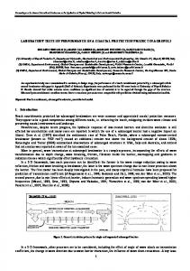
1. INTRODUCTION Severe earthquake damage on bridges, apart from the possible human victims, results in economic losses in the form of significant repair or replacement costs and disruption of traffic and transportation. For these reasons, important bridges are required to suffer only minor, repairable damage and maintain immediate occupancy after an earthquake. The greatest part of existing bridges in Europe and worldwide has been designed before their seismic response had been fully understood and modern codes introduced; consequently they have limited deformation capacity as well as poor hysteretic behaviour and represent a source of risk in earthquake-prone regions. In the absence of codified requirements for existing bridges in Europe, e.g. in Eurocode 8 (EC8) [CEN, 1994], (for the USA see for example the FHWA Seismic Retrofit Manual [Buckle & Friedland, 1995]) and as recent destructive earthquakes cause the revision of seismic maps, there is the need to assess the seismic capacity of existing bridge structures and to study adequate retrofitting techniques. Large-scale tests are a valuable tool in clarifying these aspects. The objective of the research presented in this report was twofold. On one hand, the aim was to develop and implement the non-linear substructuring technique in pseudodynamic testing. This advance in pseudodynamic testing at the ELSA laboratory provides simplified, yet accurate, tools allowing the testing of the complete bridge system using the existing laboratory capacity and reducing considerably the costs of the testing campaign and set-up (two piers instead of six). On the other hand, the aim was the seismic assessment of an existing bridge, shown in Figure B1, that presents characteristics (such as hollow-box cross-section, lapped splices within the potential plastic hinge region, bar cut-off that constitute potential critical zones when tension shift effects develop, low percentage of longitudinal and transverse reinforcement, short overlapping length, inadequate detailing of horizontal reinforcement and lack of appropriate confinement reinforcement) commonly found in existing bridges in Europe and Japan [Hooks et al., 1997].

Figure 1. Talübergang Warth Bridge The project was focused on the Talübergang Warth Bridge, schematically shown in Figure 1. The substructuring method was used with two of the bridge piers, namely A40 and A70, represented by physical models in the laboratory and the rest of the piers, as well as the deck and abutments modelled analytically. Non-linear behaviour

1


was adopted for the substructured piers. Simplified numerical models were calibrated on the results of cyclic tests on large-scale models [Pinto et al., 2001a; Pinto et al., 2001b] and refined analyses [Faria et al., 2001] performed in the first part of the test campaign. For the pier bases and the abutments asynchronous input motion, generated for the bridge site, was considered. Three pseudodynamic tests were performed for input motions with increasing amplitude until failure of the bridge. The geometric characteristics, scaling aspects and material properties of the tested specimens are presented in the next chapter. A description of the pseudodynamic testing method is followed by a discussion of the numerical models for the substructured bridge piers. The pre-test numerical simulation of the PSD test is presented next and the analytical results are compared to the experimental ones allowing to draw conclusions on the implementation of the PSD testing method with substructuring. Three tests were performed and the results in terms of forcedisplacement hysteretic curves, absorbed energy and distribution of dissipated energy in the piers, damage level, drift and ductility demands are discussed for each test. Finally, the seismic performance of the bridge is assessed for the different amplitudes of the earthquake motion. 2. DESIGN OF THE MODELS AND TEST SET-UP On the basis of the results of a pre-test dynamic analysis of the bridge [Gago et al., 1999] it was verified that the piers A40 and A70 would be the mostly damaged. It was then decided to perform the test with these two piers in the lab and the rest of the piers and the deck numerically simulated in the computer. 2.1. Geometric characteristics and material properties The scaling factor, λ = 2.5, was chosen in order to allow for testing within the capacity of the laboratory, to facilitate the construction and to use normal concrete and bar diameters. The relationship for different magnitudes for the prototype and the model is presented in Table 1. The scaled specimens had a rectangular hollow cross-section with external dimensions 2.74x1.02 m. The width of the flange and the web was 0.21 m and 0.17 m respectively. The height of the short pier was 6.5 m (height to length ratio l/D = 2.4) and the height of the tall pier was 14.0 m (height to length ratio l/D = 5.1). The concrete cover was chosen equal to 0.015 m for easiness of construction. The dimensions of the footing, 5.50x2.50x1.20 m, were chosen in terms of the number of anchor rods required to restrain the pier base to the strong floor of the laboratory. The reinforcement of the footing was detailed with 0.23 % reinforcement on the direction of testing (Φ20 mm bars spaced at 12.5 cm), and with 0.15 % reinforcement for shrinkage and temperature on the remaining directions (Φ16 mm bars spaced at 12.5 cm). Spacing at the top of the footing was increased to 25 cm in order to ease pouring of concrete. Twelve DYWIDAG rods placed horizontally across the footing were postensioned in the direction of testing to enhance the strength of the footing and to limit the cracking of concrete. Additional reinforcement at the top of the footing was 2


used to accommodate the compressive forces from the vertical anchor loads. Figure B2 presents various phases of the construction of the specimens, whereas Figure B3 presents the transportation of the model of the short pier inside the laboratory. Table 1. Similitude relationship between the full-scale prototype (P) and the constructed model (M) Quantity Label Relationship Length L LP = λ LM Area A AP = λ 2AM Volume V VP = λ 3VM Mass M M P = λ 3 MM Velocity v vP = vM Acceleration a aP = λ -1aM Force F FP = λ 2FM Time t tP = λ t M Frequency F fP = λ -1fM Strain εP = εM ε Stress σP = σM σ The longitudinal reinforcement of the shaft of the mock-up was detailed to obtain the flexural capacity corresponding to the scaling of the prototype, while representing as best as possible the interaction between concrete and steel reinforcing bars. The last condition requires to keep the steel rebar diameters as close as possible to those of the prototype, while at the same time keeping the spacing, overlapping and anchorage lengths in correspondence to the steel reinforcement diameters used in both the model and the prototype. Splicing of steel reinforcement was kept in the model as close as possible to the prototype. The overlapping lengths were scaled in proportion to the bar diameters. The location and distribution of splicing was maintained throughout the height of the model. Transverse reinforcement was detailed in the model to comply with both the shear capacity and proper spacing in relation to the longitudinal reinforcement; for shear capacity the same percentage of transverse reinforcement was maintained for both the prototype and the model. The longitudinal reinforcement of the short pier A70 consisted of Φ10 deformed bars with volumetric ratio ρs = 0.5 % and the transverse reinforcement consisted of one Φ6 bar at each face of the flange and the web with volumetric ratio ρw = 0.09 %. No stirrups or closed hoops were placed, according to the original design of the pier. Figure C1 presents the reinforcement details of the pier: the starter bars were terminated above the base block and the vertical rebars were spliced just above the base cross-section and within the potential plastic hinge region. The overlapping length was 38Φ, 43Φ and 50Φ for different groups of rebars. The longitudinal reinforcement of the tall pier A40 consisted of Φ12 and Φ16 bars with volumetric ratio ρs = 0.5 %. The transverse reinforcement consisted of one Φ6 bar at each face of the flange and the web with volumetric ratio ρw = 0.09 %. Figure C5 shows the reinforcement details of the pier. The starter bars were terminated above the base block and the following rebars were spliced over a length equal to 38Φ and 47Φ, for different groups of rebars. An other important characteristic of the longitudinal 3


reinforcement, common to piers designed in the same period, is the premature termination of rebars, as a result of pure linear design and of the absence of capacity design. At the height of 3.5 m from the base of the scaled specimen (3.5x2.5 = 8.75 m for the prototype) the longitudinal reinforcement is reduced by almost 50 %: the reduction is 30% for the flanges and 54% for the webs. This fact, together with the tension shift effect, discussed further on, dictated that the moment capacity of that cross-section was reached before the ‘nominal’ flexural resistance of the base crosssection. Thus, the critical cross-section where damage was concentrated was at 3.5 m from the base. Table 2 compares the geometric properties of the tested specimens to the provisions of seismic codes for new bridges in Europe [CEN, 1994; CEN, 1999], the USA [AASHTO, 1995; ATC, 1996; Caltrans, 1999] and New Zealand [SNZ, 1995] for the design values of the material properties. Although all codes forbid the splicing of rebars within the plastic hinge zone, the minimum overlapping length, lo,min, is presented for comparison. All seismic codes require the use of closed hoops or crossties for confinement of concrete and protection of vertical reinforcement against buckling. Both piers fall short of the requirements for seismic detailing. The most noteworthy difference concerns the amount, ρw, and spacing, s, of transverse reinforcement that control the seismic performance of members. Further details on the design of the scaled specimens can be found in [Taucer & Pinto, 2000]. Table 2. Geometrical properties of the specimens and seismic code requirements smin ρs,min (%) ρw,min (%) lo,min Short pier A70 20Φ 0.5 0.09 38Φ-50Φ Tall pier A40 20Φ 0.5 0.09 38Φ-47Φ Europe 6Φ 0.2 0.4 44Φ U.S.A. 6Φ 1.0 0.4 43Φ N. Zealand 6Φ 0.8 0.3 45Φ Concrete C35/45 (characteristic cylinder strength fck = 35 MPa) and steel S500 (characteristic yield strength f0.2k = 500 MPa), as defined in Eurocode 2 (EC2) [CEN, 2000], were used in accordance to the materials specified for the prototype pier. Resulting from tests on cubic specimens, the concrete compression strength was fc = 38.9 MPa for the short pier and fc = 51.6 MPa for the tall pier. The concrete properties are presented in Table 3. Table 3. Concrete mechanical properties for the physical piers (average values) A70 A40 density cubic fc density cubic fc (kg/m3) (MPa) (kg/m3) (MPa) 2363 38.9 2349 51.6 Table 4. Steel mechanical properties for the physical piers (average values) diameter fy ft εmax (mm) (MPa) (MPa) 6 540.2 595.8 0.149 10 543.1 632.6 0.115 12 546.4 660.2 0.065

4


Tests on specimens of reinforcement bars resulted in yield stress fy = 540.2 MPa, fy = 543.1 MPa and fy = 546.4 MPa, ultimate stress ft = 595.8 MPa, ft = 632.6 MPa and ft = 660.2 MPa and maximum strain εmax = 0.149, εmax = 0.115 and εmax = 0.065 for Φ6, Φ10 and Φ12 rebars, respectively. The steel properties are presented in Table 4. 2.2. Instrumentation The instrumentation of the two physical piers was designed with the aim of providing detailed information throughout the height of the specimens and in particular within the regions where significant damage was expected. The instrumentation allows splitting the flexural and shearing deformation. The vertical transducers placed on one web of the pier, at the middle of each flange, throughout the whole height of the pier, were used to measure the rotation of each slice of the pier. The average slice curvature was then computed by dividing the slice rotation by the slice length and the total rotation at the top of each slice was computed as the sum of the slice rotations. The flexural displacement at the top of each slice was calculated on the basis of the computed average slice curvature. The truss of horizontal, vertical and diagonal displacement transducers placed on one face of the pier models was used to calculate the absolute horizontal and vertical displacement of the truss nodes, given the measured relative displacement of each element of the truss. The shear displacement was finally calculated as the difference between the total and flexural displacement. A set of inclinometers was provided along the height of the bridge piers. The rotation measured at the centre of each slice was compared with the value computed using the vertical displacement transducers. Additional inclinometers were placed along the length of one slice to measure the evolution of rotation through the web from one flange to the other. Load cells placed at the piston ends measured the applied forces. Heidenhain optical displacement transducers attached to an independent reference frame measured the pier top displacement. Each piston was equipped with a Temposonics displacement transducer. One displacement transducer was provided for every pier in the direction parallel to the flange to measure the eventual lateral displacement of the specimen. Details on the instrumentation and complete drawings can be found in the previous reports on the cyclic tests on the two pier models [Pinto et al., 2001a; Pinto et al., 2001b]. Figure B4 shows the two physical piers in the lab before testing. 2.3. Application of the vertical load The vertical load on the piers was applied by means of 8 internal post-tensioned vertical DYWIDAG rods. One end of each rod was anchored in the pier base block. The other end of the vertical rebar was attached to a hydraulic actuator applying a tensile force on the rebar. The total vertical load on the pier was kept constant throughout the test by a self-compensating system. Two different techniques were used for the control of the vertical load applied through these pistons. For the tall pier A40, the eight pistons were grouped in four couples and for each couple, one of the pistons 5


was provided with a servovalve that served oil for both the pistons and was controlled to apply a constant force for the piston couple. For the short pier A70, all the eight pistons were just connected to an oil accumulator, which kept an almost constant pressure even for the case of small vertical displacements at the top of the pier. This passive system allowed being accurate enough for the force control of the short pier. The values of axial load applied on each one of the physical piers were estimated according to a procedure explained in detail in a following paragraph. The system for the application of the vertical and horizontal loads for the two physical piers is shown in Figures B5 and B6. 3. THE PSEUDODYNAMIC TESTING METHOD WITH SUBSTRUCTURING 3.1. Pseudodynamic testing of large-scale structures A PSD test [Shing & Mahin, 1985; Nakashima et al., 1992; Donéa et al., 1996] is one, which, although carried out quasi-statically, uses on-line computer calculation and control together with experimental measurement of the actual properties of the structure to provide a realistic simulation of the dynamic response. For simulating the earthquake response of a structure, a record of a real or artificially generated earthquake ground acceleration history is given as input data to the computer running the PSD algorithm. The horizontal displacements of the controlled degrees of freedom (DOFs), where the mass of the structure can be considered to be concentrated, are calculated for a small time step using a suitable time-integration algorithm. These displacements are then applied to the tested structure by servo-controlled hydraulic actuators fixed to the reaction wall. Load cells on the actuators measure the forces necessary to achieve the required displacements and these structural restoring forces are returned to the computer for use in the next time step calculation. Because the inertia forces are modelled, there is no need to perform the test on the real time-scale, thus allowing very large models of structures to be tested with only a relatively modest hydraulic power requirement. It is generally not feasible to test structures as large as bridges or offshore platforms. However, earthquake loading often generates severe damage only in parts of the structure. It is expected that the rest of the structure could be modelled via finite elements or other numerical techniques. Therefore it is useful to think of combining PSD testing of only a part of the structure, the tested structure, together with an adequate time-integration of the equations of motion for the model of the rest of the structure, the modelled structure (e.g. the deck). To this purpose a substructuring technique is proposed [Dermitzakis & Mahin, 1985], considering either synchronous or asynchronous base motion. 3.2. The α-Operator Splitting scheme Consider the following system of semi-discrete differential equations

6


Ma + Cv + r(d) = f

(1)

which describe the motion of a structure, where a, v and d represent the acceleration, velocity and displacement vectors, r and f the structural internal and external force vectors, M and C the mass and damping matrices. In the case of synchronous seismic loading, a, v and d represent the motion of the structure in a reference frame which is relative to the uniform ground motion. The seismic action is taken into account by means of an inertial contribution to the external force vector f = -MIbasea

(2)

where basea is the intensity of the base acceleration and I is a vector that accounts for the direction of earthquake loading at the level of each DOF. To solve the system of equations given by Equation (1), a numerical step-by-step integration technique is adopted: in this work it is the so-called α method implemented by means of an Operator Splitting (OS) technique. This scheme is unconditionally stable and does not require iterations. According to the α method [Hilber et al., 1977], the displacement and velocity vectors at step (n + 1) can be written in terms of both the acceleration vector and the previous step values ~ dn+1 = d n+1 + ∆t2 β an+1

(3)

~ n+1 d = dn + ∆t vn + 0.5 ∆t2 (1-2 β) an

(4)

vn+1 = ~ v n+1 + ∆t γ an+1

(5)

~ v n+1 = vn + ∆t (1- γ)an

(6)

β = (1 - α)2 / 4

(7)

γ = (1-2α) / 2

(8)

with

for –⅓ ≤ α ≤ 0 and then introduced into the following time discrete system of equilibrium equations M an+1 + (1 + α) C vn+1 – α C vn + (1 + α) rn+1 – α rn = (1 + α) fn+1 – α fn 7

(9)


This scheme is implicit since dn+1 depends on an+1 related to rn+1, which is a function of dn+1, and then it implies an iterative procedure. It is however possible to implement the method without iterating by using an Operator Splitting method [Combescure & Pegon, 1997], based on the following approximation of the restoring force rn+1 ~ ~ rn+1(dn+1) ≈ KI d n+1 + ( ~r n+1( d n+1) – KI d n+1)

(10)

where KI is a stiffness matrix, generally chosen as close as possible to the elastic one, KE, and in any case, for stability reasons, higher or equal to the current tangent stiffness, KT(d), of the structure. Note that the digital PSD experimental set-up clearly offers all what is needed for an accurate measurement of the elastic characteristics of the structure to be tested or of its current stiffness at the beginning of any test. All useful quantities being known at time tn, the step-wise operations for reaching the time tn+1 = tn + ∆t are ~ (i) Compute (prediction phase) d n+1 and ~ v n+1. ~ (ii) Apply (control phase) the displacement d n+1 to the tested and the numerical structure in order to get (measuring phase) the restoring force ~r n+1.

(iii) Solve for an+1 the system of linear equations ˆ an+1 = fˆ n+1+ α M

(11)

ˆ and the pseudo-force vector fˆ n+1+ α are given by where the pseudo-mass matrix M ˆ = M + γ ∆t (1 + α) C + β ∆t2 (1 + α) KI M

(12)

and fˆ n+1+ α = (1 + α) fn+1 - α fn + α ~r n - (1 + α) ~r n+1 + a C ~ v n - (1 + α) C ~ v n+1 +

α (γ ∆t C + β ∆t2 KI ) an (iv) Compute (correction phase) dn+1 and vn+1.

8

(13)


ˆ , which usually does not Note that the computation, and possibly the factorisation of M depend on the time, may be performed during the initialisation phase of the algorithm, before entering the time stepping loop. Note also that the verification of the α-shifted system of equilibrium equations, Equation (11), makes the pseudo-force vector fˆ n+1+α dependent on α. Furthermore, Dirichlet boundary conditions, such as the base acceleration and the connection between tested structure and modelled structure, must also be dealt in the α–shifted system, in the same way as the inertial external force in Equation (13). 3.3. The substructuring technique

It is generally not feasible to test structures as large as bridges or offshore platforms. However, earthquake loading often generates severe damage only in parts of the structure and the rest of the structure could be modelled via finite elements. Therefore, it is useful to combine PSD testing of only a part of the structure, the tested substructure, together with an adequate time-integration of the equations of motion for the model of the rest of the structure, the modelled substructure. To this purpose a substructuring technique is proposed, considering either synchronous or asynchronous base motion. The modelled substructure must be approximated by an adequate numerical model and the time-integration scheme must be applied to its spatially discrete equations of motion. The strategy adopted in the past [Pegon & Pinto, 2000] was to run two processes in parallel. The one responsible for the PSD algorithm applied to the tested structure, running in the master PSD computer, a PC, and the other, responsible for the modelled structure, running in a remote workstation. The communication between these two processes used standard network capabilities. In the meantime, the experimental side was updated to run the continuous PSD method, where the motion of the structure is controlled every msec (10-3 sec). 3.4. Substructuring in the case of asynchronous motion

For the PSD tests with asynchronous input motion [Pegon, 1996a], special attention has been devoted to the mathematical and implementation aspects, which is the object of this section. In fact, the PSD testing with substructuring for asynchronous motion is not only a trivial extension of the case with synchronous motion. The main difficulty at the mathematical level comes out from the fact that the structure in the laboratory can only be tested in a reference frame relative to the earthquake motion because its base is always fixed to the floor. Then, in order to realize a meaningful test on a structure (tested and modelled substructures) undergoing an asynchronous motion, only physically unconnected parts of the tested structure can be submitted to different base accelerations. This condition is easily verified for bridges: the tested substructure consists of a set of different piers, which do not interact one with the others, apart through the modelled deck.

9


Equation (1) may describe a relative or an absolute motion. The description with a relative motion is the most widely used in earthquake engineering. The base of the structure of interest is considered to be subjected to a uniform base acceleration field base a. The basic principle of the dynamics is expressed in a reference frame, which follows this ground motion. The motion of the structure is originated by the inertial forces considered as being part of the external force vector f, see Equation (2). The relative motion description is quite natural since it expresses directly the contribution of the structure response to the overall motion. The description with an absolute motion is scarcely used, only when the other approach is impossible. This is the case of an asynchronous ground motion where the base acceleration field changes spatially from point to point. The motion of the structure is now originated by the motion of some of its internal points. In consequence, provision should be made while performing the discretisation of the structure not to eliminate the ground connecting DOFs and to subject them to the convenient base acceleration basea (Dirichlet boundary condition). Clearly, in the case of synchronous motion, both descriptions lead to the same results in terms of intensive variables (internal stress state for instance). 3.5. The continuous pseudodynamic testing with non-linear substructuring

In the conventional PSD test procedure, the actuator motion (S-ramp phase) is stopped when the test specimen reaches the target displacement (hold period), so that the reaction force can be measured and the next target displacement computed. On the contrary, in continuous PSD testing, the servo-controller moves the actuator continuously. The continuous PSD testing avoids the load relaxation problem and consequently improves the quality of the results. It allows a considerable reduction of the test duration. The continuous PSD method is implemented by means of a synchronous process (in electronics terms: communication to the outside is clock-governed) with short control period and small time step. This introduces some difficulties for the implementation of the substructuring technique. First, if the numerical part is complex, the analytical process is unable to perform even an elastic computation during a control period of the experimental process. In addition, it is not evident that using the same explicit scheme for both the experimental and analytical processes would allow to obtain stable results. Finally, the exchange of information between the two processes should not add a too large overhead. The experimental process of the continuous PSD method is synchronous and then unable to wait for information coming from the analytical process. Thus, a parallel inter-field procedure should be used. For the simple inter-field procedure, see Figure 2a, the analytical part is advanced with a large time step, ∆t, using, possibly, at each new step the acceleration, velocity and displacement of the connection points obtained through the experimental process at the end of the previous large step. On the contrary, the experimental part uses at each subcycle, δt, as an additional external force, what

10


was generated in the analytical part at the end of the previous large time step. The main drawback of this approach is that the force coming from the numerical part is not well synchronized with the external loading of the physical model. This delay introduces damping when the experimental and analytical processes are strongly coupled, i.e. have similar mass. On the contrary, for the case of the numerical part having bigger mass than the experimental (representative of bridges with experimental piers and numerical deck), slowly increasing oscillations, associated with higher frequencies, were observed. Introducing subcycling in the experimental part does not significantly improve the results [Pegon & Magonette, 1999]. An improved scheme is introduced, in which the modelled structure is integrated with a time step 2∆T, see Figure 2b. This allows to know the kinematics of the numerical structure one large time step in advance with respect to the tested part. Then, an approximation of the additional force r n+1 at time tn+1 is known before starting the subcycling between tn and tn+1. It is thus possible to drive the experimental structure with more updated information than with the basic scheme. The force r n+m/M that is used in the experimental process at each subcycle level can be simply r n+m/M = r n+1; m = 1…M

(14)

However, since r n is also known, it is possible to use both quantities to improve the time-integration accuracy. The additional force that enters the algorithm for the experimental substructure can be interpolated as r n+m/M = r n+1 – (1 – m/M) ( r n+1 – r n)

(15)

Using this scheme, improved results are obtained, compared to those obtained with the simple scheme. However, the method is conditionally stable, depending on the distribution of mass on the connecting DOFs and on the time step. The error is reduced when reducing the time step, but convergence is slow. The number of subcycles does not seem to significantly improve the results [Pegon & Magonette, 2002]. Considering the time-integration schemes for non-linear substructuring, it was found that explicit schemes can be used for the analytical part only when a small number of DOFs is involved, whereas implicit schemes depend strongly on the local nature of the problem and could result in significant local deviations from the medium time step duration [Pegon & Magonette, 2002].

11


Figure 2. Parallel procedures: simple inter-field procedure (a), improved inter-field procedure (b) and intra-field procedure

12


3.6. Implementation for the Talübergang Warth Bridge tests

The inter-field procedures are not yet robust enough to be applied in large-scale testing of bridge structures. The problem was solved using an intra-field procedure (a unique main process delegating all the piers tasks to other processes) rather than an inter-field procedure (two or more processes running in parallel), see Figure 2c. The experimental and numerical parts are advanced in time (subcycling is introduced in both) and exchange information at the end of the time step, through the Modelling Master workstation.

Figure 3. PSD test with substructuring for the Talübergang Warth Bridge The implementation of the substructuring technique for the Talübergang Warth Bridge PSD tests is schematically presented in Figure 3, which includes three main workstation groups, namely: the Experimental Master, the Physical models and the Numerical models. The Numerical models group includes the Modelling Master workstation (holding the linear model of the deck and the lateral DOFs of the piers), which performs the time-integration of the motion of the whole bridge, using the α-OS scheme. Each pier, either modelled or tested, is condensed on two DOFs, namely the base and the top displacement. Obviously, it is the difference of the displacement of these two DOFs that is transmitted as target to the controller of the pier. The force, which is measured and transferred back to the numerical process, is then associated to the two DOFs with the sign. As soon as the predicted displacement, d , see Equation (3), is computed, the displacements to impose to the analytical piers are sent to two other computers (Modelling Slaves) holding the non-linear model of the piers and using an iterative

13


process to equilibrate the internal nodes of the discrete model. The displacements to impose to the experimental piers are sent to the Experimental Master, which in turns generates the appropriate elongated ramp curve (S-shaped displacement-ramp and elongated sustain-level plateau) to be reached by two controllers, each of them responsible for one experimental pier. The communication is implemented in such a way that if the numerical piers require a large number of iterations at the interior of one step, the controllers of the physical piers can wait (further small time steps are performed) for the input of the next time step. Actually, the time required to perform the numerical integration for the substructured piers was always inferior to that value during the pre-test calculations. When the analytical piers are equilibrated and the experimental piers attain the target displacement, the force levels reached at the ends of each pier are transmitted back to the Modelling Master in order to compute the next displacement. The communication between the workstations is done via the laboratory local network. 4. NUMERICAL MODELS FOR THE SUBSTRUCTURED PIERS

In order to reduce the computation demand for the PSD tests and to increase the robustness of the numerical models and procedures, a simple, yet accurate numerical model should be used for the substructured piers. The Fibre/Timoshenko beam model [Guedes et al., 1994] was chosen. Taking into account the symmetry of the geometry and the loading, a two-dimensional (2D) beam element was used. Different simplified configurations at the cross-section level have been examined, as explained in detail in the following. Non-linear behaviour was assumed for the concrete and a modified Menegotto-Pinto or elastic-perfectly plastic behaviour for the reinforcement steel. Table 5 presents the material properties used in the numerical model. Since no closed stirrups or crossties are present, no confinement effect was considered for the concrete fibres.

Ec (GPa) 33.5 Es (GPa) 200

Table 5. Material properties ν fc (MPa) ft (MPa) εo 0.2 43 3 0.00257 ν 0.3

fy (MPa) fu (MPa) 545 611

εy 0.005

4.1. The Fibre/Timoshenko Beam element in Cast3m

Numerical pre-test analyses have been performed using a Fibre/Timoshenko Beam element implemented in the finite element code Cast3m [Millard, 1993]. A two-level approach is adopted for this model: the first is the description of the section (fibre elements) and the second is the description of the Timoshenko beam. The evaluation of the stress resultant for each beam element proceeds as follows

14


(i) Evaluation of the generalized strain Ε at the integration point of each beam element, from the nodal generalized displacement (U1, Θ1, U2, Θ2). (ii) Use of the beam model in order to evaluate the strain tensor ε and in particular its normal component εx, at the level of each fibre, located at the Gauss integration points of the elements describing the section. (iii) Use of the constitutive relationship in order to evaluate the stress tensor σ at the level of each fibre, in particular its normal component σx. (iv) Integration over the section of the relevant stress components in order to compute the generalized stress F for the section. (v) Computation of the stress resultant (F1, M1, F2, M2) for the beam element. 4.2. Alternative models for the cross-section

Different configurations have been examined for the discretisation of the cross-section of the piers. With the aim of reducing the computation effort an attempt was made to simplify the numerical models, taking into consideration the symmetry of the crosssection and the loading. The results of each alternative configuration were compared and the adopted numerical model was calibrated on the basis of the cyclic tests performed on scaled models (1:2.5) of the tall and short piers (A40 and A70 respectively).

Figure 4. Dimensions of the scaled (1:2.5) pier cross-section

15


4.2.1. The equivalent I cross-section

The scaled bridge piers have a hollow box cross-section schematically shown in Figure 4. The dashed line shows the centre line of the vertical reinforcement bars. The corresponding fibre model for the cross-section is presented in Figure 5a. The elements shown in blue correspond to the (unconfined) concrete, whereas those shown in red correspond to the vertical reinforcement steel. Each element used to model the reinforcement has eight integration points and an area equal to the area of the reinforcement of each face of the cross-section. This configuration was initially chosen in order to be close to the geometry of the specimens. Keeping in mind that the displacement would be imposed parallel to the wider direction of the cross-section, the discretisation adopted for the steel was considered adequate for the flanges, but not for the web. The vertical rebars in the specimen were uniformly distributed along the two faces of the web and were expected to be under tension gradually as the neutral axis moves along the web: this cannot be accurately modelled with the initial configuration and could cause problems during the iterations for the PSD testing with substructuring. The mesh for the cross-section was therefore refined in order to avoid such numerical problems.

(c) (a)

(d)

(b)

Figure 5. Discretisation of alternative models for the cross-section Since the cross-section was symmetric and the loading was applied along an axis of symmetry, an alternative model at the cross-section level was examined, shown in Figure 5b. An equivalent I cross-section was considered with a web width equal to the total width of the two webs of the original cross-section. Rectangular elements with four integration points each, better distributed along the web were used for the web reinforcement. This configuration enabled a more realistic representation of the actual distribution of vertical reinforcement along the web of the pier model. With almost the same computation effort as for the box cross-section, but with more elements along the direction of the imposed displacement, smoother curves of moment-curvature and force displacement were obtained. This would demand less computation time during the PSD tests.

16


4.2.2. New elements implemented in Cast3m

In an attempt to further simplify the model, a new element was implemented for the reinforcement steel. The element used originally, ‘QUAS’, is a linear quadrilateral element with four nodes. In order to reduce at minimum the integration points, the ‘POJS’ element with one integration point was implemented. The geometrical support is a point, thus there is only one integration point instead of four. This enabled the use of elements better distributed to model the vertical rebars. The corresponding model of the cross-section is shown in Figure 5c. The computed curves for moment-curvature and force-displacement were consistent with those obtained using the previous models. In an attempt to further simplify the model and consequently meliorate the speed of computation of the substructured models during the PSD tests, a new element was implemented for the concrete fibres. The new ‘SEGS’ elements have only two integration points, since their geometrical support is a segment. The width of each element and the coefficient multiplying the shear stress are characteristic properties of the element. The corresponding model at the cross-section level is shown in Figure 5d. 4.3. Alternative models for the beam element

The original Timoshenko beam model was used to perform analysis in three dimensions (3D), and thus six DOFs were considered for each node of the beam elements. The calculated reactions are then Rx, Ry, Rz, (forces along the three axes) and Mx, My, Mz (moments by the three axes). Considering the symmetry of the geometry and the loading, only 3 DOFs were significant in the present case for the piers; namely displacements along the vertical and longitudinal axes and rotation by the transverse axis. A 2D beam element was used considering the cross-section shown in Figure 5: the results were in agreement with the previous ones. Table 6. Characteristics for different models crossconcrete steel beam Fultimate section elements elements model (kN) A20 hollow box section section 3D 1123 A20I I section section 3D 1244 A20I1 I section point 3D 1166 A20I_2D I section point 2D 1176 A20s I segment point 2D 1131

uultimate (m) 0.15 0.20 0.15 0.17 0.18

The results of all alternative models at the cross-section level are presented in Figures A1 and A2 for the pier A20. Table 6 recapitulates the type of cross-section and elements used for every alternative model. Note that the results presented in Figures A2 and A2, as well as in Table 6, come from the numerical model in which the modified Menegotto-Pinto model for steel was used. The values of force and moment at the characteristic points of yield and ultimate capacity were similar in all cases. The values of displacement and curvature, though, were different. It should be noted that an increase in the number of elements used for the web vertical reinforcement resulted in decrease in the value of ultimate displacement and curvature. The decrease was even 17


bigger when each rebar was considered separately (A20I1, A20I-2D and A20s) instead of considering groups of rebars (A20 and A20I). The geometry of the cross-section (hollow box or I-shaped) did not seem to have a similar effect. 4.4. Calibration on the basis of cyclic tests

Before the PSD tests, two scaled piers were tested under cyclic loading until failure [Pinto et al., 2001a; Pinto et al., 2001b]. The main objective of the cyclic tests was the calibration of the numerical models for the substructured piers. The results of numerical simulations using a damage model [Faria et al., 2001] were also compared to the experimental values. The fibre model is adequate for the case of the short pier A70. The failure mode was flexure-dominated and the deformation demand was concentrated within a thin slice at the base of the pier. The results of the numerical analyses are compared to the experimental values in Figure A15. The numerical pier A20 was expected to have a similar failure mode. Concerning the tall pier A40, the fibre model resulted in larger resistance, whereas the damage model gave values similar to the experimental ones. It is reminded that the failure in the tall pier did not occur at the base, but at the cross-section at height h = 3.5 m, where a significant reduction of the reinforcement takes place. The same failure mode and overall behaviour was expected also for the numerical piers A30, A50 and A60, that presented curtailment of vertical reinforcement. The fibre model was unable to accurately represent the strut effect due to shear in the lower part of the specimen.

Figure 6. Equilibrium of forces in diagonally cracked element Considering the equilibrium of a diagonally cracked element with shear reinforcement, see Figure 6, we can define the following forces acting on a cross-section: Fc is the compressive force on concrete, Ft is the tension force on longitudinal steel and in addition we can consider the uniformly distributed inclined forces of the transverse steel (tension forces) and the concrete strut (compression forces). From equilibrium of these forces and the external axial load, N, and bending moment, M, we obtain Fc = M / z – ys1 V (cotθ – cotα) / z ≈ M / z – 0.5V (cotθ – cotα)

18

(16)


and Ft = N + M / z + ys1 V (cotθ – cotα) / z ≈ N + M / z + 0.5 V (cotθ – cotα) (17) where θ is the inclination of the cracks with respect to the element axis (it can be considered approximately θ = 45°), α is the angle of the transverse reinforcement (in this case, α = 90°), ys1 is the distance between the reinforcement centreline and the cross-section centroid and z is the internal lever arm of the cross-section. The last term in the above expressions is due to the diagonal shear cracking and is additive to the forces due to pure bending. It is evident that after the development of diagonal cracks the tension force acting on the longitudinal reinforcement is greater than that required to resist the bending moment. This phenomenon is termed tension shift [Paulay & Priestley, 1992; Park & Paulay, 1975]. In EC2 [CEN, 2000] it is taken into consideration by shifting the moment curve towards the unfavourable direction by a distance calculated by the expression al = z (cotθ – cotα) / 2

(18)

which is in agreement with the previous theoretical expressions. Since shear is not fully taken into consideration in the fibre/beam model, an alternative configuration was studied with a moment proportional to the top force applied at the height where failure occurred. The results of this model were closer to the experimental values, as seen in Figure A4. As during the PSD test the input for the substructured piers would be the displacement at the top, this solution was complicated. For this reason, it was decided to reduce the amount of longitudinal steel in the flange above the critical cross-section. The reduction was such to obtain the correct failure location and resistance and to approximate as much as possible the cyclic behaviour and energy dissipation capacity. The results of the damage model were used as the target resistance. The amount of dissipated energy was calculated for all piers and the two different modelling solutions and is presented in Table 7, along with the experimental values for the short and the tall piers. The modified fibre model dissipated a larger amount of energy (closer to the experimental value for piers A40 and A70), whereas the damage model resulted in less energy dissipation in all cases. Table 7. Absorbed energy (kNm) A20 A30 A40 A50 A60 A70 Damage model 27.7 126 227 97 79 296 Fibre model 34.4 223 280 162 145 332 274 321 Experimental1 1 previous cyclic tests [Pinto et al., 2000a; Pinto et al., 2000b] For the above reasons it was decided to use a fibre model with reduced area of longitudinal reinforcement in the flange above the critical cross-section for the substructured piers A30, A50 and A60. The corresponding force-displacement and

19


absorbed energy curves are presented in Figures A5 to A16. The characteristic values of force and displacement at cracking, ‘total’ yielding and failure, as resulting from the adopted models are presented in Table 8 for all the piers. Displacement ductility is defined as the maximum attained displacement divided by the displacement at ‘total’ yielding. For piers with elongated cross-sections and distributed reinforcement, where progressive yielding of the longitudinal reinforcement and fluctuation of the neutral axis occur after first yielding and until the stabilization of strength (‘total’ yielding), a trilinear diagram (with two characteristic points: first yielding/cracking initiation and ‘total’ yielding) is a good approximation of the experimental data. For the above reasons, the initial stiffness is defined by a line from the origin to the experimental curve at 75% of the maximum strength. The stiffness of the second branch is an approximation of the experimental curve that satisfies the equal energy criterion and zero stiffness is assumed after ‘total’ yielding. Total yielding can be significantly different than first yielding, corresponding to yielding of the first steel fibre. Quite often, ‘nominal’ yielding is used. Nominal yielding is defined, considering an elastic-perfectly plastic approximation of the monotonic curve of the pier, at the intersection of the horizontal line at the maximum strength, Fmax, and the line from the origin passing through the curve at F = 0.75Fmax [Park, 1989]. All relevant values are presented in Table 8. Table 8. Values of force and displacement for the bridge piers A20 A30 A40 A50 A60 A70 Fcrack (kN) 541.7 438.6 460.2 366.0 415.1 777.0 ucrack (m) 0.010 0.018 0.013 0.009 0.006 0.003 810.0 604.8 776.8 570.4 675.9 986.5 Fyield (kN) 0.030 0.045 0.064 0.049 0.038 0.009 uyield-first (m) uyield-nominal (m) 0.050 0.042 0.081 0.056 0.058 0.010 0.099 0.115 0.100 0.102 0.083 0.025 uyield-total (m) 1107.0 721.5 784.4 669.6 831.4 1252 Fultimate (kN) 0.187 0.372 0.230 0.326 0.179 0.100 uultimate (m) 1.9 3.2 2.3 3.2 2.2 4.0 µu Finally, Table 9 presents the reinforcement areas adopted for the substructured piers, after the modifications in order to take into consideration the tension shift effect. Table 9. Vertical steel areas (cm2) for the substructured piers A20 A30 A50 A60 A-A l1 = 2.76 m l1 = 3.52 m l1 = 1.60 m l1 = 1.48m flange 1.7608 2.316 2.444 1.652 web 9.4458 6.286 6.027 7.7812 B-B l2 = 7.04 m l2 = 7.08 m l2 = 7.24 m l2 = 2.68 m flange 1.5436 0.4624 0.5499 0.46308 web 6.0466 3.2200 3.087 4.5668 C-C l3 = 2.12 m l3 = 4.96 m l3 = 5.56 m l3 = 7.84 m flange 1.2388 1.0200 1.1016 1.1016 web 2.1686 1.4000 2.7258 2.7258

20


5. PRE-TEST NUMERICAL SIMULATION OF THE PSD TESTS

Pre-test dynamic analysis was performed with the aim of predicting the earthquake response of the bridge. The results of the dynamic analysis were compared to the results of the numerical simulation of the PSD test in order to assess the ability of the latter to represent a real earthquake test. In order to better represent the PSD test, the numerical model of the bridge was simplified in comparison to the real structure.

Figure 7. Dimensions of the scaled deck cross-section 5.1. Description of the model

The deck was modelled using a fibre/Timoshenko beam element [Guedes et al., 1994] with a cross-section schematically shown in Figure 7. The height of the scaled model was 2.00 m and the width of the top and bottom flanges was 5.00 m and 2.48 m, respectively. The area of the cross-section is A = 1.57 m2, while the moment of inertia is Iyy = 3.35 m4 and Ixx = 3.18 m4 by the vertical and horizontal axes, respectively, and the rotational moment of inertia is J = 2.72 m4, see Table 10. The deck was considered to remain elastic, in accordance with the requirements of modern codes for new bridges, e.g. [CEN, 1994; Caltrans, 1999], and assumptions commonly used in the design and retrofit of bridges [Priestley et al., 1996]. For the deck all 6 DOF by node have been kept in order to better describe the coupling between translation, bending and torsion of the deck. Nine elements were used along each span. Table 10. Geometric properties of the deck cross-section Iyy (m4) Ixx (m4) J (m4) A (m2) 1.5 3.35 3.18 2.72

21


The model adopted for the piers was the one with 3 DOFs by node described in the previous section. Each pier was divided in an adequate number of elements along its height; more elements were used in the region where damage was expected and less elements near the top of the pier, where the behaviour was expected to be elastic. The number and distribution of the elements was chosen such to obtain reliable results with the minimum computation demand. The foundation blocks of the piers were considered to remain elastic and to be fixed along all 3 DOFs. This was the case for the physical models of piers A40 and A70 in the lab, but may not be the case for the real structure due to soil-structure interaction. As stated before, all 6 DOFs per node were considered for the deck whereas only 3 DOFs per node were considered for the piers. An adequate connection between the corresponding DOFs of the deck and the top of the piers was established in the model. Only the vertical and horizontal forces in the direction of testing (orthogonal to the bridge axis) were transmitted between the piers and the deck. The abutments constrained the displacement in all three axes and the rotation by the bridge axis. During the PSD test only the DOF at the top of the piers (where the mass of the pier is considered to be lumped) was controlled, therefore a concentrated external load was applied on the top of the piers to take into consideration the vertical static forces transmitted by the deck and the pier self-weight. During the test constant vertical forces were applied on the physical models of the two piers. The distributed mass of the piers was taken into consideration when calculating the vertical force but had no contribution to the lateral loading. The vertical loading can be considered comprising two parts. The first part results from the mass of the deck. This is the reaction force at the top of the pier computed by an elastic analysis. The second part results from self-weight of the piers. Following the similitude relations in Table 1, the stress at the base cross-section of the prototype and the model should be equal. This means that the stress applied on the model should be σ = MP g / AP = 2.5 MM g / AM, where M denotes the mass of the pier and A the area of the base cross-section. However, the mass of the pier, corresponding to a stress equal to MM g / AM, is already present. Then, the vertical force on the physical piers is calculated based on the mass of the model multiplied by 2.5 – 1 = 1.5. The general non-linear procedures in Cast3m [Millard, 1993] were modified and adapted to this particular kind of analysis. It is noted that Cast3m is a general-purpose program that can perform mechanical, liquid, thermal, radiation, magnetodynamics etc analysis. The procedures used for the pre-test numerical simulation and also during the PSD tests were specialised to mechanical analysis using only plastic-like material and consequently simplified. In this way a number of insignificant checks was avoided and a smaller computation time was achieved.

22


5.2. Damping matrix

The damping matrix was formulated by considering only the contribution of the deck (it is expected that the piers will have small hysteretic damping, at least for the smallamplitude earthquakes) and assuming a truncated modal damping [Pegon, 1996] in order to avoid problems related to rigid body motion in the case of asynchronous loading. This expression of damping is based on the commonly used Rayleigh damping, e.g. [Clough & Penzien, 1993], that consists of two parts, one proportional to the mass of the structure and the other proportional to the stiffness C = αo M + α1 K

(19)

In the modal space Rayleigh damping takes the form

ξiR = ξiRM + ξiRK =

α o α1ωi + 2ωi 2

(20)

For the truncated modal damping the mass-proportional damping is distributed to the n first modes and then added to the stiffness-proportional damping. In matrix form it writes C= ∑ in=1 C iM + α K

(21)

The mass-proportional damping matrix is C iM = M ψ dM ψT M

(22)

where ψ contains the eigenvectors and the terms of the diagonal matrix dM are

d iM = 2 ωi ξiRM / mi; i = 1…n

(23)

The proportionality coefficient, α, of Equation (21) is calculated by assigning the Rayleigh damping value of the n+1 mode, ξ Rn +1 , to the stiffness-proportional damping α = 2 ξ Rn +1 / ωn+1 Then, the modal mass-proportional damping can be written as

23

(24)


ξ iM = ξ iR - ξ Rn +1

ωi ; i = 1…n ω n +1

(25)

For the present case the first seven (n = 7) modes were taken into account. 5.3. Modal analysis

The eigenfrequencies of the bridge structure were identified by using the numerical model. Experimental measurement of the natural frequencies of the bridge structure has been performed [Flesch et al., 1999; Flesch et al., 2000] by dynamic in-situ tests and is reported in Table 11 along with the numerical ones. Figure A3 presents the first natural eigenmodes (horizontal and vertical) of the structure as calculated using the numerical model. It is reminded that the scaling factor, λ = 2.5, applies to the eigenfrequencies: the values for the model are obtained from the values for the prototype multiplied by the scaling factor. Since the analytical values were similar to the experimental ones, the numerical model for the bridge seems capable of representing the modal properties of the bridge structure. Table 11. Eigenfrequencies of Talübergang Warth Bridge (1[Flesch et al., 1999], 2 [Flesch et al., 2000]) 1 analytical (Hz) mode experimental (Hz) experimental2 (Hz) 1 0.796 0.80 0.9988 2 1.095 1.10 1.2093 3 1.584 1.62 1.6978 4 2.194 2.23 2.2861 5 2.907 2.98 2.7052 6 3.709 3.77 3.1592 7 4.863 8 5.828 5.4. Input motion

Considering the spatial variability of the ground motion, its main sources are the finiteness of the seismic source, the geological and geometrical heterogeneities of the foundation soil and the wave-passage effects. According to EC8 [CEN, 1994], the spatial variability of the input motion at the supports of bridges must be taken into consideration for long bridges in the presence of geological discontinuities or marked topographical features. Similar guidelines are provided by the Caltrans Seismic Design Criteria [Caltrans, 1999]. The Japanese seismic code [JSCE, 1996] requires the consideration of epicentral characteristics and amplification of the surface layer in defining the design input motion for the design earthquake with a rare probability of occurrence. The New Zealand Standards [SNZ, 1995] recognize the need to increase the seismic loading due to site effects, but does not directly take into consideration asynchronous motion of multi-support structures. Alternatively, it is proposed to provide movement joints [Priestley et al., 1996].

24


It has been proved [Monti et al., 1996] that designing for rigid motion provides a global upper bound of the response. Experimental results of an irregular bridge tested under asynchronous earthquake input [Calvi & Pinto, 1996; Pinto, 1996] verify these findings. On the other hand, a theoretical study [Der Kiureghian & Neuenhofer, 1992] considering asynchronous motion due to wave- passage and incoherence effects as well as local soil conditions, proved that in certain cases, e.g. stiff structures, the differential support motion may result in larger internal forces An analytical study of a regular bridge subjected to non-stationary multi-support random excitation [Perotti, 1990] suggests that the internal forces are in general reduced for both the deck and the piers, but in certain cases an increase was observed. Dynamic analysis of a regular bridge structure considering local soil amplification [Zembaty & Rutenberg, 1998] suggests significant amplification of shear forces and displacements for substantial soil amplification. Dynamic analysis of an existing regular bridge [Kahan et al., 1996] showed that for small variability of the ground motion the shear forces are decreased and the displacements increased, compared to synchronous input for both longitudinal and transverse motion. Nevertheless, the limited number of studies does not permit the generalization of these findings without further experimental and numerical investigation, particularly for the case of irregular bridges. The input motion for the Talübergang Warth Bridge tests was defined by an artificial accelerogram provided by ICTP [Panza et al., 2001]. Based on the local soil conditions, different focal depths, distance and source mechanisms, the displacement, velocity and acceleration time histories were calculated. Different accelerograms at the bases of the piers and the abutments were also provided for the case of asynchronous motion. Some treatment of these accelerograms was performed in order to have a uniform distribution of the time step, null final displacement and velocity, null average velocity and correct scaling, according to Table 1. The input accelerograms are presented in Figure A17 for the Nominal Earthquake (1.0xNE), corresponding to the Ultimate Limit State. Three earthquake motions were used as input, corresponding to the given accelerograms multiplied by 0.4 (0.4xNE, hypothetically corresponding to the Serviceability Limit State), 1.0 (1.0xNE) and 2.0 (2.0xNE, corresponding to significant non-linear response of the structure). Loading in the transverse bridge direction alone was considered. 5.5. Numerical simulation of the PSD tests

The PSD tests were numerically simulated in order to validate their representativeness of an earthquake test. The same model and assumptions considered for the dynamic analysis were used for the numerical simulation of the PSD tests with the difference that only the horizontal forces in the direction of loading were transmitted between the deck and the piers, since the substructuring method would be applied. In addition, both an implicit, iterative and the α-OS explicit schemes [Combescure & Pegon, 1997] were used for the time-integration of the equation of motion. The results of the numerical simulation of the PSD test were compared to the results of the dynamic analysis. The same input motion used for the dynamic analysis was used for the numerical simulation of the PSD tests for both the explicit and implicit iteration schemes.

25


The results of the numerical simulation of the pseudodynamic test using the implicit and explicit schemes for the numerical integration of the equation of motion were similar. There was only a small difference in amplitude at certain time steps that can be attributed to the numerical approximations of the residual in the α-OS method. In addition, the results of these numerical simulations were in good agreement with the results of the dynamic analysis, considered as the reference. Note however that the results of the dynamic analysis were affected by the vertical modes. This is partly due to the concrete constitutive model itself that does not represent perfectly the re-opening and closing of cracks and to the assumption that the base is infinitely rigid; this is not the case for the real bridge piers. The force-displacement curves for the different analyses are presented in Figure A19. The numerical simulation for the 1.0xNE indicated slight damage to the bridge piers. In detail, the short pier A70 remained almost in the elastic range and the tall pier A40 suffered only cracking. This was due to the amplitude and the frequency content of the generated accelerograms that did not excite too much the significant eigenmodes of the structure. For this reason, it was decided to perform a PSD test with the 1.0xNE input motion, followed by a test with the 1.0xNE input motion multiplied by an amplification factor equal to 2. 6. PSEUDODYNAMIC TESTING OF THE BRIDGE MODEL 6.1. Control and data acquisition set-up

Only the horizontal displacement at the top of each pier in the loading direction was controlled during the test. Two hydraulic actuators were provided for each physical pier. One was displacement-controlled and, at each sub-step, applied the displacement as calculated by the PSD algorithm. The second actuator was force-controlled and at each sub-step applied a horizontal force equal to the one measured by the load cell of the first piston. Each actuator was commanded by a controller and all the controllers’ variables were recorded during the test thanks to a local network, see Figure B7. Four other controllers were commanding in couples the actuators applying the vertical load on the tall pier A40. Finally, four additional computers were used for the acquisition of the instrumentation data, see Figure B8. The PSD algorithm and numerical piers were run in a set of three workstations, shown in Figures B9 and B10. One computer was used to run the PSD algorithm described in previous sections and model the deck (simulated by an elastic model). Two computers were used to run the numerical models of the substructured piers (simulated by nonlinear models), each one modelling a couple of numerical piers. The communication between the workstations was done via the standard internet loop of ELSA. Since, in the bilinear constitutive law for steel, no rupture deformation was provided, at every step the maximum plastic deformation of the steel fibres at every cross-section of the numerical piers was extracted from the results so that the test could be stopped in the case rupture of a rebar in a numerical pier should occur.

26


At the end of each pseudodynamic test the physical piers were brought to zero force; obviously a residual displacement remained in the piers. The same applied for the numerical piers: at the end of the test they were brought at zero force and the eventual residual displacement was saved and used as initial displacement for the following test. 6.2. Check tests

Before the main pseudodynamic tests, small-amplitude check tests were performed. For the first check test, the loading path consisted of sinusoidal cyclic displacement on the top of the physical piers, commanded by the numerical process. The maximum displacement was 3mm for the tall pier A40 and 1mm for the short pier A70. Both physical piers remained in the elastic region. The control of the horizontal actuators was performed with the same configuration used for the final pseudodynamic tests. The objective of the test was to verify the communication between the different workstations used for the control and data acquisition. The effectiveness of the instrumentation was also confirmed, by comparing the horizontal displacement at the top of each pier as computed from the measurements of the transducers’ truss to the one applied by the pistons. A small amplitude pseudodynamic test was performed next. The input motion was for the 1.0xNE times 0.1, in order to damage neither the physical nor the numerical bridge piers. The objective of this test was to check the robustness of the overall procedure. Good communication between the workstations that run the PSD algorithm and the ones controlling the horizontal actuators, effectiveness of the algorithms used for the integration of the equation of motion during the pseudodynamic test, correct access to the numerical models and non-linear procedures for the substructured piers. Table 12. Number of points for different phases of each step and error energy (kNm) ramp stabilisation error energy error energy tall pier A40 short pier A70 4000 50 -0.002 -3.9 4000 4000 0.000 -0.7 2000 2000 -0.014 -0.2 1000 3000 -0.109 0.7 1000 5000 0.000 1.5 3000 1000 0.120 2.4 During the test, each step of applied displacement is divided in three parts. The first is an S-shaped ramp from the initial to the target value and then follows a stabilisation part. During the final part the values of reaction force and attained displacement are measured. The number of points (or controller sub-steps of 1 msec) in every part results from a compromise between accuracy of the measured values and time required to perform each single step. The number of points used for every part of the step for the effective PSD tests was estimated by performing a series of preliminary cyclic tests. Cyclic displacement of small amplitude (response of the piers in the elastic range) was imposed on the top of the two physical models in the lab, each time changing the number of points of the ramp and the stabilisation part. The number of points for the measurement part was kept constant. For every combination the energy absorbed in 27


each piston was measured based on the target and the measured displacement. The difference between these two quantities is the error energy and the corresponding values are presented in Table 12. From these values it seems important to allow an adequate period of time for the stabilisation, whereas the ramp can be performed in a limited number of sub-steps. The ‘optimum’ combination was for 2000 points both for the ramp and the stabilisation phase since it gives an acceptable error without a large number of sub-steps. Note that if one doubles these values, in other words doubles the duration of the experiment, the accuracy does not improve significantly. 6.3. Low-level earthquake test

The first effective PSD test was performed for an earthquake input corresponding to the given accelerograms times 0.4. This scaling factor was chosen so that the effect of the Serviceability Limit Level earthquake on the bridge could be studied. The forcedisplacement curves are given in Figure A23. The experimental displacement histories are compared to the ones obtained from pretest calculations in Figure A24. Good agreement is observed between the pre-test and experimental values. Only for the short pier A70 the experimental displacement was of inferior amplitude compared to the numerical simulation. This was due to the fact that the stiffness of the physical piers A40 and A70 used in the pre-test numerical simulation was calculated and not measured. After performing the first test, the actual stiffness of the piers could be estimated and resulted equal to about 2/3 the calculated stiffness. The numerical models were accordingly updated. For every pier the value of maximum drift demand is presented in Table 15 for all piers and the different earthquake amplitudes. In addition the ductility demand is also presented in Table 15. For this amplitude of the earthquake only minor damage was observed in the physical and numerical piers. Visual inspection of the physical piers showed slight horizontal cracking of the tall pier A40 within the first 2.5m of the height and no damage in the short pier A70. The observed damage was consistent with the force-displacement hysteretic curves. The damage pattern of the tall pier A40 is shown in Figure A32. The damage on the numerical piers was estimated on the basis of the values of displacement corresponding to cracking and yielding as resulting from pre-test numerical simulation. The assigned damage level was in accordance with the force-displacement curves. For each pier the amount of dissipated energy was calculated: for the physical piers on the basis of the measured force and displacement and for the numerical piers on the basis of the computed results. For the 0.4xNE test the largest percentage of dissipated energy corresponds to the physical pier A40 and the smallest to the short pierA70, which remained essentially elastic during the test.

28


The Park & Ang Damage Model [Park & Ang, 1985], defines the damage index by two parts, one taking into account the maximum deformations experienced and the other accounting for the cycling effects. The damage index D is defined as D=

u m β ∫ dE + u u Fy u u

(26)

where um is the maximum response deformation, uu is the ultimate deformation capacity in monotonic loading, dE is the incremental dissipated hysteretic energy, Fy is the yield strength. β is a non-negative constant taken as β = 0.05 for reinforced concrete components, while more elaborated formulae are available, depending on the reinforcement, confinement and axial load. This expression yields unity for failure of the component or structure. Five degrees of damage are associated to different values of D. The evolution of the Park and Ang Damage Index for the physical and numerical piers is shown in Figure A25. For the 0.4xNE test low values of the damage index were calculated, in agreement with the observed damage. 6.4. Nominal earthquake test

The following test was performed for the 1.0xNE input motion, always considering asynchronous motion for each pier and abutment. The objective of the test was the assessment of the bridge structure for the input corresponding to the Ultimate Limit State. As explained before, for the numerical piers the residual displacement from the previous test was considered as the initial condition. The force-displacement curves for the physical and numerical piers are shown in Figure A26. The experimental displacement histories are compared to those calculated from the pretest analysis. The difference due to the stiffness was for this case less evident. The displacement histories are in agreement for the first and most significant part of the accelerogram; near the end of the test, a phase difference is observed in some piers. For the 1.0xNE test the damage of the physical piers was mainly concentrated on the tall pier A40. The existing cracks extended and new cracks appeared up to the height of 4m. A horizontal crack initiated at the height 3.5m where the rebar cut-off takes place. The crack pattern for all the faces of the tall pierA40 is presented in Figure A33. For the short pier A70 only slight horizontal cracks in the base were observed; this was consistent with the shape of the hysteretic curve indicating only slight cracking. From the force-displacement curve and the pre-test values given in Table 8, the damage of the numerical piers was classified as extended cracking without exceeding the yield limit. The Park and Ang damage index was also calculated for the nominal earthquake. The values shown in Table 17 indicate minor damage described as cracking. This was consistent with the observed damage. The dissipated energy by all piers was calculated for the 1.0xNE test. The distribution of dissipated energy was similar to that of the 0.4xNE test. The largest percentage corresponds to the tall pier A40 (the most damaged), whereas equal percentages 29


correspond to the substructured piers. A significant percentage corresponds to the short pier A70 that showed some damage. 6.5. High-level earthquake test

The final PSD test was performed for the input accelerograms times 2. The objective of the test was to investigate the ultimate resistance of the bridge system subjected to a strong earthquake after having suffered damage due to the Serviceability Limit State earthquake. The force-displacement curves for the physical and numerical piers are presented in Figure A29. The experimental displacement histories are presented in Figure A30 along with the values resulting from the pre-test analysis. The fit in this case is not so good: there is a phase difference after the first second of the input accelerograms. For the 2.0xNE test the numerical piers, as well as the tall pier A40, were already damaged and were able to deform until high levels of displacement without significant additional damage. The short pier A70 was the most heavily strained for this earthquake loading: it had to undergo quite a large number of cycles at significant levels of displacement. As a result, a significant loss of resistance was observed. A horizontal crack developed at the base (interface with the base block) throughout the whole length of the pier. At the corners the concrete crushed and two vertical rebars collapsed showing evidence of previous buckling. Vertical cracks were observed in the web in correspondence to the longitudinal reinforcement lap-splices. The cracks of the tall pier extended with a slight inclination and remained open. The crack at the height of 3.5m extended through the web and spalling of concrete was observed at the same cross-section. The damage pattern of the physical pier A70 is presented in Figure A35. None of the numerical piers was beyond the ‘total’ yield displacement. From the values of displacement ductility shown in Table 15 it is observed that only the short pier was beyond the yield displacement whereas the rest of the piers were before yielding with the exception of the numerical pier A30 that was at incipient yielding. The Park and Ang Damage Index for all the piers and the High-level earthquake input are shown in Table 17. The most heavily damaged piers were the physical A40 and A70. For the tall pier Moderate Damage was attributed, corresponding to extensive large cracks and spalling of concrete. For the short pier A70 the Damage Level was identified as Severe, corresponding to crushing of concrete and disclosure of buckled reinforcement. For the numerical piers the Damage Level was also Moderate. The calculated damage indices were in agreement with the observed damage; only for the short pier A70 the model slightly underestimated the damage level and did not predict the failure caused by the rupture of vertical reinforcement. The dissipated energy by each pier is presented in Figure A39. For the 2.0xNE test the largest percentage of energy was dissipated by the short pier. This was consistent with the heavy damage suffered by this pier.

30


6.6. Seismic assessment of the bridge 6.6.1. Deformation and curvature of the physical piers

The measurements of the instrumentation on the two physical piers (short A70 and tall A40) were used to split the flexural and shear deformations, using the procedures described in detail in [Pinto et al., 2001a]. The results for the three earthquake tests are presented in Figure A36. For both piers the contribution of shear to the total displacement was small, compared to the deformation due to flexure alone. The evolution of average curvature along the bridge piers is presented in Figure A37 for the physical piers and the three earthquake tests. For the short pier A70 the curvature demand was concentrated at the base, where failure was observed. For the 2.0xNE test, that caused extended damage and collapse of the pier, significant curvature demand was also observed at the cross-section above the first lap-splice, as seen in Figure A37(c). Similar distribution of curvature was observed for the cyclic test performed on a specimen of the same pier [Pinto et al., 2001a] and also in previous experiments on columns with lap-spliced rebars [Paulay, 1982; Chai et al., 1991; Park et al., 1993; Lynn et al., 1996; Xiao & Ma, 1997]. It has therefore been proposed to rely on lapsplice strength only for small values of displacement ductility, µu,max = 3 [Priestley & Park, 1987]. Loss of bond, although quite evident, was not the main cause of failure. The failure mode was mainly dictated by the small amount of vertical reinforcement. The relatively limited extent to which the loss of bond in the lap splice was observed, although the specimen had to undergo a large number of cycles, can be attributed to the relatively big concrete cover. Concrete cover [Eligehausen & Balázs, 1993] and cycling [Balázs, 1991] are both considered significant for lap splice behaviour. Regarding the tall pier A40, the distribution of curvature varies for the different amplitudes of the input motion. For the 0.4xNE and 1.0xNE tests, the curvature demand is quite uniformly distributed at a region near the base and up to the height of about 3.5m, where the vertical reinforcement is reduced. For the 2.0xNE PSD and Final Cyclic tests the demand was shifted to the critical cross-section. Similar evolution of the curvature with increasing displacement was observed in the cyclic tests on the scaled model of the tall pier [Pinto et al., 2001b]. 6.6.2. Relation between drift and displacement ductility

It is interesting to correlate the values of displacement ductility, µu, and drift of members. A theoretical expression, which was proposed for displacement-based design, is [Calvi & Kingsley, 1995] δ = α εsy µ h / 3 H

31

(27)


where α is a parameter depending on the depth of the compression zone at first yield and on the assumptions made to define the yield curvature on the actual non-linear moment-curvature diagram, εsy is the yield strain of the reinforcement steel, h is the member length and H is the section height. Substituting α = 1.5 and εsy = 0.005, the theoretical expression fits well the experimental results, see Figure A38. 6.6.3. Damage assessment

The seismic performance of the bridge can be evaluated for the different input motions. The damage of the bridge piers is presented in Table 14 for the three earthquake tests. For a medium intensity and more frequent earthquake (0.4xNE), corresponding to the Serviceability Limit State, the bridge suffers only minor damage: the short pier remains elastic and only slight cracks are observed in the rest of the piers. At this level of damage no repair is required. For the 1.0xNE test, corresponding to the Ultimate Limit State, the damage is heavier but again the displacement imposed on the piers does not cause ‘total’ yielding. At this level the cracks might eventually need some repair. For the 2.0xNE and more rare earthquake, significant damage is observed in most of the piers and failure of the vertical reinforcement in the short pier without causing global instability problems. The cracks in the numerical and tall physical piers need repair. The short pier reached its capacity since the resistance dropped with cycling and in the end the vertical rebars in the flange failed.

amplitude 0.4xNE

A20 slight cracking

Table 14. Damage of the bridge piers A30 A40 A50 slight slight slight cracking cracking cracking

A60 slight cracking

A70 -

1.0xNE

cracking

cracking

cracking

cracking

cracking

slight cracking

2.0xNE

extended cracking

incipient yielding

extended cracking

extended cracking

extended cracking

failure

Table 15 presents the displacement ductility and maximum drift demand in the piers for the different earthquake amplitudes. For the 0.4xNE and 1.0xNE tests the drift demand is small for the short pier and uniformly distributed among the rest of the piers. For the 2.0xNE test the drift demand on the short pier reaches the drift capacity of the pier. Table 15. Maximum drift and ductility demands for the piers drift (%) ductility amplitude A20 A30 A40 A50 A60 A70 A20 A30 A40 A50 A60 A70 0.4xNE 0.16 0.25 0.26 0.19 0.11 0.03 0.2 0.3 0.4 0.3 0.2 0.1 1.0xNE 0.37 0.57 0.43 0.41 0.28 0.13 0.4 0.6 0.6 0.6 0.4 0.3 2.0xNE 0.55 0.86 0.69 0.55 0.41 0.69 0.7 1.0 0.9 0. 8 0.6 2.3 Capacity 1.57 2.93 1.74 2.26 1.47 0.69 1.9 3.2 2.3 3.2 2.2 2.3 The distribution of dissipated energy is presented in Table 16. For the 0.4xNE and 1.0xNE tests almost all the energy is dissipated by the tall physical and the numerical piers. The short pier remains essentially elastic and dissipates only a small fraction of the total energy. The distribution changes for the 2.0xNE test. In this case, the largest 32


part of energy is dissipated by the short pier that suffered the higher level of damage and in the end collapsed. Table 16. Energy dissipated by the bridge piers (% of total) amplitude A20 A30 A40 A50 A60 A70 0.4xNE 7.0 8.2 62.2 13.3 7.4 1.8 1.0xNE 5.8 6.8 57.7 5.8 7.7 16.1 2.0xNE 1.2 1.3 26.2 4.8 2.7 63.8 The Park and Ang Damage Index is presented in Table 17 for all the piers and the different earthquake amplitudes. The calculated damage level is confirmed by the observations on the physical and numerical piers after the end of each PSD test. Table 17. Park and Ang Damage Index amplitude A20 A30 A40 A50 A60 0.4xNE 0.11 0.10 0.16 0.09 0.09 1.0xNE 0.24 0.20 0.28 0.19 0.21 2.0xNE 0.39 0.31 0.56 0.25 0.29

A70 0.02 0.09 0.66

The normalised stiffness, nk, is equal to the ratio of the effective stiffness, Keff, to the initial stiffness at yielding, Ko, according to the expression nk = Keff / Ko

(28)

where the effective stiffness defines the slope of the equivalent elastic system and can be calculated from the maximum force, F, and the corresponding displacement, ∆, Keff = F / ∆

(29)

and the initial stiffness can be calculated by the yield force, Fy, and the yield displacement, ∆y, Ko = Fy / ∆y

(30)

Table 18 presents the normalised stiffness of the piers for the different earthquake tests. The normalized stiffness can be seen as an index that follows the degradation of stiffness of the structure. Table 18. Normalised stiffness amplitude A20 A30 A40 A50 A60 A70 0.4xNE 2.9 2.2 2.1 2.5 3.4 4.0 1.0xNE 1.6 1.3 1.4 1.4 1.8 2.5 2.0xNE 1.3 1.0 0.8 1.2 1.4 0.5

33


The irregular response of the bridge structure is evidenced in Figures A39 to A42, presenting the distribution of maximum displacement, drift demand, displacement ductility and dissipated energy in the bridge piers for the different earthquake amplitudes. For the 2.0xNE test the demand is shifted to the short pier that remained practically undamaged for the previous tests. 6.6.4. Overall damage index

Having established different damage indices for the substructures (bridge piers), an extension to the whole structure (bridge) would provide a quantitative assessment of the overall damage level. An overview of alternative procedures for buildings can be found in [Powell & Allahabadi, 1988]. These procedures apply provided that the distribution of damage is uniform throughout the structure. In the case that the damage index is computed for the substructures, an adequate combination can provide an overall damage index. The latter is estimated as a weighted mean of the damage indices of the substructures, according to the expression DIt = Σwi DIi / Σ wi

(31)

where DIi is the damage index and wi is the weight assigned to substructure i. The weight, wi, is a measure of the importance of the substructure for the structural integrity. For the case of the tested bridge, all the piers are of the same importance for the structural integrity, but equal weight cannot be attributed to them. The implication is that, due to the irregularity of the structure, for the 2.0xNE that causes collapse of the short pier (and consequently failure of the bridge system), the overall damage index would be small, as affected by the slightly damaged remaining five piers. It seems more realistic to use weighting factors proportional to the damage index of each substructure [Park et al., 1985]. The overall damage index is then DIt = Σ DIi2 / Σ DIi

(32)

The Park and Ang damage index [Park & Ang, 1987] for buildings defines the overall damage index as the weighted sum of the damage indices for each substructure (storey), Di, according to the expression DT = Σ λi Di

(33)

where the weighting factor, λi, is calculated on the basis of the absorbed energy of each substructure, Ei, λi = Ei / Σ Ei

(34)

The same procedures can be applied using the experimental results for a bridge structure considering the piers as the substructures. The deck, being considered elastic, 34


does not suffer any damage and therefore does not contribute to the estimation of the damage of the whole structure. The overall damage index according to the above expression is presented in Table 19. The damage-based procedure underestimates the overall damage at the structure level. This could be due to the irregularity of the structure that results in non-uniform distribution of the damage among the substructures and also to the different distribution of damage for the different earthquake amplitudes. A more appropriate procedure should be applied for the assessment of the overall damage. The energy-based weighting seems a representative procedure, since the percentage of dissipated energy accounts for the irregularity of the bridge. In fact, the results obtained by this procedure are closer to the observed damage. Table 19. Overall Park and Ang Damage Index amplitude damage-based weight energy-based weight 0.4xNE 0.11 0.14 1.0xNE 0.22 0.24 2.0xNE 0.69 0.91 6.6.5. Vulnerability functions

The vulnerability functions represent an important part of studies aimed at risk assessment. An overview of the procedures adopted for the risk assessment is presented in [Corsanego, 1991]. The vulnerability functions correlate the damage, quantified using an appropriate damage index, observed in the structure to a parameter defining the earthquake input (e.g. macroseismic intensity or ground acceleration). Data obtained from field investigations after a significant earthquake are commonly used for the development of vulnerability functions, but an attempt is made herein to calculate such functions on the basis of the experimental results. The seismic motion is defined by the maximum ground acceleration and different damage indices were used, namely the Park and Ang Damage Index, drift demand, displacement ductility demand and normalized stiffness. The results are presented in Figure A43 to A46. The irregular response of the bridge is evident: for the short pier A70 the slope of the curves drastically increases from the 1.0xNE to the 2.0xNE, whereas for the rest of the piers the curves can be considered linear in this range of input. The vulnerability function cannot in general be considered a linear one, as commonly assumed. An exponential or higher-order polynomial in the form suggested by [Powell and Allahabadi, 1988] DIs = [(δc – δt) / (δu – δt)] m

(35)

seems more appropriate. Figure A47 presents the experimental vulnerability function based on the Park and Ang Damage Index for the short pier A70. The exponential or 3rd order polynomial curve fit the experimental results better than a linear relation. It should be noted that the small number of experimental results allows only a preliminary evaluation of the vulnerability function. Further numerical simulations could be used for a more reliable estimate of the vulnerability functions. 35


6.7. Final collapse test – effect of cycling

After the end of the pseudodynamic tests a cyclic test with increasing imposed displacement until failure was performed on the tall pier A40. The short pier A70, physically present in the lab, had already failed, as evidenced by the significant drop of resistance and by the rupture of vertical reinforcement bars. The objective of the test was to assess the ultimate capacity of the pier after a number of cycles at significant levels of displacement. The performance of the pier was compared to the behaviour of the same pier subjected to cyclic loading until collapse [Pinto et al., 2001b]. As seen in Table 20, the ductility capacity was lower for the earthquake tests, compared to the cyclic tests. The failure mode, although, was the same and due to collapse of vertical reinforcement at the bar cut-off at 3.5m from the base. The smaller value of ultimate displacement was due to the degradation of the resistance of the pier during the large number of cycles of the earthquake motion. The maximum drift demand was δu=1.5% significantly lower than 3%, which is the value required by EC8 [CEN, 1994] for new bridges. Table 20. Displacement ductility and drift capacities for the cyclic and PSD tests δu (%) µu cyclic PSD cyclic PSD A40 2.3 2.0 1.7 1.5 A70 3.2 2.3 1.3 0.9 The relation between the ultimate displacement and the number of cycles has been experimentally investigated for well-confined circular columns with flexural failure mode and it was found that for a small number of cycles at significant levels of displacement (corresponding to the cyclic tests) failure is usually due to rupture of reinforcement, whereas in the case of more cycles at smaller displacement levels (corresponding to the PSD earthquake tests), failure is usually due to crushing of concrete [El-Bahy et al., 1999]. The cyclic effects have been proved significant, even in the case of well-confined circular columns: for ductility demand in the order of µu=2 the piers sustained a number of cycles without significant structural damage, but for ductility close to µu=4 moderate to severe damage was more probable, depending on the number of cycles [Taylor et al., 1997]. Concerning the short pier A70 it seems interesting to examine the cyclic effects of an earthquake-like loading (large number of cycles) on the ultimate capacity compared to the cyclic test [Pinto et al., 2001a] (small number of cycles), as it has been suggested that in evaluating the seismic performance of structures the capacity is dependent on the demand [Krawinkler, 1996]. The maximum displacement at failure is smaller for the earthquake tests in comparison to the cyclic test, see Table 20. This is due to cyclic effects, since for the PSD tests the pier had to undergo a significant number of cycles at high levels of displacement.

36


7. SUMMARY AND CONCLUSIONS

A series of pseudodynamic tests with non-linear substructuring and asynchronous input motion was performed in the ELSA laboratory. The tests were performed with two physical scaled piers tested in the lab and the rest of the piers, abutments and the deck modelled in the computer. Non-linear behaviour was assumed for the substructured piers. Asynchronous input motion was considered for each pier base and abutment and three earthquake tests with increasing amplitude were performed. These pseudodynamic tests on a bridge model using non-linear substructuring and asynchronous earthquake input motions represent a step forward in advanced testing techniques and can be considered pioneer at world-level. Pre-test numerical analyses were performed in order to calibrate the numerical models used for the substructured piers. The numerical models were calibrated on the basis of preliminary cyclic tests on specimens of one tall and one short pier [Pinto et al., 2001a; Pinto et al., 2001b] as well as on the numerical simulations using refined models [Faria et al., 2001]. The implemented substructuring technique was proved to be representative of an earthquake test. The experimental results were in agreement with pre-test analytical results of dynamic analysis applying two alternative time-integration schemes. The control system was robust and the simplified numerical models guaranteed reasonably short computation time and reliable results. The internet communications established between the numerical and physical parts of the bridge proved to work fairly. It is interesting to note that the testing part has been completely controlled remotely. The connection between the various processes used standard internet features. Thus, this campaign of tests shows also that the tele-operation of experimental facilities, further combined with sophisticated numerical algorithms running on decentralised hardware in not for tomorrow: it is already a working reality. As far as earthquake assessment of existing bridges is concerned, the results from the tests represent a data set, which allowed to calibrate numerical models and to assess the performance of a typical European bridge (highway bridge with rectangular-hollow cross-section and with many seismic deficiencies such as short overlapping length, lack of transverse reinforcement to prevent buckling, exaggerated reduction of longitudinal reinforcement at critical zones (tension shift effects) as a result of pure elastic design, absence of capacity design requirements, etc). The PSD tests demonstrated that these infrastructures represent a great source of risk in seismic regions. In fact, the PSD test with input motion corresponding to 40% of the nominal one (0.4xNE - hypothetically corresponding to the Serviceability Limit State) caused only minor damage; the 1.0xNE (corresponding to the Ultimate Limit State) caused serious damages in a few piers in zones not appropriate for repair and the last test, 200% of the nominal value, caused collapse. Note also that for the tall pier A40 the most heavily damaged region is at the 37


bar cut-off at the height of 3.5 m (9 m for the prototype), further complicating the repair works. It is interesting to note that damage patterns change with the intensity of the input motion. In fact, for the 0.4xNE test, cracking appeared at almost all piers; damage concentrated at the tallest pier for the 1.0xNE test, whereas collapse was reached at the shortest pier for the 2.0xNE test. This reflects the absence of dynamic analysis methods and design strategies, which are presently included in the design codes for new structures. The drift and displacement ductility capacities of the bridge piers do not meet the requirements of modern codes for new bridge structures. A limited capacity of hysteretic energy absorption is also observed for all piers due to the lack of detailing for seismic resistance. The cyclic effects were evident since they resulted in a significant reduction of the resistance of the bridge components and smaller displacement capacity, compared to the same components tested under a few cycles of increasing displacement until failure. For the short pier A70 the plastic hinge concentrated at the base because the starter bars were spliced just above the base cross-section, common practice at that period. Furthermore, the large number of cycles, initiated lap-splice failure, as evidenced from vertical cracking. It is underlined that this bridge was considered in a low seismicity zone (the prototype was a highway bridge in Austria) with near-field earthquakes (energy content only at high frequency ranges). However, similar bridges exist in medium/high seismicity zones in Europe and with other earthquake scenarios (e.g. Italy, Greece, Portugal, …). A numerical simulation of this last situation, with models calibrated from the test results, will demonstrate that the structure will reach collapse for earthquake intensities far below the nominal ones. REFERENCES

AASHTO. Standard specifications for highway bridges, 16th edition, American Association of State Highway and Transportation Officials, Washington DC; 1995. ATC. Improved seismic design criteria for California bridges: provisional recommendations, bridge design specification, Report No. ATC-32-1, Applied Technology Council, Redwood City; 1996. G. L. Balázs. Fatigue of bond, ACI Materials Journal, 88(6): 620-629; 1991. I. G. Buckle & I. M. Friedland (eds). Seismic retrofitting manual for highway bridges, Federal Highway Administration; 1995. Caltrans. Seismic design criteria – Version 1.1, California Department of Transportation, Sacramento, California; 1999. 38


G. M. Calvi & G. R. Kingsley. Displacement-based design of multi-degree-of-freedom bridge structures, Earthquake Engineering and Structural Dynamics 24(9): 12471266; 1995. G. M. Calvi & P. E. Pinto (eds). Experimental and numerical investigation on the seismic response of bridges and recommendations for code provisions, ECOEST – PREC8 Report No.4, LNEC, Lisboa; 1996. Y. H. Chai, M. J. N. Priestley & F. Seible. Seismic retrofit of circular bridge columns for enhanced flexural performance, ACI Structural Journal 88(5): 572-584; 1991. R. W. Clough & J. Penzien. Dynamics of structures, 2nd edition, McGraw-Hill, New York; 1993. D. Combescure & P. Pegon. α–Operator Splitting technique for pseudo-dynamic testing, error propagation analysis, Soil Dynamics and Earthquake Engineering 16(7): 427-443; 1997. CEN. Eurocode 8 - Structures in seismic regions – design – Part 2: Bridges, Comité Européen de Normalisation, Brussels; 1994. CEN. Eurocode 2: “Design of concrete structures – Part 1: General rules and rules for buildings”, Comité Européen de Normalisation, Brussels; 1999. CEN. Eurocode 8 – Design of structures for earthquake resistance, Comité Européen de Normalisation, Brussels; 2000. A. Corsanego. Seismic vulnerability evaluations for risk assessment in Europe, Proceedings of the Fourth International Conference on Seismic Zonation, EERI, Stanford, California; 1991. S. N. Dermitzakis & S. A. Mahin. Development of substructuring techniques for online computer controlled seismic performance testing, Report No. UCB/EERC85/04, Earthquake Engineering Research Center, Berkeley; 1985. J. Donéa, G. Magonette, P. Negro, P. Pegon, A. Pinto & G. Verzeletti. Pseudodynamic capabilities of the ELSA laboratory for earthquake testing of large structures, Earthquake Spectra, Volume 12(1): 163-180;1996. A. El-Bahy, S. Kunnath, W. Stone, W. Stone & A. Taylor. Cumulative seismic damage of circular bridge columns: benchmark and low-cycle fatigue tests, ACI Structural Journal, 96(4): 633-641; 1999. R. Eligehausen & G. Balázs. Bond and detailing, CEB Bulletin d’Information 217, Comité Euro-International du Béton, Lausanne; 1993. R. Faria, N. V. Pouca & R. Delgado. Numerical models to predict the non-linear behaviour of bridge piers under severe earthquake loading, Preliminary Final Report, Deliverable N. 6, Task 3, Report N. 3/2 (VAB Project), University of Porto, Portugal; 2001.

39


R. G. Flesch, P. H. Kirkergaard, C. Kramer, M. Burnhams, G. P. Roberts & M. Gorozzo. Dynamic in-situ test of bridge Warth-Austria, TU-Graz, Report No TUG TA 99/0125; 1999. R. G. Flesch, E. M. Darin, R. Delgado, A. Pinto, F. Romanelli, A. Barbat & M. Kahan. Seismic risk assessment of motorway bridge Warth/Austria, Proceedings of the12th World Conference on Earthquake Engineering; 2000. A. Gago, H. Varum & A. Pinto. Preliminary non-linear analysis of a reinforced concrete bridge (VAB Project), EUR 19901 EN, EC, Joint Research Centre, ISIS; 1999. J. Guedes, P. Pegon & A.V. Pinto. A Fibre/Timoshenko Beam element in CASTEM 2000, JRC Special publication I.94.31; 1994. H. M. Hilber, T. J. R. Hughes & R. L. Taylor. Improved numerical dissipation for time integration algorithms in structural dynamics, Earthquake Engineering and Structural Dynamics 5(3): 283-292; 1977. J. Hooks, J. Siebels, F. Seible, J. Busel, M. Cress, C. Hu, F. Isley, G. Ma, E. Munley, J. Potter, J. Roberts, B. Tang & A. H. Zureick. FHWA study tour for advanced composites in bridges in Europe and Japan, U.S. Department of Transportation, Federal Highway Administration, Washington; 1997. JSCE. Standard specifications for design and construction of concrete structures, Japanese Society of Civil Engineers; 1996. M. Kahan, R-J. Gibert & P-Y. Bard. Influence of seismic waves spatial variability on bridges: a sensitivity analysis, Earthquake Engineering and Structural Dynamics 25(8): 795-814; 1996. A. Der Kiureghian & A. Neuenhofer. Response spectrum method for multi-support seismic excitations, Earthquake Engineering and Structural Dynamics 21(8): 713740; 1992. H. Krawinkler. Cyclic loading histories for seismic experimentation on structural components, Earthquake Spectra 12(1): 1-12; 1996. A. C. Lynn, J. P. Moehle, S. A. Mahin & W. T. Holmes. Seismic evaluation of existing reinforced concrete building columns, Earthquake Spectra 12(4): 715-739; 1996. A. Millard. Castem 2000, Guide d’utilisation, Rapport CEA 93/007, Saclay; 1993. G. Monti, C. Nuti & P. E. Pinto. Non-linear response of bridges under multisupport excitation, Journal of Structural Engineering 122(10): 1147-1159; 1996. N. Nakashima, H. Kato & E. Takaoka. Development of real-time pseudo dynamic testing, Earthquake Engineering and Structural Dynamics; 21(1): 79-92; 1992. G. F. Panza, F. Romanelli & F. Vaccari. Effect on bridge seismic response of asynchronous motion at the base of bridge piers, Deliverable N. 10-11-12 Task N. 5, Report 5/1,2,3F (VAB Project), ICTP, Trieste; 2001. 40


Y. J. Park & H-S. A. Ang. Mechanistic seismic damage model for reinforced concrete, ASCE Journal of Structural Engineering 111(4): 722-739; 1985. R. Park. Evaluation of ductility of structures and structural assemblages from laboratory testing, Bulletin of the New Zealand National Society for Earthquake Engineering, 22(3): 155-166; 1989. R. Park & T. Paulay. Reinforced concrete structures, John Wiley and Sons; 1975. R. Park, M. Rodriguez & D. R. Dekker. Assessment and retrofit of a reinforced concrete bridge pier for seismic resistance, Earthquake Spectra 9(4): 781-800; 1993. T. Paulay. Lapped splices in earthquake-resisting columns, ACI Journal 79(6): 458469; 1982 T. Paulay & M. J. N. Priestley. Seismic design of reinforced concrete and masonry buildings, John Wiley and Sons; 1992. P. Pegon. PSD testing with substructuring: the case of asynchronous motion, Special Publication No.I.96.42, EC, Joint Research Centre, ISIS; 1996 (a). P. Pegon. Derivation of consistent proportional viscous damping matrices, Special Publication No.I.96.49, EC, Joint Research Centre, ISIS; 1996 (b). P. Pegon & G. Magonette. Continuous PsD testing with non-linear substructuring: recent developments for the VAB Project, Special Publication N. 99.142, EC, Joint Research Centre, ISIS; 1999. P. Pegon & A. V. Pinto. Pseudo-dynamic testing with substructuring at the ELSA laboratory, Earthquake Engineering and Structural Dynamics 29(7): 905-925; 2000. F. Perotti. Structural response to non-stationary multiple-support random excitation, Earthquake Engineering and Structural Dynamics 19(4): 513-527; 1990. A. V. Pinto (ed). Pseudodynamic and shaking table tests on RC bridges, ECOEST – PREC8 Report No.5, LNEC, Lisboa; 1996. A.V. Pinto, J. Molina & G. Tsionis. Cyclic test on a large-scale model of an existing short bridge pier (Warth Bridge - pier A70), EUR 19901 EN, EC, Joint Research Centre, ISIS; 2001. A.V. Pinto, J. Molina & G. Tsionis. Cyclic test on a large-scale model of an existing tall bridge pier (Warth Bridge - pier A40), EUR 19907 EN, EC, Joint Research Centre, ISIS; 2001. G. H. Powell & R. Allahabadi. Seismic damage predictions by deterministic methods: concepts and procedures, Earthquake Engineering and Structural Dynamics 16(5): 719-734; 1988. M. J. N. Priestley & R. Park. Strength and ductility of concrete bridge columns under seismic loading, ACI Structural Journal 84(1): 91-76; 1987.

41


M. J. N. Priestley, F. Seible & G. M. Calvi. Seismic design and retrofit of bridges, John Wiley & Sons, Inc.; 1996. P. B. Shing & S. A. Mahin. Pseudodynamic test method for seismic performance evaluation: theory and implementation, Report No UCB/EERC-84/01, Earthquake Engineering Research Center, Berkeley; 1984. SNZ. The design of concrete structures, NZS 3101:1995, Standards New Zealand, Wellington; 1995. F. Taucer & A. V. Pinto. Mock-up design of reinforced concrete bridge piers for PsD testing at the ELSA laboratory (Vulnerability Assessment of Bridges Project), EUR 19053 EN, EC, Joint Research Centre, ISIS; 2000. A. W. Taylor, W. C. Stone & S. Kunnath. Performance-based specifications for the seismic design, retrofit and repair of RC bridge columns, NCEER Bulletin, 11(1); 1997. Y. Xiao & R. Ma. Seismic retrofit of RC circular columns using prefabricated composite jacketing, ASCE Journal of Structural Engineering 123(10): 1357-1364; 1997. Z. Zembaty & A. Rutenberg. On the sensitivity of bridge seismic response with local soil amplification, Earthquake Engineering and Structural Dynamics 27(10): 10951099; 1998.

42


ANNEX A: FIGURES

43


44


A20

A20I

A20I1

A20I_2D

A20s

1400 1200

Force (kN)

1000 800 600 400 200 0 0.00

0.04

0.08

0.12

0.16

0.20

Displacement (m)

Figure A1. Pier A20, force-displacement for alternative models

A20

A20I

A20I1

A20I_2D

A20s

16000 14000 Moment (kNm)

12000 10000 8000 6000 4000 2000 0 0.000

0.001

0.003

0.007 Curvature

Figure A2. Pier A20, moment-curvature for alternative models

45

0.014

0.040


Figure A3. First ten eigenmodes of the bridge from numerical model (top: vertical, bottom: horizontal)

Figure A4. Pier A40, force-displacement (blue: fibre model with reduced steel, red: damage model, green: fibre model with applied moment) 46


Figure A5. Pier A20, force-displacement (blue: fibre model (-60% steel), red: damage model)

Figure A6. Pier A20, absorbed energy (blue: fibre model (-60% steel), red: damage model) 47



Figure A8. Pier A30, absorbed energy (blue: fibre model (-60% steel), red: damage model)

48



Figure A10. Pier A40. Absorbed energy (blue: fibre model (-60% steel), red: damage model, black: experimental)

49




50




51


Figure A15. Pier A70, force-displacement (blue: fibre model, red: damage model, black: experimental)

Figure A16. Pier A70, Absorbed energy (blue: fibre model, red: damage model, black: experimental)

52


a)

e)

b)

f)

c)

g)

d)

h)

Figure A17. Input accelerograms (a) Abutment ABW, (b) Pier A20, (c) Pier A30, (d) Pier A40, (e) Pier A50, (f) Pier A60, (g) Pier A70, (h) Abutment ABG

53


a)

e)

b)

f)

c)

g)

d)

h)

Figure A18. Acceleration response spectra (a) Abutment ABW, (b) Pier A20, (c) Pier A30, (d) Pier A40, (e) Pier A50, (f) Pier A60, (g) Pier A70, (h) Abutment ABG

54


a)

d)

b)

e)

c)

f)

Figure A19. Force-displacement. (a) Pier A20, (b) Pier A30, (c) Pier A40, (d) Pier A50, (e) Pier A60, (f) Pier A70 (blue: numerical PSD - αOS, red, numerical PSD – implicit).

55


a)

b)

c)

Figure A20. Force-displacement for low-level (0.4xNE) earthquake, pre-test numerical simulation αOS (a) Pier A20, (b) Pier A30, (c) Pier A40, (d) Pier A50, (e) Pier A60, (f) Pier A70

56

d)

e)

f)


a)

d)

b)

e)

c)

f)

Figure A21. Force-displacement for nominal (1.0xNE) earthquake, pre-test numerical simulation αOS (a) Pier A20, (b) Pier A30, (c) Pier A40, (d) Pier A50, (e) Pier A60, (f) Pier A70

57


a)

d)

b)

e)

c)

Figure A22. Force-displacement for high-level (2.0xNE) earthquake, pre-test numerical simulation αOS (a) Pier A20, (b) Pier A30, (c) Pier A40, (d) Pier A50, (e) Pier A60, (f) Pier A70

58

f)


a)

d)

e) b)

c)

Figure A23. Force-displacement for low-level (0.4xNE) earthquake – experimental results, (a) Pier A20, (b) Pier A30, (c) Pier A40, (d) Pier A50, (e) Pier A60, (f) Pier A70

59

f)


a)

d)

b)

e)

c)

f)

Figure A24. Displacement history for low-level (0.4xNE) earthquake, (a) Pier A20, (b) Pier A30, (c) Pier A40, (d) Pier A50, (e) Pier A60, (f) Pier A70 (solid line: pre-test numerical simulation, dotted line: experimental)

60


a)

d)

b)

e)

c)

f)

Figure A25. Evolution of Park & Ang Damage Index for low-level (0.4xNE) earthquake, (a) Pier A20, (b) Pier A30, (c) Pier A40, (d) Pier A50, (e) Pier A60, (f) Pier A70

61


a)

d)

b)

e)

c)

f)

Figure A26. Force-displacement for nominal (1.0xNE) earthquake – experimental results, (a) Pier A20, (b) Pier A30, (c) Pier A40, (d) Pier A50, (e) Pier A60, (f) Pier A70

62


a)

d)

b)

e)

c)

f)

Figure A27. Displacement history for nominal (1.0xNE) earthquake, (a) Pier A20, (b) Pier A30, (c) Pier A40, (d) Pier A50, (e) Pier A60, (f) Pier A70 (solid line: pre-test numerical simulation, dotted line: experimental)

63


a)

d)

b)

e)

c)

f)

Figure A28. Evolution of Park & Ang Damage Index for nominal (1.0xNE) earthquake, (a) Pier A20, (b) Pier A30, (c) Pier A40, (d) Pier A50, (e) Pier A60, (f) Pier A70

64


a)

d)

b)

e)

c)

f)

Figure A29. Force-displacement for high-level (2.0xNE) earthquake – experimental results, (a) Pier A20, (b) Pier A30, (c) Pier A40, (d) Pier A50, (e) Pier A60, (f) Pier A70

65


a)

d)

b)

e)

c)

f)

Figure A30. Displacement history for high-level (2.0xNE) earthquake, (a) Pier A20, (b) Pier A30, (c) Pier A40, (d) Pier A50, (e) Pier A60, (f) Pier A70 (solid line: pre-test numerical simulation, dotted line: experimental)

66


a)

d)

b)

e)

c)

f)

Figure A31. Evolution of Park & Ang Damage Index for high-level (2.0xNE) earthquake, (a) Pier A20, (b) Pier A30, (c) Pier A40, (d) Pier A50, (e) Pier A60, (f) Pier A70

67


Figure A32. Damage pattern for Pier A40, low-level (0.4xNE) earthquake

Figure A33. Damage pattern for Pier A40, nominal (1.0xNE) earthquake

68


Figure A34. Damage pattern for Pier A40, Final collapse test

Figure A35. Damage pattern for Pier A70, high-level (2.0xNE) earthquake

69


a)

d)

b)

e)

c)

f)

Figure A36. Shear (solid line) and flexural (dashed line) deformation. (a) pier A70, lowlevel (0.4xNE) earthquake, (b) pier A70, nominal (1.0xNE) earthquake, (c) pier A70, highlevel (2.0xNE) earthquake, (d) pier A40, low-level (0.4xNE) earthquake, (r) pier A40, nominal (1.0xNE) earthquake, (f) pier A40, high-level (2.0xNE) earthquake

70


a)

d)

b)

e)

c)

f)

Figure A37. Evolution of curvature along the height of the piers. (a) pier A70, low-level (0.4xNE) earthquake, (b) pier A70, nominal (1.0xNE) earthquake, (c) pier A70, high-level (2.0xNE) earthquake, (d) pier A40, low-level (0.4xNE) earthquake, (r) pier A40, nominal (1.0xNE) earthquake, (f) pier A40, high-level (2.0xNE) earthquake

71


1.2 1.0

Drift (%)

0.8 0.6 0.4 0.2

A20

A30

A40

A50

A60

A70

0.0 0.0

0.5

1.0

1.5

2.0

Displacement ductility

Figure A38. Drift demand – displacement ductility, experimental results

Figure A39. Maximum horizontal displacement of the deck

72

2.5


Figure A40. Drift demand for the bridge piers

Figure A41. Displacement ductility demand for the piers

73


Figure A42. Distribution of dissipated energy in the bridge piers.

Figure A43. Vulnerability function: Park and Ang Damage Index – earthquake intensity

74


Figure A44. Vulnerability function: Drift demand – earthquake intensity

Figure A45. Vulnerability function: Displacement ductility – earthquake intensity

75


Figure A46. Vulnerability function: Normalised stiffness – earthquake intensity

1.4

1.2

Damage Index

1

0.8 A70 Expon. (A70) 0.6

0.4

0.2

0 0.4

1

2

Acceleration / Nominal Acceleration

Figure A47. Short pier A70: Park and Ang Damage Index – earthquake intensity

76


ANNEX B: PHOTOGRAPHIC DOCUMENTATION

77


78


Figure B1. Talübergang Warth Bridge in Austria (both independent lanes are shown)

(b) (a)

(d)

(c)

Figure B2. Construction of the specimens: formwork of the base block (a), lower part of the pier shaft (b), casting of concrete at 13 m (c) and general view of the finished pier models (d) 79


Figure B3. Transportation of the model of the short pier A70 inside the lab

80


(a)

(b)

Figure B4. Piers in the lab before testing: view from the north side with instrumentation and reference frames (a) and view from the east side (b)

81


Figure B5. Short pier A70: application of vertical and horizontal loads

Figure B6. Tall pier A40: application of vertical and horizontal loads

82


Figure B7. Actuator controllers

Figure B8. Acquisition of instrumentation data

83


Figure B9. On-line visualisation of data from controllers and instrumentation measurements

Figure B10. Computers running the PSD algorithm and non-linear numerical models for the substructured piers.

84


Figure B11. Pier A40, Damage pattern at North face after the Low-level earthquake

Figure B12. Pier A40, Damage pattern at West face after the Low-level earthquake

85


Figure B13. Pier A40, Damage pattern at East face after the Low-level earthquake

Figure B14. Pier A40, Damage pattern at South-East face after the Low-level earthquake

86


Figure B15. Hysteresis loops for substructured piers A20 and A30 for the nominal earthquake

Figure B16. On-line comparison of experimental and pre-test displacement histories for the nominal earthquake

87


Figure B17. Pier A40, Damage pattern at North face after the High-level earthquake

88


Figure B18. Pier A40, Damage pattern at East face after the High-level earthquake, detail at 3.5 m

Figure B19. Pier A70, Damage pattern at North face after the High-level earthquake

89


Figure B20. Pier A70, Damage pattern at South face after the High-level earthquake, note the vertical cracking in correspondence to the longitudinal reinforcement

Figure B21. Pier A70, Damage pattern at West face after the High-level earthquake

90


Figure B22. Pier A70, Rupture of longitudinal rebar during the High-level earthquake

Figure B23. Pier A40, Damage pattern at North face after the final cyclic test

91


Figure B24. Pier A40, Damage pattern at South face after the final cyclic test

92


Figure B25. Pier A40, Damage pattern at East face after the final cyclic test

93


Figure B26. Pier A40, Buckling of longitudinal reinforcement at 3.5m

94


ANNEX C: CONSTRUCTION DRAWINGS

95


96


Figure C1. Vertical reinforcement of pier A70 (side view)

97


Figure C2. Vertical reinforcement of pier A70 (sections A-A, B-B)

98


Figure C3. Vertical reinforcement of pier A70 (sections C-C, D-D)

99


Figure C4. Horizontal reinforcement of pier A70

100


Figure C5. Vertical reinforcement of pier A40 (side view)

101


Figure C6. Vertical reinforcement of pier A40 (sections A-A, B-B)

102


Figure C7. Vertical reinforcement of pier A40 (sections C-C, D-D)

103


Figure C8. Horizontal reinforcement of pier A40

104


ANNEX D: INSTRUMENTATION

105


106


Figure D1. Pier A70 general side view of the instrumentation

Figure D2. Pier A70, numbering of diagonal LVDTs

107


Figure D3. Pier A70, numbering of inclinometers

Figure D4. Pier A70, numbering of side vertical LVDTs

108


Figure D5. Pier A40, general side view of the instrumentation

109


Figure D6. Pier A40, numbering of diagonal LVDTs

110


Figure D7. Pier A40, numbering of inclinometers

Figure D8. Pier A40, numbering of side vertical LVDTs

111


112

Pseudodynamic tests on a large-scale model of an ...

Pseudodynamic tests on a large-scale model of an ...

Suggest Documents

Pseudodynamic tests on a full-scale 3-storey precast ...

Pseudodynamic Earthquake Tests on a Full-Scale RC Flat-Slab ...

Pseudodynamic Tests on 1/2.5 scale R/C Frame ...

A LargeScale Gene-Trap Screen for Insertional

Model tests on the control behaviour of a test air

Risk of LargeScale Evacuation Based on the ... - Wiley Online Library

Executing Model-Based Tests on Platform ... - ScholarlyCommons

1 LARGE-SCALE PHYSICAL MODEL TESTS ON

Pseudodynamic testing and nonlinear substructuring of damaging ...

Executing Model-Based Tests on Platform ... - ScholarlyCommons

Longitudinal tests of an integrative model of leader development ...

Some Tests of an Unsupervised Model of Language Acquisition

Laboratory Thermal Performance Tests on a Model ...

Largescale character of an atmosphere in rotating radiativeconvective ...

AN EXTENSION OF RSS-BASED MODEL COMPARISON TESTS FOR ...

field tests of an adaptive model-predictive heating ... - Infoscience - EPFL

field tests of an adaptive model-predictive heating ... - Infoscience - EPFL

dynamic and pseudodynamic responses in a two-storey building ...

Selfconsistent modeling of the largescale ... - Semantic Scholar

Tests on a polyvinyl chloride pipe from an existing ...

LargeScale Implementation of EvidenceBased ... - Child FIRST

LABORATORY TESTS ON PERFORMANCE OF A ...

Out-of-Sample Tests of Model Specification

Protein engineering tests of a homology model of Plasmodium ...