VOL. 7, NO. 3, MARCH 2012
ISSN 1819-6608
ARPN Journal of Engineering and Applied Sciences ©2006-2012 Asian Research Publishing Network (ARPN). All rights reserved.
www.arpnjournals.com
PSEUDOTIME APPLICATION TO HYDRAULICALLY FRACTURED VERTICAL GAS WELLS AND HETEROGENOUS GASRESERVOIRS USING THE TDS TECHNIQUE Freddy Humberto Escobar, Laura Yissed Martinez, Leidy Johanna Mendez and Luis Fernando Bonilla Universidad Surcolombiana, Av. Pastrana - Cra. 1, Neiva (Huila-Colombia) E-Mail:
[email protected]
ABSTRACT Contrary to liquid flow, the viscosity and compressibility of gases change substantially as pressure varies. This phenomenon has to be carefully modeled, so the gas flow equation can be adequately linearized to allow for the liquid diffusivity solution to satisfy gas behavior when analyzing gas transient test data. The first solution to this problem was the introduction of the pseudopressure function that responds for variations of viscosity, density and compressibility which are combined into a single variable called “pseudopressure”. Since, the dimensionless time function is also sensitive to changes in both viscosity and compressibility of gases, then, the pseudotime function was incorporated to combine these simultaneous variations into a single variable. This makes more accurate the estimation of the reservoir parameters. A recent study using the TDS technique has found little differences in estimation of permeability, wellbore storage coefficient and skin factor using either pseudotime or real time. However, the estimation of the drainage area is better determined when using pseudotime. This paper has the objective of extending the TDS technique for hydraulically fractured gas wells and heterogeneous gas formations and conducting a comparative study in the estimation of both the half-length and conductivity of a vertical fracture and the naturally fractured reservoir parameters. The new relationships were successfully tested on synthetic and actual field data. It was found better results when using the pseudotime function. Keywords: pressure test, gas reservoirs, hydraulic fractures, TDS technique, pseudotime, reservoirs naturally fractured.
RESUMEN Contrario al flujo de gas, la viscosidad y compresibilidad de los gases cambian substancialmente a medida que la presión varía. Este fenómeno debe ser cuidadosamente modelado de modo que la ecuación de flujo gaseoso se puede linealizar adecuadamente para permitir que la solución de difusividad líquida satisfaga el comportamiento de los gases cuando se analizan pruebas transitorias de presión en yacimientos gasíferos. La primera solución a este problema se hizo con la introducción de la función pseudopresión que responde por las variaciones de viscosidad, densidad y compresibilidad las cuales se combinan en una variable sencilla “pseudopresión”. Puesto, que la función de tiempo adimensional es también sensible a cambios de viscosidad y compresibilidad de los gases, entonces, se incorporó la función de pseudotiempo para combinar estas variaciones simultáneas en una única variable. Con esto se mejora la exactitud en la estimación de los parámetros del yacimiento. Un estudio reciente que usa la técnica TDS encontró pocas diferencias en los cálculos de permeabilidad, coeficiente de almacenamiento y daño cuando se usa pseudotiempo o tiempo real. Sin embargo, el área de drenaje se estima con mayor exactitud usando el pseudotiempo. Este artículo tiene como objeto extender la técnica TDS para pozos de gas hidráulicamente fracturados y yacimientos de gas heterogéneos y de conducir un estudio comparativo en la estimación la longitud y conductividad de una fractura hidráulica, así como los parámetros de los yacimientos naturalmente fracturados. Las nuevas expresiones se aplicaron satisfactoriamente a
casos reales y sintéticos. Se encontraron mejores resultados cuando se usa la function de pseudotiempo. Palabras clave pruebas de presión; yacimientos de gas; técnica TDS; pseudotiempo; fracturas hidráulicas; yacimientos naturalmente fracturados. 1. INTRODUCTION On one hand, gas well testing ought to have a careful treatment since such important properties as viscosity; density and compressibility cannot be considered to stay constant during a pressure test. To overcome this issue, Al-Hussainy (1966) introduced a very important concept to include the variation of the above mention parameters into a single function. This was called the pseudopressure function which has become the most accurate tool for gas well test interpretation. On the other hand, the dimensionless time function also includes viscosity and compressibility which are very sensitive in gas systems. Conventionally, this function is estimated with the initial constant value of such properties which is a conceptual error. This problem was also solved by Agarwal (1979) who developed the pseudotime function to combine the simultaneous changes of gas viscosity and system compressibility, and performed practical applications to pressure buildup tests in vertical fractured wells. Just to name a couple of important applications of this concept, Lee and Holditch (1982) demonstrated the advantages of using the pseudotime function in pressure buildup testing of tight formations and Spivey and Lee (1986) applied the pseudotime function to linearize the gas governing equation under prevalent conditions of wellbore
260
VOL. 7, NO. 3, MARCH 2012
ISSN 1819-6608
ARPN Journal of Engineering and Applied Sciences ©2006-2012 Asian Research Publishing Network (ARPN). All rights reserved.
www.arpnjournals.com storage during interpretation of pressure buildup tests and to use both pseudotime and pseudopressure for drawdown cases. Nunez et al. (2002) and (2003) applied the pseudopressure function to homogeneous reservoir and fractured vertical wells to gas reservoir using the TDS technique. For comparison purposes computations with actual time and pseudotime, Escobar et al. (2007), using the TDS technique, found differences in the determination of the reservoir drainage area. However, practically no impact was found on the determination of permeability, wellbore storage coefficient and skin factor.
pseudopressure derivative read at the pseudotime of 1 hr are given as:
xf =
40.944 qscT h ( ∆m ( P ) ) L1 φ k
(8)
xf =
20.472 qscT h ( t a ( P ) * ∆ m ( P ) ' ) L1 φ k
(9)
The governing equation during pseudosteady-state regime is given by:
(t
DaA
the
* m ( P ) 'D ) = 2π tDaA
(10)
2. MATHEMATICAL FORMULATION 2.1 Fractured wells The system under consideration is assumed to possess a fully-penetrating vertical hydraulic fracture well which has a half length, xf, width, wf, and permeability, kf. Reservoir porosity and permeability are constant, and no wellbore storage effects are considered. The dimensionless parameters are defined as:
⎛ 0.0002637 k ⎞ t DaA = ⎜ ⎟ ta ( P ) φA ⎝ ⎠ m ( P )D =
(t
DaA
(1)
kh ( m ( Pi ) − m ( P ) )
(2)
1422.52qscT
* m ( P ) 'D ) =
kh ( ta ( P ) * ∆m ( P ) ')
(3)
1422.52qscT
Escobar et al. (2007) developed the equations for permeability and skin factor including pseudotime:
711.26qscT k= h ( t a ( P ) * ∆m ( P ) ' ) r
(4)
⎡ ∆m ( P )r ⎛ kta ( P )r s ' = 0.5 ⎢ − ln ⎜ 2 ⎝ φ rw ⎣⎢ ( ta ( P ) * ∆m ( P ) ')r
⎤ ⎞ ⎟ + 7.43⎥ ⎠ ⎦⎥
(5)
⎛x m ( P ) D = 3.544 ⎜ e ⎜x ⎝ f
(t
DaA
* m ( P ) 'D ) L
⎞ ⎟⎟ t DaA ⎠
⎛x = 1.772 ⎜ e ⎜x ⎝ f
From Eq. 10, an expression is found to obtain reservoir drainage area from an arbitrary pressure derivative point during pseudosteady state:
2.357 qscTta ( P ) pss
A=
m ( P ) D = 2π t DaA + ln ( xe / x f ) + ln
2.2458 CA
during
late
(12)
Combination of the derivative of Eq. 12 with Eq. 10 allows for developing an expression to estimate the Dietz´s shape factor: 2 ⎡⎛ ⎞ 0.0003313kta ( P) ⎤ ∆m( P) pss ⎛x ⎞ pss ⎥ ⎟ CA = 2.2458⎜ e ⎟ exp⎢⎜1− ⎜ xf ⎟ ⎜ ⎟ φ A ∆ t P * m P ' ⎢ ⎥ (13) ( ) ( ) ( ) a ⎝ ⎠ pss ⎠ ⎣⎝ ⎦
During radial flow regime, the dimensionless pressure derivative takes the value of one half; therefore, we obtain from Eqs. 7 and 10 the following relationships, respectively:
x 2f
=
A=
ta ( P )rLi
1207.09φ
kta ( P )rpi 301.772φ
(14)
(15)
The intersection point of the straight lines from Eqs. 7 and 10 also leads to obtain an alternative form of estimating the half-fracture length:
(6)
kx 2f = ⎞ ⎟⎟ t DaA ⎠
(11)
φ h ( ta ( P ) * ∆m ( P ) ') pss
The uniform-flux behavior pseudosteady-state regime is governed by:
k
2.1.1 Uniform flux fracture At early times, the reservoir flow towards the fracture is linear. The duration of this flow is a function of the ratio xe/xf. The governing dimensionless pressure and pressure derivative equations for this flow are:
late
75.443φ A2 t a ( P ) Lpi
(16)
(7)
After plugging the dimensionless quantities, Eqs. 1 and 3, into Eqs. 6 and 7, expressions to obtain halffracture length as a function of either pseudopressure or
261
VOL. 7, NO. 3, MARCH 2012
ISSN 1819-6608
ARPN Journal of Engineering and Applied Sciences ©2006-2012 Asian Research Publishing Network (ARPN). All rights reserved.
www.arpnjournals.com 2.1.2 Infinite-conductivity fractures The governing dimensionless pressure derivative equation presented by Tiab (1994) during bi-radial flow applied to gas systems is given by:
⎛x ( tDaA * m ( P ) 'D ) = 0.769 ⎜⎜ x e ⎝ f
⎞ ⎟⎟ ⎠
0.72 0.36 tDaA
(17)
From integration of Eq. 17, it yields,
m ( P )D
⎛x = 2.1361⎜ e ⎜x ⎝ f
⎞ ⎟⎟ ⎠
0.36 t DaA
(18)
Once the dimensionless quantities are replaced into Eqs. 17 and 18 and solving for the half-fracture length the following equations are obtained:
⎡ G BR ⎤ x f = 2.8695 xe ⎢ ⎥ ⎢⎣ ∆m ( P ) BR1 ⎥⎦
73.224qscT ⎛ k ⎞ ⎜ ⎟ kh ⎝φA⎠
k
142.20φ A ⎛ xe ⎜ ta ( P ) BRpi ⎜⎝ x f
⎞ ⎟⎟ ⎠
(27)
f
wf
)
app
2
(29) 2
(k
f
wf
0.36
(21)
)
app
⎞ qscT 12337.65 ⎛ = ⎜ ⎟ (30) φ k ⎜⎝ h ( ta ( P ) * ∆m ( P ) ' ) BL1 ⎟⎠
It is recommended to follow the procedure outlined by Guppy et al. (1081) to properly estimate fracture conductivity in either pressure drawdown or buildup by estimating:
a= (22)
The intersection point of the bi-radial and late pseudosteady-state lines, Eqs. 17 and 10 leads to another expression to find reservoir permeability:
k=
⎞ ⎛ wf ⎟ ⎜⎜ ⎠⎝ xf
(20)
(23)
4587.03φ
⎛ kf C fD = ⎜ ⎝ k
(k
Eq. 17 is set equal to 0.5 during radial flow regime. This corresponds at the intersection point of the radial and bi-redial lines. Then, the following equation is derived:
ta ( P )rBRi
(26)
⎞ qscT 197402.4 ⎛ = ⎜⎜ ⎟ φ k ⎝ h ( ∆m ( P ) ) BL1 ⎟⎠
1.388
⎛ ⎞ qscT 1 ⎜ ⎟ k = 128.051 0.5 h ( ta ( P ) * ∆m ( P ) ') L1 ⎜ ta ( P ) ⎟ BRLi ⎠ ⎝
=
Daxf
(19)
1.388
An expression to find reservoir permeability is found from combining Eqs. 7 and 17:
x2f
⎛ 0.6127 ⎞ ⎟ t 0.25 * m '( P ) D ) = ⎜ ⎜ C fD ⎟ Daxf ⎝ ⎠
The apparent fracture conductivity is obtained from Eq. 25 and 26 when both the pseudopressure and pseudopressure derivative are read at a pseduotime value of 1 hr:
Being:
GBR =
(t
(25)
The mathematical definition of dimensionless fracture conductivity as presented by Cinco-Ley et al. (1979) is:
0.72
⎡ ⎤ GBR x f = 0.694 xe ⎢ ⎥ ⎢⎣ ( ta ( P ) * ∆m ( P ) ' ) BR1 ⎥⎦
⎛ 2.451 ⎞ ⎟ t 0.25 m( P ) D = ⎜ ⎜ C fD ⎟ Daxf ⎝ ⎠
(C fD )app1
(31)
(C fD )app2
(C fD )t = (C fD ) app2 *
q2 − q1 *a q2 − q1 * a
(32)
The linear flow regime expression defined by Tiab (1994) can also extended to pseudopressure and pseudotime as:
∆m( P) = mL ta ( P )
(33)
( t ( P ) * ∆m '( P) ) = 0.5m a
L
ta ( P )
(34)
Where,
1.125
⎞ ⎟⎟ ⎠
(24)
1 ⎛q T ⎞ mL = 40.915 ⎜ sc ⎟ 2 ⎝ h ⎠ φ kx f
(35)
2.1.3 Finite-conductivity fractures The governing dimensionless pressure derivative equation during bilinear flow regime is expressed by:
262
VOL. 7, NO. 3, MARCH 2012
ISSN 1819-6608
ARPN Journal of Engineering and Applied Sciences ©2006-2012 Asian Research Publishing Network (ARPN). All rights reserved.
www.arpnjournals.com The intersection of the derivative Eq. 33 with the dimensional form of Eq. 25 allows obtaining:
⎛k w k =⎜ f 2 f ⎜ x ⎝ f
⎞ 16ta ( P ) BLLi ⎟⎟ ⎠ 13905.12φ 2
φ k3
(k
f
wf
)
2
(t Da ) min =
2.1.4 Other relationships Some relationships can be found from the intersection of the straight lines resulting from the different flow regimes by means of Eqs. 10, 12 and 14.
ta ( P )rpi
=
ta ( P )rpi
ta ( P ) Lpi
⎛ ta ( P ) rLi =⎜ ⎜ ta ( P ) Lpi ⎝
⎞ ⎛ x f ⎞2 ⎟=⎜ ⎟ ⎟ ⎝ xe ⎠ ⎠
1.92123 e 3.31739k − rw k f wf s
3.31739k e 1.92123 − rw xf s
(40)
(41)
The post-frac pseudo skin factor can be evaluated from the following expression introduced by Cinco-Ley et al. (1976):
s = ln
rw 1.65 − 0.32u + 0.11u 2 + x f 1 + 0.18u + 0.064 u 2 + 0.005 u 3
λ=
3792.2(φ ) f + m ω rw2 ⎡ ⎛ 1 ⎞⎤ ω ln ⎜ ⎟⎥ ⎢ k fb ∆ta ( P )min ⎣ ⎝ ω ⎠⎦
(45)
Engler and Tiab (1996) also found a relationship by plotting the dimensionless time against λ which is extended here,
λ=
1 (t Da )us ,i
⎛
(46)
φ rw2
⎞ 1 ⎟ k t P 0.0002637 [ ( ⎝ ⎠ a )]us ,i
λ =⎜
For short tests such as in low permeability formations, the radial flow regime may unobserved; Tiab (2003) proposed the following expressions:
⎡ ⎛ 1.92173 3.31739 k ⎞⎤ ⎟⎥ s = ln ⎢rw ⎜ − ⎟ ⎜ x w k f f f ⎠⎦⎥ ⎣⎢ ⎝
(44)
In field units becomes: (39)
Or,
k f wf =
ω 1 ln λ ω
An expression to find the interporosity flow parameter was found by Tiab and Escobar (2003) and is extended here after replacing the dimensionless pseudotime function into Eq. 34.
(38)
Tiab (2003) developed the following equations which relate the half-fracture length, formation permeability, fracture conductivity and post-frac skin factor:
xf =
(43)
2.2 Double-porosity systems Extending the concept of Engler and Tiab (1996), the pseudopressure derivative can also be set to zero at the trough; an analytical expression to find the interporosity flow parameter can be obtained from the time at the minimum point:
(37)
Eqs. 8 and 9 are also applied when formation linear flow is observed.
ta ( P )rLi
⎞ ⎟ ⎟ ⎠
(36)
When Eq. 26 is set equal to 0.5 (intersection of radial and bilinear flow lines), the following expression is derived:
ta ( P ) rBLi = 1678.85
⎛ wf k f u = ln⎜ ⎜ x k ⎝ f
(47)
The effect of the wellbore storage coefficient on the minimum point was widely studied by Engler and Tiab (1996) and extended to gas wells by Escobar et al. (2004) which can be applied to this case and are not reported for space reasons. Several correlations are presented to find the dimensionless storage coefficient. The ratio between pseudo pressure derivatives at the trough and the radial flow regime allows developing a correlation for 0.01 ≤ ω ≤ 0.1within an error lower than 3%.
ω = 0.053833exp
x1 − 0.05681 0.30499673
(48)
Other correlations, with a similar accuracy, to estimate the dimensionless storage coefficient are based upon the pseudo time at which the radial flow ends before the transition period starts and the time of beginning of the second horizontal line:
(42)
Where,
263
VOL. 7, NO. 3, MARCH 2012
ISSN 1819-6608
ARPN Journal of Engineering and Applied Sciences ©2006-2012 Asian Research Publishing Network (ARPN). All rights reserved.
www.arpnjournals.com
λ = 8.5735×10⁻¹² + 5.4927x5 x4 − 2.8230 ×10⁵ (x5 x4 )2
1.5
⎛ φ rw2 ⎞ = 7.7534 + 2.8965 × 10 ⎜ ⎜ kta ( P ) ⎟⎟ ω e1 ⎠ ⎝ 1
12
ω = − 9.0198 × 10 −3 + 2.5924 x 2 − 80.1835 x 22 + 3.5730 × 10 3 x23 − 3.9119 × 10 4 x 24
+2.7210 ×10⁸ (x5 x4 )2.5 − 4.8086 ×10¹⁰ (x5 x4 )3 (49)
In order to estimate the skin factor, Eq. 5 is rewritten as:
(50)
⎡ ⎤ ∆m ( P )r1 ⎛ kta ( P )r1 ⎞ s ' = 0.5 ⎢ − ln ⎜ + 7.43⎥ (53) 2 ⎟ ⎢⎣ ( ta ( P ) * ∆m ( P ) ')r1 ⎥⎦ ⎝ ωφ rw ⎠
In this study, also a correlation for the interporosity flow parameter using the coordinates of the trough is developed. This is valid for 1x10⁻⁴ ≤ λ ≤ 1x10⁻⁸, with an error lower than 6% is reported:
λ = −2.5477 ×10⁻¹⁰ + 4.1709 x5 x3 − 3.1769 ×10⁷ ( x5 x3 )2.5 + 6.4771×10⁹ ( x5 x3 )
3
⎛x ⎞ − 2.5071×10⁻²⁶ ⎜ 5 ⎟ ⎝ x3 ⎠
2
(52)
⎡ ⎤ ∆m ( P )r 2 ⎛ kta ( P )r 2 ⎞ − ln ⎜ + s ' = 0.5 ⎢ 7.43 ⎥ (53) ⎟ 2 ⎢⎣ ( ta ( P ) * ∆m ( P ) ')r 2 ⎥⎦ ⎝ φ rw ⎠ 3. EXAMPLES
(51)
3.1 Synthetic example 1 Table reports the input data used to simulate a test for a fractured well inside a square-shaped gas reservoir. The model considers an infinite-conductivity fracture and results are shown in Figure-1. The purpose of this example is the determination of reservoir drainage area, reservoir permeability and half-fracture length.
Another correlation using the point of intercept of the radial flow regime and the pseudosteady state transition flow with an error less than 3% is reported as:
1.E+08
1.E+07
[ta ( P ) * ∆m( P ) '] pss = 1820287.24 psi 2 /cp
∆m( P ) r = 2746658 psi 2 /cp ∆m( P) pss = 5471346 psi 2 /cp
ta ( P ) rLi = 1366022.441 hr*psi/cp 1.E+06
[ta ( P) * ∆m( P) ']r =
a
∆m(P) and (t (P)*∆m(P)'); psi 2 /cp
ta ( P ) rpi = 52421179.328 hr*psi/cp
809682.954 psi 2 /cp
1.E+05
[ta ( P ) * ∆m( P ) ']L1 = 676.035 psi 2 /cp
ta ( P ) pss = 108885898.1 hr*psi/cp
ta ( P ) r = 6650126.61 hr*psi/cp 1.E+04 1.E+03
1.E+04
1.E+05
1.E+06
1.E+07
1.E+08
1.E+09
1.E+10
t a (P), hr*psi/cp
Figure-1. Pseudopressure and pseudopressure vs. pseudotime for example 1. Solution Three representative flow regimes are clearly seen in Figure-1. They are identified as early linear flow caused by the hydraulic fracture, then, followed by the radial flow regime and, finally, the late pseudoesteadystate period. The information listed below was read from Figure-1.
Eqs. 9, 4, 11, 15, 5, 38 and 13 were employed to estimate the parameters provided in the third column of Table-1. The first row corresponds to Eq. 9, the second row to Eq. 4, and so on and so forth. Analogous expressions using rigorous time, Nunez et al. (2002), were used to estimate the same parameters as reported in column 4, Table-2.
264
VOL. 7, NO. 3, MARCH 2012
ISSN 1819-6608
ARPN Journal of Engineering and Applied Sciences ©2006-2012 Asian Research Publishing Network (ARPN). All rights reserved.
www.arpnjournals.com Table-1. Well, gas and reservoir data for worked examples. Parameter
Example 1
Example 2
qsc, Mscf/D
2700
4000 and 1500
3000
6000
µgi, cp
0.022
0.022484
0.01961
0.03108
φ, %
23
19
10
20
h, ft
60
80
60
100
Pi, psia
3600
4000
5000
7000
T, ºR
694
760
660
710
rw, ft
0.47
ct, psi
-1
2.355x10
Example 3
0.5 -4
0.25
2.08x10
-4
Example 5
0.6
2.084 x10
-4
7.94536x10⁻⁵
k , md
28
30
-
-
xf , ft
380
100
-
-
kfwf, md-ft
-
10000
-
-
21160000
-
-
A, ft
2
-
λ
-
-
1x10
ω
-
-
0.05
-7
-
Table-2. Results for example 1. Parameter
Value Synthetic
From ta(P)
From t, hr
EA ta(P) %
EA t %
xf, ft
380
376.5
355.4
0.9
6.5
k, md
28
27.4
26.9
2
3.7
A, ft
2
21160000
19144121.5
18269868.4
9.5
13.6
2
A, f
21160000
20719791.6
18302811. 2
2.1
13.5
s'
-
-5.8
-5.8
-
-
xe,ft
2300
2275.9
2151.8
1
6.4
CA
-
56.8
40.7
-
-
3.2 Synthetic example 2 Figures 2 and 3 show simulated data on a reservoir having a square shape using the information from the third column of Table-1. The well model consists of a finite-conductivity fracture. The main purpose of this example is to compare the fracture conductivity obtained using pseudotime against the one obtained using rigorous time. Solution Bi-linear, radial and late-pseudosteady-state regimes are observed in Figures 2 and 3. The following information was read from Figure-2, for the case of qsc1 = 4000 MSCF/D:
Also, the following information was read from Figure-3, for the case of qsc1 = 1500 MSCF/D:
For both cases, Eqs. 4, 30 and 39 were used to estimate permeability, apparent fracture conductivity and apparent half-fracture length. Equations for the same purpose using rigorous time were taken from Nunez et al. (2003) to compare the results. All the results are reported in Tables 3 and 4. From Eq. 29, the dimensionless fracture conductivity is 2.8. Following the procedure described by Guppy et al. (1081), an a value of 0.964 is found with Eq. 31. Then, the total dimensionless fracture conductivity, Eq. 32, is 2.865.
265
VOL. 7, NO. 3, MARCH 2012
ISSN 1819-6608
ARPN Journal of Engineering and Applied Sciences ©2006-2012 Asian Research Publishing Network (ARPN). All rights reserved.
www.arpnjournals.com
1.E+07
∆m( P) r = 8692120.6 psi 2 /cp
[ta ( P) * ∆m( P) ']r = 921086.8422 psi 2 /cp
a
∆m(P) and (t (P)*∆m(P)'); psi2 /cp
1.E+08
1.E+06
ta ( P ) rBLi = 1062456.24 hr*psi/cp ta ( P)r = 186817873.9 hr*psi/cp
[ta ( P) * ∆m( P) ']BL1 = 28708.815 psi /cp 2
1.E+05 1.E+03
1.E+04
1.E+05
1.E+06
1.E+07
1.E+08
1.E+09
1.E+10
t a (P), hr*psi/cp
Figure-2. Pseudopressure and pseudopressure vs. pseudotime for example 2, qsc = 4000 Mscf/D. 1.E+07
1.E+06
ta ( P ) rBLi = 1062456.24 hr*psi/cp
[ta ( P ) * ∆m( P ) ']r = 343624.423 psi 2 /cp
a
∆m(P) and (t (P)*∆m(P)'); psi 2 /cp
∆m( P)r = 3283393 psi2 /cp
1.E+05
[ta ( P ) * ∆m( P ) ']BL1 = 10720.767 psi 2 /cp
ta ( P ) r = 199120292.7 hr*psi/cp
1.E+04 1.E+03
1.E+04
1.E+05
1.E+06
1.E+07
1.E+08
1.E+09
1.E+10
t a (P), hr*psi/cp
Figure-3. Pseudopressure and pseudopressure vs. pseudotime for example 2, qsc = 1500 Mscf/D. Table-3. Results for example 2, qsc1. Parameter
Value Synthetic
From ta(P)
From t
EA ta(P) %
EA t %
xf, ft
100
116.91552
132.56092
16.91552
32.560924
k, md
30
29.343466
28.491331
2.1884482
5.0288951
kfwf, md-ft
10000
9154.5416
8770.9429
8.4545838
12.290571
266
VOL. 7, NO. 3, MARCH 2012
ISSN 1819-6608
ARPN Journal of Engineering and Applied Sciences ©2006-2012 Asian Research Publishing Network (ARPN). All rights reserved.
www.arpnjournals.com Table-4. Results for example 2, qsc2. Value
Parameter
Synthetic
From ta(P)
From t
EA ta(P) %
EA t %
100
112.2457
128.02485
12.245697
28.024852
k, md
30
29.495735
28.590709
1.6808826
4.6976358
kfwf, md-ft
10000
9207.7612
8993.9126
7.9223883
10.060874
xf, ft
Notice that in this example the late pseudosteadystate period was not used since that case was already considered by Escobar et al. (2997) and treated in example 1. 3.3 Example 3 Figure-4 contains the pseudopressure and pseudopressure derivative vs. pseudotime data of a hydraulic fractured gas well presented by Lee and Wattanberger (1996), which relevant information is given in the fourth column of Table-1. It is requested to determine reservoir permeability and half-fracture length.
period is followed by a bi-radial flow period (although not used in this example), then, a shot radial flow regime and a well defined pseudosteady-state regime. From this plot the following data are read:
Permeability, skin factor and half-fracture length are calculated using Eqs. 4, 5 and 9, respectively. Similar expressions using rigorous time, as reported by Nunez et al. (2002), were used to estimate the same parameters. All the results are given in Table-4.
Solution In the log-log plot of Figure-4, the linear flow regime is clearly seen to dominate the early time data. This
1.E+09
∆m( P )r = 500380871.6376 psi 2 /cp [ta ( P) * ∆m( P) ']r = 245000000 psi 2 /cp
1.E+08
a
∆m(P) and (t (P)*∆m(P)'); psi 2 /cp
1.E+10
1.E+07
ta ( P ) r = 22067058.58 hr*psi/cp [ta ( P )* ∆m( P) ']BL1 = 89340.6177 psi 2 /cp 1.E+06 1.E+02
1.E+03
1.E+04
1.E+05
1.E+06
1.E+07
1.E+08
1.E+09
t a (P), hr*psi/cp
Figure-4. Pseudopressure and pseudopressure vs. pseudotime for example 3. Table-4. Results for example 3. Parameter
Value Actual*
From ta(P)
From t
EA ta(P) %
EA t %
xf , ft
77
77.25
77.9
0.003246753
0.0116883
k , md
0.088
0.095
0.075
0.079545455
0.1477273
s' -4.94 -5.083 -5.11 (*) Data obtained from a commercial simulator
0.028947368
0.034413
267
VOL. 7, NO. 3, MARCH 2012
ISSN 1819-6608
ARPN Journal of Engineering and Applied Sciences ©2006-2012 Asian Research Publishing Network (ARPN). All rights reserved.
www.arpnjournals.com 3.4 Synthetic example 4 A pressure test for a double-porosity system was performed using the data from the fifth column of Table-1. The model assumed neither wellbore storage nor skin factor. The purpose of this example is to obtain the interporosity flow parameter and the dimensionless storage coefficient. Solution Figure-5 shows the pseudopressure and pseudropressure derivative log-log plot. The typical “v” shape confirms the presence of a double-porosity system. From that plot the following information is read:
Eq. 4 allows the estimation of a permeability value of 47.56 md and Eq. 53 is used to estimate a skin value of 0.0435. Eqs. 48, 49 and 50 were used to estimate ω and Eqs. 51 and 52 were used to obtain values ofλ. The results are given in Table-5 along with results from similar correlations for rigorous time as presented by Escobar et al. (2004).
∆m( P) r = 12629134.3667 psi 2 /cp 1.E+07
ta ( P ) rb 2 = 319645590.3 psi 2 /cp
ta ( P) re1 = 57669.5743 hr*psi/cp 1.E+06
a
∆m(P) and (t (P)*∆m(P)'); psi 2 /cp
1.E+08
ta ( P)us ,i = 60216581.0339 hr*psi/cp
[ta ( P) * ∆m( P) ']r = 637082.6886 psi 2 /cp [ta ( P) * ∆m( P ) ']min = 132739.7325 psi 2 /cp
1.E+05
ta ( P) r = 951178425.3987 hr*psi/cp
ta ( P) min = 8389609.9968 hr*psi/cp 1.E+04 1.E+04
1.E+05
1.E+06
1.E+07
1.E+08
1.E+09
1.E+10
t a (P), hr*psi/cp
Figure-5. Pseudopressure and pseudopressure vs. pseudotime for example 4. Table-5. Results of example 4. Parameter
Value Synthetic
From ta(P)
From t
EA ta(P) %
EA t %
ω
0.05
0.04978398
0.0543965
0.43204
8.79314
ω
0.05
0.04981871
0.0474290
0.36258
5.14192
ω
0.05
0.04982332
0.0539870
1.11x10 9.81x10
-8
0.35336
7.97402
1.11x10
11.24
11.37
1.02x10
-7
1.853
2.33
1x10
λ
1x10
-7
k, md
50
47.5600366
47.460112
4.879926
5.079775
s'
0
0.04354457
0.13509576
4.354457
13.50957
λ
-7
-7
-7
3.5 Example 5 A pressure test was run in a gas well located in a Colombian reservoir. Pseudopressure and pseudopressure derivative vs. pseudotime data are plotted in Figure-6. Gas, well and reservoir properties are given in the sixth
column of Table-1. It is required to determine reservoir permeability and the double-porosity reservoir parameters.
268
VOL. 7, NO. 3, MARCH 2012
ISSN 1819-6608
ARPN Journal of Engineering and Applied Sciences ©2006-2012 Asian Research Publishing Network (ARPN). All rights reserved.
www.arpnjournals.com As for example 4, same relationships were used in similar order. The results are provided in Table-6.
Solution The following information was read from Figure-6.
1.E+09
1.E+08
ta ( P )b 2 = 25945471.29 hr*psi/cp
1.E+07
a
∆m(P) and (t (P)*∆m(P)'); psi2 /cp
∆m( P ) r = 252325291.8877 psi 2 /cp
ta ( P )us ,i = 6030597.57 hr*psi/cp [ta ( P ) * ∆m( P ) ']r = 1263040.9589 psi /cp 2
1.E+06
ta ( P)e1 = 58037.4 hr*psi/cp ta ( P ) r = 138811698.8 hr*psi/cp
[ta ( P ) * ∆m( P) ']min = 398453.8087 psi 2 /cp
ta ( P ) min = 1063339.1063 hr*psi/cp 1.E+05 1.E+02
1.E+03
1.E+04
1.E+05
1.E+06
1.E+07
1.E+08
1.E+09
t a (P), hr*psi/cp
Figure-6. Pseudopressure and pseudopressure vs. pseudotime for example 5. Table-6. Results of example 5. Parameter
PRUEBA 5 Actual*
From ta(P)
From t
EA ta(P) %
EA t %
ω
0.0998
0.09463
0.09295
5.17
6.86
ω
0.0998
-
-
-
-
ω
0.0998
0.09814
1.66
67.7
48.8
40.95
59.26
63.15
λ
5.63 x10
-7
4.48 x10
-7
0.03216
1.1x10
-6
λ
1.1x10
-6
k, md
20
19.0057
18.6027
4.9713
6.9863
s'
90
90.55
86.59
0.613
3.78
6.49 x10
-7
4.053 x10
-9
(*) Data obtained from a commercial simulator 4. ANALYSIS OF RESULTS In this work, we found that using pseudotime instead of rigorous or actual time leads to less deviation errors of some of the important parameters obtained from gas pressure well tests. Escobar et al. (2007) found an impact on reservoir drainage area estimation; see Table-2, but less effect on reservoir permeability and skin factor as seen in Tables 2 through 6. In example 2 and 3 the
deviation on the estimation of the fracture conductivity is reduced when using pseudotime. In example 4 the estimation of the half-fracture length is much better when using pseudotime. In example 4 and 5 the estimation of ω and λ has also a significant lower deviation error when estimated with pseudotime. It is also confirmed from example 1 that the reservoir drainage area is better
269
VOL. 7, NO. 3, MARCH 2012
ISSN 1819-6608
ARPN Journal of Engineering and Applied Sciences ©2006-2012 Asian Research Publishing Network (ARPN). All rights reserved.
www.arpnjournals.com estimated using pseudotime instead of real time as presented by Escobar et al. (2007). Nomenclature A CA CfD D ct h k kfwf m(P) P qsc rw s s’ T t ta(P) ta(P)*∆m(P)’ tDa tDaA tDaxf xe xf x1 x2 x3 x4 x5 Z
Reservoir drainage area, ft2 Dietz’s shape factor Dimensionless fracture conductivity Non-Darcy flow coefficient, (Mscf/D)-1 Compressibility, 1/psi Formation thickness, ft Permeability, md Fracture conductivity, md-ft Pseudopressure function, psi2/cp Pressure, psi Gas flow rate, Mscf/D Well radius, ft Skin factor Pseudoskin factor Temperature, °R Time, hr Pseudotime function, psi hr/cp Pseudopressure derivative function, psi2/cp Dimensionless pseudotime with respect to rw Dimensionless pseudotime with respect to A Dimensionless pseudotime with respect to xf Reservoir half length, ft Half-fracture length, ft [ta(P)*∆m(P)’]min/[ ta(P)*∆m(P)’]r [ta(P)]min/[ ta(P)’]rb2 [ta(P)*∆m(P)’]min/[ ta(P)]min [ta(P)*∆m(P)’]us,i /[ ta(P)]us,i hφrw2/qscT Gas deviation factor Greek
∆ φ µ λ ω
app1 app2 BR1 BRpi BRLi BLLi BL1 D
Change, drop Porosity, fraction Viscosity, cp Interporosity flow parameter Dimensionless storativity coefficient Subscripts Apparent for the first flow rate Apparent for the second flow rate Bi-radial at pseudotime of 1 psi*hr/cp Intersect of bi-radial and pseudosteady-state lines Intersect of bi-radial and linear lines Bilinear and linear intersection
b2 e1 f+m g i L L1 Lpi min p, pss r r1 r2 rBLi rBRi rLi rpi sc us,i w
Start of first radial flow End of first radial flow Total = matrix plus fracture Gas Intersection or initial conditions Linear Linear flow at pseudotime of 1 psi*hr/cp Intersect of linear and pseudosteady-state lines Minimum Pseudosteady state radial flow Radial flow before the transition in a doubleporosity system Radial flow after the transition in a doubleporosity system Intersection of radial and bilinear flow regimes Intersection of radial and bi-radial flow regimes Intersection of radial and linear flow regimes Intersection of radial and pseudosteady-state lines Standard conditions Intercept of the transition unit-slope line with the radial flow line Well
EA ta (P) % EA ta (P) % Eq. Eqs. Fig. Figs.
Abbreviations Absolute error with respect to peudotime, percent Absolute error with respect to rigorous time, percent Equation Equations Figure Figures
5. CONCLUSIONS New expressions to characterize gas reservoir with the TDS technique for fractured vertical wells and double-porosity systems were introduced. The results of the new developed equations were compared to the results obtained when using actual time. Better results of fracture half-length, fracture conductivity, dimensionless storage coefficient and interporosity flow parameter are obtained when using pseudotime than rigorous time. In some cases the deviation error was reduced more than one half. ACKNOWLEDGMENTS The authors gratefully thank Universidad Surcolombiana and Ecopetrol-ICP for providing support for the completion of this work.
Bilinear at pseudotime of 1 psi*hr/cp Dimensionless
270
VOL. 7, NO. 3, MARCH 2012
ISSN 1819-6608
ARPN Journal of Engineering and Applied Sciences ©2006-2012 Asian Research Publishing Network (ARPN). All rights reserved.
www.arpnjournals.com REFERENCES Agarwal G. 1979. Real Gas Pseudo-time a New Function for Pressure Buildup Analysis of MHF Gas Wells. Paper SPE 8279 presented at the 54th technical conference and exhibition of the Society of Petroleum Engineers of AIME held in Las Vegas, NV, Sep. 23-26. Al-Hussainy R., Ramey H. J. Jr. and Crawford P.B. 1966. The Flow of Real Gases Through Porous Media. J. Pet. Tech. 624-636; trans., AIME, p. 237. Cinco-Ley H., Samaniego F. and Dominguez N. 1976. Transient Pressure Behavior for a Well with a FinityConductivity Vertical Fracture. Paper SPE 6014 presented at the SPE-AIME 51st Annual Fall Technical Conference and Exhibition, held in New Orleans, LA, Oct. pp. 3-6. Engler T. and Tiab D. 1996. Analysis of Pressure and Pressure Derivative without Type Curve Matching, 4. Naturally Fractured Reservoirs. Journal of Petroleum Science and Engineering. 15: 127-138. Escobar F.H., Carvajal J.M., Ramirez J.P. and Y. Medina O.I. 2004. Análisis de Presión y Derivada de Presión para Yacimientos de Gas Naturalmente Fracturados Drenados por un Pozo Vertical. Revista Entornos N° 18, December. pp. 30-45.
Spivey J. P. and Lee W. J. 1986. The Use of Pseudotime: Wellbore Storage and the Middle Time Region. Paper SPE 15229 presented at the Unconventional Gas Technology Symposium of the SPE held in Louisville, Kentucky, USA, from 18-21 May. Tiab D. 1993. Analysis of Pressure and Pressure Derivative without Type-Curve Matching: 1- Skin Factor and Wellbore Storage. Paper SPE 25423 presented at the Production Operations Symposium held in Oklahoma City, USA, Mar. 21-23. pp. 203-216. Also published in Journal of Petroleum Science and Engineering. 12(1995): 171-181. Tiab D. 1994. Analysis of Pressure Derivative without Type-Curve Matching: Vertically Fractured Wells in Closed Systems. Journal of Petroleum Science and Engineering. 11: 323-333. Tiab D. and Escobar F.H. 2003. Determinación del parámetro de flujo interporoso por medio de un gráfico semilogarítmico. X Colombian Petroleum Symposium. Tiab D. 2003. Advances in pressure transient analysisTDS Technique. Lecture Notes Manual. The University of Oklahoma, Norman, Oklahoma, USA. p. 577.
Escobar F.H., López A.M. and Cantillo J.H. 2007. Effect of the Pseudotime Function on Gas Reservoir Drainage Area Determination. CT&F - Ciencia, Tecnologíay Futuro. 3(3): 113-124, December. Guppy K.H., Cinco-Ley H. and Ramey H.J. Jr. 1981. Pressure Buildup Analysis of Fractured Wells Producing at High Flow Rates. Paper SPE 10178. Lee W. J. and Holditch S. A. 1982. Application of Pseudotime to Buildup Test Analysis of Low-Permeability Gas Wells with Long-Duration Wellbore Storage Distortion. J. Pet. Tech. pp. 2877-2887, December. Lee J. and Wattenbarger R.A. 1996. Gas Reservoir Engineering. SPE Textbook Series. Vol. 5. Nunez W., Tiab D. and Escobar F. H. 2002. Análisis de Presiones de Pozos Gasíferos verticales con Fracturas de Conductividad Infinita en Sistemas Cerrados Sin Emplear Curvas Tipo. Boletín Estadístico Mensual del ACIPET. No. 4, Year 35, ISSN 0122 5728. pp. 9-14. October. Nunez W., Tiab D. and Escobar F.H. 2003. Transient Pressure Analysis for a Vertical Gas Well Intersected by a Finite-Conductivity Fracture. Paper SPE 80915, Proceedings, prepared for presentation at the SPE Production and Operations Symposium held in Oklahoma City, Oklahoma, U.S.A. pp. 23-25, March.
271