It could be useful to push such predicates into the initial step or into the recursive step. However, we cannot do it straightforwardly, since the predicate holding for ...
Pushing Predicates into Recursive SQL Common Table Expressions Marta Burza´ nska, Krzysztof Stencel, and Piotr Wi´sniewski Faculty of Mathematics and Computer Science, Nicolaus Copernicus University, Toru´ n Poland {quintria,stencel,pikonrad}@mat.umk.pl
Abstract. A recursive SQL-1999 query consists of a recursive CTE (Common Table Expression) and a query which uses it. If such a recursive query is used in a context of a selection predicate, this predicate can possibly be pushed into the CTE thus limiting the breadth and/or depth of the recursive search. This can happen e.g. after the definition of a view containing recursive query has been expanded in place. In this paper we propose a method of pushing predicates and other query operators into a CTE. This allows executing the query with smaller temporary data structures, since query operators external w.r.t. the CTE can be computed on the fly together with the CTE. Our method is inspired on the deforestation (a.k.a. program fusion) successfully applied in functional programming languages.
1
Introduction
Query execution and optimisation is a well-elaborated topic. However, the optimisation of recursive queries introduced by SQL-1999 is not advanced yet. A number of techniques is known in the general setting (e.g. the magic sets [1]), but they are not applied to SQL-1999. Since, the recursive query processing is very time-consuming, new execution and optimisation methods for such queries are needed. It seems promising to push selection predicates from the context of a usage of a recursive query, into the sole query (in fact into its CTE). The method of predicate-move-around [2] is very interesting. It allows pushing and pulling predicates to places where their execution promises biggest gain in terms of the query running time. However, this method applies to non-recursive queries only. Recursive queries are much more complex, since predicates external to them must be applied to all nodes reached during the execution, but not necessarily to all visited nodes. It could be useful to push such predicates into the initial step or into the recursive step. However, we cannot do it straightforwardly, since the predicate holding for the result does not need to hold for all nodes visited on the path to the result In this paper we propose a method of pushing predicates into CTEs subtle enough not to change the semantics of the query. Together with pushing predicates our method also tries to push other operators into the recursive CTE so that as much as possible part of computing is performed J. Grundspenkis, T. Morzy, and G. Vossen (Eds.): ADBIS 2009, LNCS 5739, pp. 194–205, 2009. c Springer-Verlag Berlin Heidelberg 2009 �
Pushing Predicates into Recursive SQL Common Table Expressions
195
on the fly together with the recursive processing. This reduces the space needed for temporary data structures and the time needed to store and retrieve data from them. This part of our optimisation method is inspired by the deforestation developed for functional languages [3]. This method is also known as program fusion, because the basic idea behind it is to fuse together two functions of which one consumes an intermediate structure generated by the other. This algorithm has been successfully implemented in Glasgow Haskell Compiler (GHC [4]) and proved to be very effective. But it has to be mentioned, that GHC is not equipped with the original deforestation technique. The algorithm of [3], although showing a great potential, was still too complicated and did not cover all of the possible intermediate structures. This is why many papers on deforestation’s enhancements have been prepared. The most universal, and the simplest at the same time is known as the short-cut fusion, cheap deforestation or foldr-build rule [5,6]. Unfortunately it is not suitable for dealing with recursive functions. The problem of deforesting recursive function has been addressed in [7]. There has been work done on how to translate operators of an object query language into its foldr equivalent. Although most of them have dealt only with OQL operators, they are successful in showing that OQL can be efficiently optimised with short-cut deforestation ([8]). But still the issue of optimising recursive queries is open. One of the works in this field is [9].It presents three optimization techniques, i.e. deleting duplicates, early evaluation of row selection condition and defining an enhanced index. This paper is organized as follows. In Section 2 we show an example which pictures the possible gains of our method. In Section 3 we explain some small utility optimisation steps used by our method. Section 4 explains and justifies the main optimisation step of pushing selection predicates into CTE. Section 5 shows the measured gain of our optimisation method together with the original query execution plan and the plan after optimisation. We show plans and measures for IBM DB2. Section 6 concludes.
2
Motivating Example
Let us consider a database table Emp that consists of the attributes: (EID ⊂ Z, ENAME ⊂ String, MGR ⊂ Z, SALARY ⊂ R). The column eid is the primary key, while mgr is a foreign key which references eid. The column mgr stores data on managers of individual employees. Top managers have NULL in this column. We define also a recursive view which shows the subordinate-manager transitive relationship, i.e. it prints pairs of eids, such that the first component of the pair is a subordinate while, the second is his/her manager. From 1999 one can formulate this query in standard SQL: CREATE VIEW subordinates (seid, meid) AS WITH subs(seid, meid) AS ( SELECT e.eid AS seid, e.eid AS meid FROM Emp e UNION ALL
196
M. Burza´ nska, K. Stencel, and P. Wi´sniewski
SELECT e3.eid AS seid, s.meid AS meid FROM Emp e3, subs s WHERE e3.mgr = s.seid ) SELECT * FROM subs; This view can then be used to find the total salary of all subordinate employees of, say, Smith: SELECT SUM(e2.salary) FROM subordinates s2 JOIN Emp e2 ON (e2.eid = s2.seid) JOIN Emp e1 ON (e1.eid = s2.meid) WHERE e1.ename = ’Smith’; A na¨ıve execution of such a query consists in materializing the whole transitive subordinate relationship. However, we need only a small fraction of this relationship which concerns Smith and her subordinates. In order to avoid materializing the whole view, we start from a standard technique of query modification. We expand the view definition in line: WITH subs(seid, meid) AS ( SELECT e.eid AS seid, e.eid AS meid FROM Emp e UNION ALL SELECT e3.eid AS seid, s.meid AS meid FROM Emp e3,subs s WHERE e3.mgr = s.seid ) SELECT SUM(e2.salary) FROM subs s2 JOIN Emp e2 ON (e2.eid = s2.seid) JOIN Emp e1 ON (e1.eid = s2.meid) WHERE e1.ename = ’Smith’; The execution of this query can be significantly improved, if we manage to push the predicate e1.ename = ’Smith’ to the first part of the CTE. In this paper we show a general method of identifying and optimising queries which allow such a push. After this first improvement it is possible to get rid of the join with e1 and push the join with e2 as well as the retrieval of the salary into the CTE. After all this changes we get the following form of our query: WITH subs(seid, meid, salary) AS ( SELECT e.eid AS seid, e.eid AS meid, e.salary FROM Emp e WHERE e.ename = ’Smith’ UNION ALL SELECT e3.eid AS seid, s.meid AS meid, e3.salary FROM Emp e3, subs s WHERE e3.mgr = s.seid ) SELECT SUM(s2.salary) FROM subs s2;
Pushing Predicates into Recursive SQL Common Table Expressions
197
The result of the predicate push and the query fusion is satisfactory. Now we traverse only the Smith’s hierarchy. Further optimisation is not possible, by rewriting SQL query to another SQL query (SQL-1999 severely limits the form of recursive CTEs). However, we do need to accumulate neither eids nor salaries. We just need to have one temporary structure, i.e. a number register to sum the salaries on the fly as we traverse the hierarchy. This is the most robust plan (traverse the hierarchy and accumulate salaries). This is a simple application of deforestation and can be done by a DBMS on the level of query execution plans even if its is not expressible in SQL-1999.
3
Utility Optimisations
The first step that should be done after expanding the view definition is purely syntactic. We add alias names for tables lacking them, and we change aliases that are assigned more than once, so that all tables have different aliases. This is done by a simple replacement of alias names (α-conversion). The second technique is the elimination of vain joins. This technique is usually applied after some other query transformation. When in one of the parts of the CTE, or in the main part of the query a table is joined by its primary key to the a foreign key of another table, but besides the joining condition it is not used it may be deleted. This is done by removing this table from the FROM clause at the same time removing the join condition in which it is used. There is one subtle issue. The foreign key used to join with the removed table cannot have the value of NULL. Such rows cannot be matched. The join with the removed table plays the role of the selection predicate IS NOT NULL. Thus, if the foreign key is not constrained to be NOT NULL, the selection predicate that foreign key IS NOT NULL must be added. If the schema determines the foreign key to be NOT NULL, this condition is useless and is not added. Another simple conversion is a self-join elimination when the join is one-toone (primary key to primary key). When encountering such a self-join we choose one of the two aliases used in this join, and then substitute every occurrence of one of them (besides its definition and joining condition) by another. When this is done we can delete the self-joining condition and the redundant occurrence of the doubled table from the FROM clause. This technique is illustrated by the following example. Starting from a query: WITH subs(seid, meid, salary) AS ( SELECT e.eid AS seid, e.eid AS meid, e2.salary as salary FROM Emp e, Emp e2 WHERE e.eid = e2.eid UNION ALL SELECT e3.eid AS seid, s.meid AS meid,e2.salary as salary FROM Emp e3,subs s, Emp e2 WHERE (e3.mgr = s.seid) AND e.eid = e2.eid ) SELECT SUM(e2.salary)
198
M. Burza´ nska, K. Stencel, and P. Wi´sniewski
FROM subs s2 JOIN Emp e1 ON (e1.eid = s2.meid) WHERE e1.ename = ’Smith’; Using self-join elimination we obtain the query: WITH subs(seid, meid, salary) AS ( SELECT e.eid AS seid, e.eid AS meid, e.salary as salary FROM Emp e UNION ALL SELECT e3.eid AS seid, s.meid AS meid,e2.salary as salary FROM Emp e3,subs s, Emp e2 WHERE (e3.mgr = s.seid) AND e.eid = e2.eid ) SELECT SUM(e2.salary) FROM subs s2 JOIN Emp e1 ON (e1.eid = s2.meid) WHERE e1.ename = ’Smith’; Self-join elimination can be applied to both parts of CTE definition and to the main part of the query. In the mentioned example it was applied to the first part of the CTE.
4
Predicate Push into CTE
In this section we describe the main part of our technique, i.e. how to find predicates which can be pushed into a CTE and how to rewrite the query to push selected predicates into CTE. In subsequent steps we analyse each table used joined to the result of a CTE. Such a table may be simply used in the query surrounding the CTE or may appear to be joined with CTE after e.g. expansion of the definition of a view (as in the example from Section 2). In the following paragraphs we will call such a table “marked for analysis”. Let us assume that we have marked for analysis a table that does not appear in any predicate besides the join conditions. If this table is joined to the CTE using its primary key, we can mark it for pushing into CTE. This table’s alias may appear in three parts of the query surrounding the CTE: in the SELECT clause pointing to specific columns, in the condition joining it with CTE or in the condition joining it with some other table. Let us analyse those cases. The first case is the simplest — we just need to push the columns into both SELECT statements inside CTE. To do it, we need to follow a short procedure: after copying the table declaration into both inner FROM clauses, we copy the columns’ calls into both inner SELECT clauses, assigning those columns new alias names. We now have to expand CTE’s header using new columns’ aliases. Finally in the outer SELECT clause we replace marked table alias with the outer alias of the CTE. Second case is when the marked table alias is in the condition joining the marked table with CTE. The first step is to copy the joining condition into the
Pushing Predicates into Recursive SQL Common Table Expressions
199
first part of the CTE. While doing this we need to translate the CTE’s column used for joining into its equivalent within the first part. Let us assume that the joining column from the CTE was named cte alias.Col1. In the first SELECT clause of the CTE we have: alias1.some column AS Col1. Having this information we substitute the column name cte alias.Col1 with alias1.some column. We proceed analogically when copying the join condition into the recursive part of the CTE. The third case, when marked alias occurs within a join clause that does not involve CTE’s alias, is very similar to the case of copying column names from the SELECT clause. Firstly we need to push columns connected with marked table into CTE (according to the procedure described above). Secondly we replace those columns’ names by corresponding CTE’s columns. All those three cases are illustrated by the following example: Having the query: WITH subs(seid, meid) AS ( SELECT e.eid AS seid, e.eid AS meid FROM Emp e UNION ALL SELECT e3.eid AS seid, s.meid AS meid FROM Emp e3, subs s WHERE e3.mgr = s.seid ) SELECT e2.salary, d1.name FROM subs s2 JOIN Emp e2 ON (e2.eid = s2.seid) JOIN Emp e1 ON (e1.eid = s2.meid) JOIN Dept d1 ON (e1.dept = d1.did) WHERE e1.ename = ’Smith’; The table to be analysed is Emp e2. This table is used in two join conditions (with the CTE, and with the Dept table) and once in the SELECT clause. Therefore we copy the table name into both FROM clauses existing in the CTE definition, also we copy twice the join with the CTE condition and the column call. Then we replace the aliases as described above. Finally we remove the marked table with its references from the outer selection query. The resulting query is of the form: WITH subs(seid, meid, dept, salary) AS ( SELECT e.eid AS seid, e.eid AS meid, e2.dept AS dept, e2.salary AS salary FROM Emp e, Emp e2 WHERE e2.eid = e.eid UNION ALL SELECT e3.eid AS seid, s.meid AS meid, e2.dept AS dept, e2.salary AS salary FROM Emp e3, subs s, Emp e2 WHERE e3.mgr = s.seid AND e2.eid = e3.eid ) SELECT s2.salary, d1.name FROM subs s2 JOIN Emp e1 ON (e1.eid = s2.meid) JOIN Dept d1 ON (s2.dept = d1.did) WHERE e1.ename = ’Smith’;
200
M. Burza´ nska, K. Stencel, and P. Wi´sniewski
This form may undergo further optimisations like elimination of self-join. One thing has to be mentioned: if the marked table is not joined with CTE, is should be skipped and returned to later, after other modifications to CTE. Now let us analyse the situation when a table from the outer query is referenced within a predicate. It should be marked for pushing into CTE, undergo moving into CTE like described above, but without deletion from its original place. We have to check if moving the predicate into CTE is possible. There are many predicates, for which pushing them into CTE would put too big restrictions on the CTE resulting in loss of data. During the research on recursive queries we found that the predicate can be pushed into the CTE only if we can isolate a subtree of the result tree that contains only the elements fulfilling the predicate and no other node outside this subtree fulfils this predicate. This may be only verified by checking for the existence of the tree invariant. So a general method for pushing a predicate into CTE is based on checking CTE for the existence of tree invariant and if found, checking if the predicate can be attached to CTE through this invariant. To perform this check we use induction rules. We start by analysing tuple schema generated in the initial step of CTE materialisation. We need to fetch the metadata information on the tables used in FROM clauses. First we create the schema of the initial tuples, so we simply use the SELECT clause and fill the columns with the values found in this clause. Next we analyse the FROM clause and join predicates in the recursion step and from the metadata information we create a general tuple schema that would be created out of a standard tuple. Analysing SELECT clause we perform proper projection onto the newly generated tuple schema thus creating a new schema of a tuple that would be a result of the recursive step. By comparing input and output tuples we may pinpoint the tuple’s element which is the loop invariant. If there is no loop invariant we cannot push the predicates. If there is an invariant, then in order to push the predicate we have to check if it is a restriction on a table joined to the invariant (one of the invariants when many). An easy observation shows that it is sufficient to push the predicate only to the initial step, because, based on the induction, it will be recursively satisfied in all of the following steps. Let us now observe how this method is performed on an example. Let us analyse a following query (with already pushed the join condition): WITH subs(seid, meid, salary) AS ( SELECT e.eid AS seid, e.eid AS meid, e.salary as salary FROM Emp e, Emp e1 WHERE e1.eid = e.eid UNION ALL SELECT e3.eid AS seid, s.meid AS meid,e3.salary as salary FROM Emp e3, subs s, Emp e1 WHERE e3.mgr = s.seid AND e1.eid = s.meid ) SELECT SUM(s2.salary) FROM subs s2 JOIN Emp e1 ON (e1.eid = s2.meid) WHERE e1.ename = ’Smith’;
Pushing Predicates into Recursive SQL Common Table Expressions
201
The table Emp e1 occurs in the predicate e1.ename = ’Smith’. In the CTE definition we reference the table Emp four times and once the CTE itself. From the metadata we know that the Emp table consists of the attributes: (EID, ENAME, MGR, SALARY) and that the EID attribute is a primary key. This means that every tuple belonging to the relation Emp has the form: (e, ne , me , se ). All of the tuple’s elements are functionally dependent on the first element. By analysing SELECT clauses of the CTE we know that its attributes are: (SEID ⊂ Z, MEID ⊂ Z, SALARY ⊂ R). The initial step generates tuples of the form: (e, e, se ) Let us assume that tuple (a, b, c) ∈ CTE. During the recursion step from this tuple the following tuples are generated: ((a, b, c), (e1, fe1 , le1 , a, se1 ), (b, fb , lb , mb , sb )) Next by projection on the elements 4-th,2-nd,8-th we get a tuple: (e1, b, se1 ) Comparing this tuple with the initial tuple template we see, that the second parameter is a tree invariant, so we may attach to this parameter table with predicate limiting the size of the result collection. Because the predicate e1.ename = ’Smith’ references a table that is joined to the element b, so it can be pushed into the initial step of CTE. Because all of the information from the outer selection query connected with Emp e1 have been included in the CTE definition, they may be removed from the outer query. Using the transformations described in 3 to simplify the recursive step, we get as a result: WITH subs(seid, meid, salary) AS ( SELECT e.eid AS seid, e.eid as meid, e.salary as salary FROM Emp e WHERE e.ename = ’Smith’ UNION ALL SELECT e3.eid AS seid, s.meid as meid, e3.salary as salary FROM Emp e3, subs s WHERE e3.mgr = s.seid ) SELECT SUM(s2.salary) FROM subs s2; This way we have obtained a query which traverses only a fraction of the whole hierarchy. It is the final query of our motivating example (see Section 2). The predicate e1.ename = ’Smith’ has been successfully pushed into the CTE. The general procedure of optimising recursive SQL query is to firstly push in all the predicates and columns possible and then to use simplification techniques described in 3.
202
5
M. Burza´ nska, K. Stencel, and P. Wi´sniewski
Measured Improvement
In this section we present the results of tests performed on the motivating example of this paper. The tests were performed on two machines: first one is equipped with Intel core 2 duo u2500 processor and 2GB RAM memory (let us call it machine A), the other one has phenom x4 9350e processor and 2GB RAM memory (let us call it machine B). Each one of them has IBM DB2 DBMS v. 9.5 installed on MS Vista operating system. The test data is stored within a table Emp(eid, ename, mgr, salary) and consists of 1000 records. This means that the size of the whole materialised hierarchy can be counted in hundreds thousands (its upper bound is half the square of the size of the Emp table). The hierarchy itself was created in such a way to eliminate cycles (which is a common company hierarchy). Tests where performed within two series. The first one tested a case when Emp table had index placed only on the primary key. In the second series indices where placed on both the primary key and the ename column.
Fig. 1. Basic query’s plan using index on the Emp table’s primary key. Includes five full table scans, one additional index scan and 2 hash joins that also take some time to be performed
Fig. 2. Optimized query’s plan with index on the Emp’s primary key. This plan has no need for hash joins, also one full table scan and index scan have been eliminated
Let us start by analysing the case when the set of tests was performed on the Emp table that had an index placed on its primary key. The original query was estimated to be performed within 1728.34 timeron units and evaluated in 2.5s on machine A. The query acquired using the method described in this paper (it will be further called the optimised query) was estimated by the DBMS to be performed in 1654.71 timeron units. As for the evaluation plan for the original query 1 it indicates the use of many full table scans in the process of materializing the
Pushing Predicates into Recursive SQL Common Table Expressions
Fig. 3. Basic query’s plan using indices on the Emp table’s primary key and ename column. In comparison to Fig. 1 one of the full table scans has been replaced by less costly index scan. Still two hash joins and four other full table scans remain.
203
Fig. 4. Optimized query’s plan using indices on the Emp table’s primary key and ename column. In comparison to Fig. 3 one full table scan, one index scan and two hash joins have been eliminated. Also this plan has the least amount of full table scans and join operations, therefore it is the least time consuming.
hierarchy and also two full table scans in the outer select subquery. This indicates that firstly, DBMS does not possess any means to optimise the query using already implemented algorithms. Secondly, the bigger the Emp table, the runtime and resources consumption increase dramatically. The only benefit of having an index placed on the primary key was in the initial step of materializing the CTE. In the global aspect, this is a small profit, because the initial step in the original query still consists of 1000 records, and the greatest resources consumption takes place during the recursive steps. In comparison, the evaluation plan for the optimised query 2 although also having full table scans, benefited in elimination of two hash joins (HSJOIN), that needed full table scans in order to attach Emp table to the materialized CTE. On the machine A this query was evaluated under 1s. The time was so small, because the initial step of CTE was materialized not for all of the 1000 records, but for only a few. The second set of tests was performed with indices placed on both the primary key and the ename column. The original query was evaluated in 2s and the cost in timeron units was estimated at 1681.38. As for the optimised query the corresponding results were 1615.31 timeron units and evaluation time under 1s. As in previous case, the index placed on the primary key was used only in the initial step of materializing CTE. As for the index placed on the ename column it
204
M. Burza´ nska, K. Stencel, and P. Wi´sniewski
Table 1. Results of the described test in timeron units and real time mesurements tests one real time index timeron two real time indices timeron
original optimised opt/orig 2.5 s 40% 1728.34 1654.71 95.7% 2s 50% 1681.38 1615.31 96%
was used to reduce the amount of records attached to the materialized hierarchy. This way hash join took less time to be evaluated. Nevertheless the evaluation plan still contains many full scans that deal with huge amount of data. As for the optimised query the index placed on the primary key is not used, but the index placed on the ename column speeded up the materialization of the initial step. The results of the test have been placed for comparison in Table 1. It is worth noting, that the timeron cost of original query, despite indexing, is greater than in case of the optimised query. Also basing on this estimation the profit of our method varies between 4 and 5 percent. It may not seem much, but when thinking of bigger initial tables, this is quite a good result. What is more, because this is a method of rewriting SQL into SQL further optimisation (like placement of indices) may be performed.
6
Conclusion
In this paper we have show an optimisation method of recursive SQL queries. The method consists of selecting the predicates which can be pushed into the CTE and moving them. The condition that needs to be satisfied is the existance of tree invariant. The benefit of the usage of our method depends on the selectivity of the predicates being pushed and the recursion depth. A highly selective filter condition which may indirectly reduce the amount of recursion steps will improve the evaluation time in a significant way. Even experiments with small tables proved the high potential of the method, since for such small number of rows the reduction of the execution time is substantial.
References 1. Bancilhon, F., Maier, D., Sagiv, Y., Ullman, J.D.: Magic sets and other strange ways to implement logic programs. In: PODS, pp. 1–15. ACM, New York (1986) 2. Levy, A.Y., Mumick, I.S., Sagiv, Y.: Query optimization by predicate move-around. In: Bocca, J.B., Jarke, M., Zaniolo, C. (eds.) VLDB, pp. 96–107. Morgan Kaufmann, San Francisco (1994) 3. Wadler, P.: Deforestation: Transforming programs to eliminate trees. Theor. Comput. Sci. 73(2), 231–248 (1990) 4. Jones, S.P., Tolmach, A., Hoare, T.: Playing by the rules: rewriting as a practical optimisation technique in GHC. In: Haskell Workshop, ACM SIGPLAN, pp. 203–233 (2001)
Pushing Predicates into Recursive SQL Common Table Expressions
205
5. Gill, A.J., Launchbury, J., Jones, S.L.P.: A short cut to deforestation. In: FPCA, pp. 223–232 (1993) 6. Johann, P.: Short cut fusion: Proved and improved. In: Taha, W. (ed.) SAIG 2001. LNCS, vol. 2196, pp. 47–71. Springer, Heidelberg (2001) 7. Ohori, A., Sasano, I.: Lightweight fusion by fixed point promotion. In: Hofmann, M., Felleisen, M. (eds.) POPL, pp. 143–154. ACM, New York (2007) 8. Grust, T., Grust, T., Scholl, M.H., Scholl, M.H.: Query deforestation. Technical report, Faculty of Mathematics and Computer Science, Database Research Group, University of Konstanz (1998) 9. Ordonez, C.: Optimizing recursive queries in SQL. In: SIGMOD 2005: Proceedings of the 2005 ACM SIGMOD international conference on Management of data, pp. 834–839. ACM, New York (2005)