SAND Number: 2010-7675 C
2010 Trilinos Users Group Meeting Bill Spotz
PyTrilinos Tutorial
Why Python?
Interpreted: • Interactive, dynamic, teachable, scalable • Scripting (no compiling…great for prototyping) Automated memory management • All objects are allocated dynamically • No pointers, malloc/free nor new/delete • Everything is reference counted Built-in container classes • Object-oriented • Strings, lists, tuples, dictionaries • Loop syntax (for item in container) • Trivial to return multiple values Extensive standard library (python modules) Clean, simple syntax Powerful tools for developing compiled extensions • f2py, swig, boost::python, weave, cython, …
Why Not Python?
Interpreted inefficient • Loops are very slow • Dynamic nature requires constant error checking • Compiled extensions can help
Coarse-grained vs fine-grained Use python for command and control
Code blocks are denoted by consistent indentation • “White space should not be syntax!” • Studies show ~20 minutes to acclimate • Enforces good coding practice • Use an editor that recognizes python
PyTrilinos
Python interface to selected Trilinos packages • PyTrilinos is a Trilinos package • PyTrilinos is a python package • Serial and MPI both supported In python: • •
Prerequisites: • Python, SWIG, NumPy To build, set CMake options • •
from PyTrilinos import Teuchos from PyTrilinos import Epetra
BUILD_SHARED_LIBS:BOOL=ON Trilinos_ENABLE_PyTrilinos:BOOL=ON
PyTrilinos “design philosophy”: • Keep C++ and python interfaces as similar as possible • Key exception: C++ (int len, int* data) (list/numpy array) in python • Doxygen comments python doc strings
Example: 2D Laplace, FD
∇ 2u = 0
on Ω (the unit square) with
Dirichlet boundary conditions:
ny-1
P3
€
P2 …
1 u(0, y) = sin πy 4 u(1, y) = sin πy 1 u(x, 0) = sin πx 2 1 u(x,1) = sin πx 2
€
P1 1 0
P0 0
1
…
nx-1
Highlights from PyTrilinosExample.py class Laplace2D: """ Class Laplace2D is designed to solve u_xx + u_yy = 0 on the unit square with Dirichlet boundary conditions .... """ def __init__(self, comm, nx, ny, bcx0, bcx1, bcy0, bcy1, params=None): self.__comm = comm self.__nx
= nx
self.__ny self.__bcx0
= ny = bcx0
self.__bcx1 self.__bcy0
= bcx1 = bcy0
self.__bcy1
= bcy1
self.__params = None self.__rhs = False self.__yMap
= Epetra.Map(self.__ny, 0, self.__comm)
self.constructRowMap() self.constructCoords() self.constructMatrix() self.constructRHS() self.setParameters(params)
Highlights, continued…
def constructRowMap(self): yElem = self.__yMap.MyGlobalElements() elements = range(yElem[0]*self.__nx, (yElem[-1]+1)*self.__nx) self.__rowMap = Epetra.Map(-1, elements, 0, self.__comm) def constructCoords(self): self.__deltaX = 1.0 / (self.__nx - 1) self.__deltaY = 1.0 / (self.__ny - 1) # X coordinates are not distributed self.__x = numpy.arange(self.__nx) * self.__deltaX # Y coordinates are distributed self.__y = self.__yMap.MyGlobalElements() * self.__deltaY
Highlights, continued…
def gid2ij(self, gid): i = gid % self.__nx j = gid / self.__nx return (i,j) def setParameters(self, params=None): if params is None: params = {"Solver" : "GMRES", "Precond" : "Jacobi", "Output" : 16 } if self.__params is None: self.__params = params else: self.__params.update(params)
def constructRHS(self): """ Laplace2D.constructRHS() Construct the right hand side vector, which is zero for interior points and is equal to Dirichlet boundary condition values on the boundaries. """ self.__rhs = Epetra.Vector(self.__rowMap) self.__rhs.shape = (len(self.__y), len(self.__x)) self.__rhs[:, 0] = self.__bcx0(self.__y) self.__rhs[:,-1] = self.__bcx1(self.__y) if self.__comm.MyPID() == 0: self.__rhs[ 0,:] = self.__bcy0(self.__x) if self.__comm.MyPID() == self.__comm.NumProc()-1: self.__rhs[-1,:] = self.__bcy1(self.__x)
Highlights, continued…
def solve(self, u, tolerance=1.0e-5): """ Laplace2D.solve(u, tolerance=1.0e-5) Solve the 2D Laplace problem.
Argument u is an Epetra.Vector
constructed using Laplace2D.getRowMap() and filled with values that represent the initial guess. The method returns True if the iterative proceedure converged, False otherwise. """ linProb = Epetra.LinearProblem(self.__mx, u, self.__rhs) solver = AztecOO.AztecOO(linProb) solver.SetParameters(self.__params) solver.Iterate(self.__nx*self.__ny, tolerance) return solver.ScaledResidual() < tolerance def getYMap(self): def getRowMap(self): def getX(self):
return self.__yMap return self.__rowMap return self.__x
def getY(self): def getMatrix(self):
return self.__y return self.__mx
def getRHS(self): return self.__rhs def getScaling(self): return self.__scale
Highlights, continued…
# Define the Dirichlet boundary condition functions. Each function takes a # single argument which is an array of coordinate values and returns an array of # BC values. def def def def
bcx0(y): bcx1(y): bcy0(x): bcy1(x):
return return return return
0.25 1.00 0.50 0.50
* * * *
numpy.sin(pi*y) numpy.sin(pi*y) numpy.sin(pi*x) numpy.sin(pi*x)
# Construct the problem comm = Epetra.PyComm() prob = Laplace2D(comm, options.nx, options.ny, bcx0, bcx1, bcy0, bcy1) # Construct a solution vector and solve u = Epetra.Vector(prob.getRowMap()) result = prob.solve(u)
#! /usr/bin/env python # # # # # # # #
PyTrilinosExample.py (SAND Number: 2010-7675 C) - An example python script that demonstrates the use of PyTrilinos to solve a simple 2D Laplace problem on the unit square with Dirichlet boundary conditions, capable of parallel execution. Author: Bill Spotz, Sandia National Laboratories,
[email protected]
# # I have more than one PyTrilinos installed, so I alter sys.path to ensure I # import from the one I want. import sys sys.path.insert(1, '/Users/wfspotz/Development/Trilinos-dev/MPI/packages/PyTrilinos/src') # Python module imports import numpy import optparse from math import pi from PyTrilinos import Epetra, AztecOO # If pylab (a plotting package) is not installed, then pylab gets assigned to # None, making it appropriate as a conditional on whether or not to plot the # results. try: import pylab except ImportError: pylab = None ################################################### class Laplace2D: """ Class Laplace2D is designed to solve u_xx + u_yy = 0 on the unit square with Dirichlet boundary conditions using standard central differencing. It can be solved in parallel with 1D domain decomposition along lines of constant y. The constructor takes an Epetra.Comm to describe the parallel environment; two integers representing the global number of points in the x and y directions, and four functions that compute the Dirichlet boundary conditions along the four boundaries. Each function takes a single argument, which is a 1D array of coordinates and returns an array of the corresponding BC values. """ def __init__(self, comm, nx, ny, bcx0, bcx1, bcy0, bcy1, params=None): self.__comm = comm self.__nx = nx self.__ny = ny self.__bcx0 = bcx0 self.__bcx1 = bcx1 self.__bcy0 = bcy0 self.__bcy1 = bcy1 self.__params = None self.__rhs = False self.__yMap = Epetra.Map(self.__ny, 0, self.__comm) self.constructRowMap() self.constructCoords() self.constructMatrix() self.constructRHS() self.setParameters(params) def constructRowMap(self): yElem = self.__yMap.MyGlobalElements() elements = range(yElem[0]*self.__nx, (yElem[-1]+1)*self.__nx)
elements = range(yElem[0]*self.__nx, (yElem[-1]+1)*self.__nx) self.__rowMap = Epetra.Map(-1, elements, 0, self.__comm) def constructCoords(self): self.__deltaX = 1.0 / (self.__nx - 1) self.__deltaY = 1.0 / (self.__ny - 1) # X coordinates are not distributed self.__x = numpy.arange(self.__nx) * self.__deltaX # Y coordinates are distributed self.__y = self.__yMap.MyGlobalElements() * self.__deltaY def constructMatrix(self): c0 = 2.0/self.__deltaX**2 + 2.0/self.__deltaY**2 c1 = -1.0/self.__deltaX**2 c2 = -1.0/self.__deltaY**2 c3 = ((self.__deltaX + self.__deltaY)/2)**2 self.__mx = Epetra.CrsMatrix(Epetra.Copy, self.__rowMap, 5) self.__scale = Epetra.Vector(self.__rowMap) self.__scale.PutScalar(1.0) for gid in self.__rowMap.MyGlobalElements(): (i,j) = self.gid2ij(gid) if (i in (0, self.__nx-1)) or (j in (0, self.__ny-1)): indices = [gid] values = [1.0] else: indices = [gid, gid-1, gid+1, gid-self.__nx, gid+self.__nx] values = [c0 , c1 , c1 , c2 , c2 ] self.__scale[self.__rowMap.LID(gid)] = c3 self.__mx.InsertGlobalValues(gid, values, indices) self.__mx.FillComplete() self.__mx.LeftScale(self.__scale) def gid2ij(self, gid): i = gid % self.__nx j = gid / self.__nx return (i,j) def setParameters(self, params=None): if params is None: params = {"Solver" : "GMRES", "Precond" : "Jacobi", "Output" : 16 } if self.__params is None: self.__params = params else: self.__params.update(params) def constructRHS(self): """ Laplace2D.constructRHS() Construct the right hand side vector, which is zero for interior points and is equal to Dirichlet boundary condition values on the boundaries. """ self.__rhs = Epetra.Vector(self.__rowMap) self.__rhs.shape = (len(self.__y), len(self.__x)) self.__rhs[:, 0] = self.__bcx0(self.__y) self.__rhs[:,-1] = self.__bcx1(self.__y) if self.__comm.MyPID() == 0: self.__rhs[ 0,:] = self.__bcy0(self.__x) if self.__comm.MyPID() == self.__comm.NumProc()-1: self.__rhs[-1,:] = self.__bcy1(self.__x) def solve(self, u, tolerance=1.0e-5): """ Laplace2D.solve(u, tolerance=1.0e-5) Solve the 2D Laplace problem. Argument u is an Epetra.Vector constructed using Laplace2D.getRowMap() and filled with values that
constructed using Laplace2D.getRowMap() and filled with values that represent the initial guess. The method returns True if the iterative proceedure converged, False otherwise. """ linProb = Epetra.LinearProblem(self.__mx, u, self.__rhs) solver = AztecOO.AztecOO(linProb) solver.SetParameters(self.__params) solver.Iterate(self.__nx*self.__ny, tolerance) return solver.ScaledResidual() < tolerance def def def def def def def
getYMap(self): getRowMap(self): getX(self): getY(self): getMatrix(self): getRHS(self): getScaling(self):
return return return return return return return
self.__yMap self.__rowMap self.__x self.__y self.__mx self.__rhs self.__scale
################################################### # Define the Dirichlet boundary condition functions. Each function takes a # single argument which is an array of coordinate values and returns an array of # BC values. def def def def
bcx0(y): bcx1(y): bcy0(x): bcy1(x):
return return return return
0.25 1.00 0.50 0.50
* * * *
numpy.sin(pi*y) numpy.sin(pi*y) numpy.sin(pi*x) numpy.sin(pi*x)
################################################### def main(): # Parse the command-line options parser = optparse.OptionParser() parser.add_option("--nx", type="int", dest="nx", default=8, help="Number of global points in x-direction [default 8]") parser.add_option("--ny", type="int", dest="ny", default=8, help="Number of global points in y-direction [default 8]") parser.add_option("--plot", action="store_true", dest="plot", help="Plot the resulting solution") parser.add_option("--text", action="store_true", dest="text", help="Print the resulting solution as text") options,args = parser.parse_args() # Sanity check if not options.plot and not options.text: if pylab: options.plot = True else: options.text = True if options.plot and not pylab: options.plot = False options.text = True # Construct the problem comm = Epetra.PyComm() prob = Laplace2D(comm, options.nx, options.ny, bcx0, bcx1, bcy0, bcy1) # Construct a solution vector and solve u = Epetra.Vector(prob.getRowMap()) result = prob.solve(u) # Send the solution to processor 0 stdMap = prob.getRowMap() rootMap = Epetra.Util_Create_Root_Map(stdMap) importer = Epetra.Import(rootMap, stdMap) uout = Epetra.Vector(rootMap) uout.Import(u, importer, Epetra.Insert) # Output on processor 0 only
# Output on processor 0 only if comm.MyPID() == 0: uout.shape = (options.nx, options.ny) # Print as text, if requested if options.text: numpy.set_printoptions(precision=2, linewidth=100) print "Solution:" print uout # Plot, if requested if options.plot: x = prob.getX() #pylab.contour(uout) pylab.plot(x, uout[0,:]) pylab.show() return (comm, result) ################################################### if __name__ == "__main__": comm, result = main() iAmRoot = comm.MyPID() == 0 if iAmRoot: print "End Result: TEST ", if result: print "PASSED" else: print "FAILED"