International Journal of Innovative Computing, Information and Control Volume 13, Number 5, October 2017
c ICIC International ⃝2017 ISSN 1349-4198 pp. 1467–1476
Q-LEARNING WITH POLICY FUNCTION APPROXIMATION FOR A BENCHMARK BALL AND BEAM CONTROL PROBLEM Balakrishnan Jaganatha Pandian∗ , Seshachalam Tharun Kumar and Mathew Mithra Noel School of Electrical Engineering VIT University Vellore – 632014, Tamil Nadu, India ∗ Corresponding author:
[email protected]
Received February 2017; revised June 2017 Abstract. Reinforcement learning (RL), a dynamic programming algorithm, solves optimization problems through autonomous agents. These agents interact with the environment to learn the optimal actions which lead them to the goal. Q-learning algorithm is a model-free reinforcement learning algorithm that learns a Q-function from delayed rewards. Commonly RL algorithms are applied for discrete state and action based environments. This discretization commoves the performance of the RL agent in control system applications, where the state and action spaces are continuous. This paper addresses the problem of handling continuous state-action spaces using Q-learning, by utilizing an artificial neural network (ANN) as an interpolator. A simple feedforward neural network was trained using the discontinuous policy function, extracted from the final Q-function. The proposed controller learning scheme was tested on a benchmark, real time ball-beam setup. Observed results indicate, the controller with approximated policy function produces less magnitude of oscillations and reduces steady state error. Keywords: Artificial neural network, Ball on beam, Iterative learning, Q-learning, Reinforcement learning, Function approximation
1. Introduction. A reinforcement learning problem [1] is to find an optimal control policy that maximizes the long-term sum of rewards in a sequential decision-making process. This already started replacing the conventional decision-making approaches in many fields like games, robotics and control systems. Researchers [2,3] used RL strategies for estimation and online learning of a game playing environment. RL approach for controlling the mobility of robots and related vehicles were discussed in [4-6]. In [7], a solution for a classification problem using RL is presented. Q-learning [8] is an iterative approach adapted from RL that does not require the model of the environment. This model free Q-learning can be used for on-line learning. Work in [9] talks about the implementation of the multi-robot path planning using Boltzmann based Q-learning. The Boltzmann policy uses statistical probability based on Boltzmann Probability Distribution and thus tries to avoid the local minima and reaches the global minimum. The property of finding the best policy by optimizing a cost function, the accumulated reward, makes RL closely related to the theory of optimal control system. The RL approach has been synergistically combined with conventional controllers to obtain optimal system behavior. Control experts [10-13] developed optimal controllers by utilizing RL with neural controllers, while [14] discussed the design of an adaptive PID based on RL. 1467
1468
B. J. PANDIAN, S. T. KUMAR AND M. M. NOEL
The state and action spaces, in most control applications, are continuous and multidimensional. In such control environments, the RL tuned controllers could exhibit unstable response due to its lookup table approach. For handling continuous spaces in control applications, function approximation techniques were proposed by researchers to generalize the function learned by the controller. Parametric function approximating methods for approximating the value function was surveyed in [15,16]. RBF network structures were used in [17] to learn and approximate value and policy functions learned by the RL controller. For computing the Q-values for a given state-action pair, a neural network based, Q-net, approach [18] was discussed. Most of the control problems handled with RL, including function approximation, are model based, offline approaches. This paper synergically combines the model free, online learning approach with ANN based function approximation to address a continuous state space control problem. This paper deals with a policy function approximation technique tested on an indigenously built ball and beam setup. The open loop unstable nature of the ball and beam system makes it a favorite benchmark system to evaluate various control strategies. The detail of the theoretical and mechanical design of a ball and beam system is elaborated in [19]. Ball-beam setup has been used to validate the controllers proposed based on evolutionary algorithms and artificial intelligence [20,21]. A fuzzy logic controller was tuned with the help of simulated annealing [22] and the ideology was implemented both in simulation and in real time and has shown that the fuzzy logic controller, tuned by an evolutionary algorithm, gives better results. The work was done in two phases, viz. learning phase and implementation phase. In the learning phase, a Q-function was updated through multiple trials using accumulated rewards. In the implementation phase, the best policy function was extracted from the Q-function learned and an artificial neural network was trained to approximate this discontinuous best policy function to a continuous function. This ANN was implemented as a controller, which takes the system state as its input and gives the action to be executed on the system. In the test environment considered, the system state is the ball’s position on the beam and the action is the beam’s angle with respect to the base. Observed results indicate improved controller performance, in terms of reduction in the magnitude of oscillations and closeness to the desired state after settling. 2. Reinforcement Learning. Reinforcement learning has been derived from the concept of living beings learning in real-life environments. It is used in a wide range of fields like gaming theory, information theory, operations research, genetic algorithms and control systems. Reinforcement learning is a process, where an agent in an environment iteratively learns to take the desired actions, based on the reinforcement inputs, which is referred to as rewards or punishments. An agent in an environment with finite states and actions decides to take an action randomly from the all possible actions for its current state. This step of taking the action for that state results in an immediate reward and the agent reaches the next state. The probability of the agent reaching a particular state is influenced by the action it took from the previous state. Thus, the next state depends on the previous state and the agent’s action. Markov decision process (MDP) provides a way to model a decision making process for a problem whose output is partly random and partly controlled by the decision maker. RL algorithms are known to solve these kinds of discrete time stochastic control problems. MDP is a 5-tuple (S, A, R(s), Tsa (s′ ), γ) where S is a finite set of states in an environment, A is a finite set of actions for each s in an environment, R(s) is the reward received by the agent while living in a state ‘s’,
Q-LEARNING WITH POLICY FUNCTION APPROXIMATION
1469
Tsa (s′ ) is the transition function which defines the probability of the agent to reach the next state s′ when an action a was taken in current state s, γ is the discount factor. The objective of the MDP is to find a policy: π, a function that maps all possible states to an optimal control action. The idea is to choose a policy π(s) that gives the maximum payoff for a given problem. This total payoff is expressed as the expected cumulative discounted reward given by (1): [ ] V π (s) = E R(s0 ) + γR(s0 ) + γ 2 R(s0 ) . . . |s = s0 , π (1) The optimal policy π ∗ is the policy that maximizes the total payoff: π ∗ (s) = max V π (s) π
(2)
The value function, represented as V π (s), is the expected cumulative discounted reward starting at some state s and following policy π. The optimal value function is the value function obtained when the optimal policy is executed. The optimal value function, [23], satisfies Bellman equations: ∑ Tsa (s′ )V ∗ (s′ ) (3) V ∗ (s) = R(s) + max γ a∈A
s′ ∈S
The value iteration algorithm computes the optimal value function by iteratively using (3) starting with an estimate of all zeros. Once the optimal value function is known, the optimal policy can be calculated from: ∑ Tsa (s′ )V ∗ (s′ ) (4) π ∗ (s) = arg max a∈A
s′ ∈S
Once the optimal policy π ∗ is obtained, then the agent can simply take the best action for each state based on the policy learned.
3. Q-Learning. Q-learning is the online learning version of reinforcement learning algorithm [3]. The necessity of domain knowledge, to ascertain the state transitions, is important for the learning agent in pure RL approaches. This setback is avoided in Qlearning, where the agent needs only information about the existence of a state and all possible action available. In Q-learning, the agent updates an evaluation function, Q(s, a), which is the maximum discounted cumulative reward [1]. This Q-value computation is given in (5). Q(s, a) := R(s) + γ max Q(s′ , a′ ) ′ a
(5)
From (5), it is apparent that Q-value is the sum of immediate reward received upon execution of action ‘a’ from state ‘s’ and the future reward discounted by γ. After learning the Q-function, the best policy function can be obtained just by choosing the action with the highest Q value in each state. The extraction of this best policy function, which helps the agent to attain the desired state optimally, is given in (6). This Q-learning process is given in Table 1. π ∗ (s) := arg max Q(s, a) a
(6)
1470
B. J. PANDIAN, S. T. KUMAR AND M. M. NOEL
Table 1. Q-learning algorithm 1) 2) 3) 4) 5)
Define s (desired), R(s) and γ Discretize S, A into n, m levels For each sn , am initialize Q(sn , am ) to zero Observe current state ‘s’ Do i. Receive immediate reward R(s) ii. Select an action ‘a’ such that Q(s, a) = max Q(s, b) b∈A
iii. Execute ‘a’ on the system and observe the new state ‘s′ ’ iv. Update Q(s, a) and s Q(s, a) := R(s) + γ max Q(s′ , a′ ) ′ a
s ← s′
Until time exhaust 6) Repeat for each state
π ∗ (s) := arg max Q(s, a) a
Figure 1. The custom built ball and beam system 4. System Description. The ball and beam system is a benchmark control problem, where a ball with full mobility is placed on a horizontal beam. The objective of the setup is to control the position of the ball on the beam by adjusting the beam’s angle with respect to the base using an actuator. The custom built ball-beam setup, Figure 1, consists of a beam fixed a shaft which allows the beam to move freely along its length. The moment of the beam is actuated by a lever connected to a servomotor. A linear potentiometer rail, where one bar is a conductor and the other coiled with Nichrome, a non-magnetic alloy of nickel, chromium, and iron, usually used as a resistance wire, is used as the sensor to measure the position of the metal ball on the beam. A high torque servo motor is attached to the base and linked to the beam using an L-shaped link as shown in Figure 1. R has been used to handle necessary computations during In this work, MATLAB⃝ learning and also to act as a controller for final implementations. For learning the control
Q-LEARNING WITH POLICY FUNCTION APPROXIMATION
1471
actions and implementing the closed-loop control, a data acquisition (DAQ) device is required to get the real-time data from the sensor. The hardware support package offered by MATLAB has been utilized to interface an Arduino Uno board, which was configured to act as a DAQ device [24]. This offers a low-cost real-time data acquisition solution. The block diagram that illustrates the overall system setup is shown in Figure 2. The ball and beam system is interfaced to a computer via USB serial communication. The ball position sensor gives input to the Arduino and the Servomotor angle output is taken from Arduino and fed to the servomotor.
Figure 2. Block diagram
5. Learning and Implementation. The objective here is to control the position of the ball on the beam, where the state variable is ball’s position (x) and the action from the controller is the beam angle (θ). The state space, which is decided by the 40cm beam, was discretized into 5 equal levels and each level covers a length of 8cm as shown in Figure 3.
Figure 3. Discretization of the beam length The goal state was assumed to be 20cm and hence the goal state is the third state. The beam can move about ±20 degrees vertically with respect to the base and it is discretized to 10 levels. Thus, for each possible state level, 10 different actions are available. The immediate reward is the negative of the weighted difference between the desired state and current state (7). The discount factor is kept as 0.99 so that the future reward impacts the Q value. R(s) = −100 ∥xdesired − xcurrent ∥ (7) The learning phase is divided into a number of trials. Each trial starts with locating the ball randomly on the beam and stops either after a fixed time of learning or if the ball settles in the goal state for long. The Q matrix (8) is carried over and updated in each trial. After enough trials, the Q matrix is obtained and the learning is stopped. The implementation is started with the updated Q matrix obtained at the end of the last trial. An optimal policy function was extracted from the Q-function (9). Q(x, θ) := R(x) + γ max Q(x′ , θ′ ) ′ θ
(8)
1472
B. J. PANDIAN, S. T. KUMAR AND M. M. NOEL
π ∗ (x) := arg max Q(x, θ) θ
(9)
To handle the continuous state-action space problem, a simple feed forward neural network was used as a function approximation tool. This ANN was trained to learn the policy function to give the approximated policy function, π ˜ ∗ (x), which can handle continuous state and action space variables. This ANN, which approximates optimal control policy, takes the current state of the system as the input and gives the necessary control action to be taken on the system.
Figure 4. ANN for policy function approximation The learning and implementation phase algorithms are represented in pseudocode format in Table 2. 6. Results. The indigenous ball-beam setup was interfaced with a PC with MATLAB through Arduino to validate the proposed controller. The objective is to bring and hold Table 2. Q-learning with policy approximation algorithm 1) 2) 3) 4)
Define s (desired), R(s) and γ Discretize S, A into n, m levels For each sn , am initialize Q(sn , am ) to zero Do i. Leave the ball randomly on the beam ii. Observe current state ‘s’ iii. Do a. Receive immediate reward R(s) Q(s, a) = max Q(s, b) b∈A
b. Select an action ‘a’ such that c. Execute ‘a’ on the system and observe the new state ‘s′ ’ d. Update Q(s, a) and s Q(s, a) := R(s) + γ max Q(s′ , a′ ) ′ a
s ← s′
Until time exhaust or s settles at s(desired) Until Trials exhaust 5) Repeat for each state π ∗ (s) := arg max Q(s, a) a
∗
6) Use s and π (s) to train the ANN. Let π ˜ ∗ (s) be the approximation to π ∗ (s) computed by the ANN. 7) Do the following for continuous control. i) Acquire securrent from sensor ii) Compute a ˜1 (scurrent ) = π ˜ ∗ (scurrent ) iii) Set the controller output to a˜1 (scurrent ) iv) Go to i)
Q-LEARNING WITH POLICY FUNCTION APPROXIMATION
1473
the ball at the center of the beam. So the desired state is 20cm and the reward function for the learning agent is chosen as in (7). The environment considered was discretized into 5 states and 10 actions. So the Qlearning starts with the initialization of a Q matrix of size 5 × 10. The learning was split into 20 trials each last for 1000 iterations. In real time, one iteration takes 0.3192 seconds. Each trial starts with a random state condition and the updated Q matrix has been transferred to the next trial. Trials were also terminated when the ball settles in the goal state for long, which indicates the conclusions of learning or Q matrix update for that trial. The ball’s movements, along the beam, during selective trials, are displayed in Figure 5.
(a)
(b)
(c)
Figure 5. Ball movement during learning (a) Trial-1, (b) Trial-10 and (c) Trial-15 During the learning process, it was observed that 14 trails terminated due to the ball settling in goal state and only 6 trials endured for the maximum iteration period. At the end of 20 trials, the updated Q matrix was obtained to find the best policy learned by the controller. The Q function learned is shown in Figure 6 and the extracted best policy is shown in Figure 7. It is evident that the Q-values are high around the desired state and also the policy function is discontinuous. To make the policy function continuous, a single layer ANN was used as a function approximation tool. The noise immune nature of ANN approximates the discontinuous best policy function into a smoother function. The approximated policy function, which is now continuous, is shown in Figure 8. Comparison of system responses with and without function approximation, Figure 9, indicates the policy function approximated controller makes the system settle closer to the
1474
B. J. PANDIAN, S. T. KUMAR AND M. M. NOEL
Figure 6. Q function learned
Figure 7. Optimal policy function learned
Figure 8. Approximated policy function
desired state and also produce the less magnitude of oscillations. During multiple tests, it was observed that the function approximated controller takes little longer to settle than the normal Q-learning controller. This could be due to the availability of wider settling zone for the normal Q-learning controller. The controller performances are presented in Table 3.
Q-LEARNING WITH POLICY FUNCTION APPROXIMATION
(a)
1475
(b)
Figure 9. System response obtained a) Q-learning controller, b) Qlearning controller with policy function approximation Table 3. Controller performance Controller Iteration Settling Time Settled Position Un-approximated 32 10.21 Sec 18 cm Approximated 35 11.17 Sec 21 cm 7. Conclusions. This paper discusses the design of a smart controller for a real-time ball and beam system using Q-learning, a model-free approach of reinforcement learning algorithm. Through a number of trials, a Q-function was learned. From this, the best policy was extracted. This discontinuous policy function was approximated using the artificial neural network so that the controller can handle the continuous state and action environment. On multiple testing, it was observed that the controller with approximated policy function settles closer to the desired state value. Though the magnitude of oscillation was reduced, this controller took little longer to settle compared to the unapproximated controller. This might be due to the availability of more state and action values, which were not experienced by the control agent during the learning process. Also, the discontinuous controller was allowed to settle in a wider goal state space, which could be reached faster. This could be improved by selecting a finer discretization in state and action spaces. However, finer discretization will increase the state and action space dimension, which result in longer training period with more number of trials. Providing an initial knowledge about the environment to the learning agent through a model-based approach can be tried to reduce large oscillations present during learning. REFERENCES [1] T. Mitchell, Machine Learning, McGraw Hill, India, 1997. [2] H. Kebriaeia, M. N. Ahmadabadiab and A. Rahimi-Kiana, Simultaneous state estimation and learning in repeated Cournot games, International Journal of Applied Artificial Intelligence, vol.28, no.1, pp.66-89, 2014. [3] K. T. Andersena, Y. Zenga, D. D. Christensena and D. Trana, Experiments with online reinforcement learning in real-time strategy games, International Journal of Applied Artificial Intelligence, vol.23, no.9, pp.855-871, 2009. [4] A. Y. Ng, H. J. Kim, M. I. Jordan and S. Sastry, Autonomous inverted helicopter flight via reinforcement learning, International Symposium on Experimental Robotics, 2004. [5] J. Kober, J. A. Bagnell and J. Peters, Reinforcement learning in robotics: A survey, International Journal of Robotic Research, vol.32, no.11, 2013.
1476
B. J. PANDIAN, S. T. KUMAR AND M. M. NOEL
[6] M. G. Garcia-Hernandeza, J. Ruiz-Pinalesa, E. Onaindiab and A. Reyes-Ballesterosc, Solving the sailing problem with a new prioritized value iteration, International Journal of Applied Artificial Intelligence, vol.26, no.6, pp.571-587, 2012. [7] M. A. Wiering, H. van Hasselt, A.-D. Pietersma and L. Schomaker, Reinforcement learning algorithms for solving classification problems, IEEE Symposium on Adaptive Dynamic Programming and Reinforcement Learning (ADPRL), Paris, pp.91-96, 2011. [8] C. Watkins and P. Dayan, Q-learning, Machine Learning, vol.8, pp.279-292, 1992. [9] Z. Wang, Z. Shi, Y. Li and J. Tu, The optimization of path planning for multi-robot system using Boltzmann policy based Q-learning algorithm, IEEE International Conference on Robotics and Biomimetic (ROBIO), Shenzhen, China, 2013. [10] A. Barto, R. Sutton and C. Anderson, Neuron like adaptive elements that can solve difficult learning control problems, IEEE Trans. Systems, Man, and Cybernetics, vol.13, no.5, pp.834-846, 1983. [11] A. V. E. Conradie and C. Aldrich, Neurocontrol of a multi-effect batch distillation pilot plant based on evolutionary reinforcement learning, Chemical Engineering Science, vol.65, pp.1627-1643, 2010. [12] W. C. Wong and J. H. Lee, A reinforcement learning-based scheme for direct adaptive optimal control of linear stochastic systems, Optimal Control Applications and Methods, vol.31, no.4, pp.365374, 2010. [13] H. Lin, Q. Wei and D. Liu, Online identifier-actor-critic algorithm for optimal control of nonlinear systems, Optimal Control Applications and Methods, 2016. [14] X.-S. Wang, Y.-H. Chen and W. Sun, A proposal of adaptive PID controller based on reinforcement learning, Journal of China University of Mining and Technology, vol.17, no.1, pp.40-44, 2007. [15] T. Akiyama, H. Hachiya and M. Sugiyama, Efficient exploration through active learning for value function approximation in reinforcement learning, Neural Networks, vol.23, pp.639-648, 2010. [16] M. Geist and Q. Pietquin, Parametric value function approximation: A unified view, Proc. of the IEEE Symposium on Adaptive Dynamic Programming and Reinforcement Learning (ADPRL 2011), pp.9-16, 2011. [17] M. M. Noel and B. J. Pandian, Control of a nonlinear liquid level system using a new artificial neural network-based reinforcement learning approach, Applied Soft Computing, vol.23, pp.444-451, 2014. [18] J. S. R. Jang, C. T. Sun and E. Mizutani, Neoro – Fuzzy and Soft Computing, Printice Hall of India, 1997. [19] E. A. Rosales, A Ball-on-Beam Project Kit, Massachusetts Institute of Technology, 2004. [20] Q. Wang, M. Mi, G. Ma and P. Spronck, Evolving a neural controller for a ball-and-beam system, Proc. of the 3rd International Conference on Machine Learning Cybernetics, Shanghai, China, 2004. [21] M. A. Rana, Z. Usman and Z. Shareef, Automatic control of ball and beam system using particle swarm optimization, IEEE International Symposium on Computational Intelligence and Informatics, Budapest, Hungary, 2011. [22] S. T. Kumar and B. J. Pandian, Tuning and implementation of fuzzy logic controller using simulated annealing in a non-linear real-time system, IEEE International Conference on Circuit, Power and Computing Technologies, 2014. [23] R. E. Bellman, Dynamic Programming, Princeton University Press, Princeton, NJ, 1957. [24] Mathworks, Arduino Support from MATLAB, The Mathworks: http://www.mathworks.in/hardware-support/arduino-matlab.html, [Accessed May 5 2015], 2014.
Appendix A. Nomenclature. s – System state a – Action Tsa (s′ ) – State transition probability R – Reward function π – Policy V π (s) – Cumulative discounted reward π ∗ – Optimal policy π ˜ ∗ (s) – Approximated Optimal policy V ∗ (s) – Optimal value γ – Discount factor x – Ball’s position on the beam θ – Beam angle