1
QoS and Channel-Aware Packet Bundling for Capacity Improvement in Cellular Networks Baek-Young Choi Member, IEEE, Jung Hwan Kim, and Cory Beard, Senior Member, IEEE
Abstract—We study the problem of multiple packet bundling to improve spectral efficiency in cellular networks. The packet size of real-time data, such as VoIP, is often very small. However, the common use of time division multiplexing limits the number of VoIP users supported, because a packet has to wait until it receives a time slot, and if only one small VoIP packet is placed in a time slot, capacity is wasted. Packet bundling can alleviate such a problem by sharing a time slot among multiple users. A recent revision of cdma2000 1xEV-DO introduced the concept of the multi-user packet (MUP) in the downlink to overcome limitations on the number of time slots. However, the efficacy of packet bundling is not well understood, particularly in the presence of time varying channels. We propose a novel QoS and channel-aware packet bundling algorithm that takes advantage of adaptive modulation and coding. We show that optimal algorithms are NP-complete, recommend heuristic approaches, and use analytical performance modeling to show the gains in capacity that can be achieved from our packet bundling algorithms. We show that channel utilization can be significantly increased by slightly delaying some real-time packets within their QoS requirements while bundling those packets with like channel conditions. We validate our study through extensive OPNET simulations with a complete EV-DO implementation.
I. I NTRODUCTION A growing demand for downlink-intensive applications such as Web browsing and file transfer over wireless networks, urges the need to use the wireless channel efficiently. Moreover, an emerging strong demand for delay-sensitive data applications such as VoIP, wireless gaming, and push-to-talk (PTT) over cellular networks, poses challenges on a network system to support a large number of simultaneous users while meeting their desired delay requirements. Since the capacity of wireless systems is particularly constrained by the nature of location dependent and time varying channel conditions, careful attention needs to be paid to algorithms over wireless links in order to use the channel as efficiently as possible. In this work, we study the problem of multiple packet bundling to improve spectral efficiency in cellular networks. The packet size of real-time data, such as VoIP, is often very small. However, the use of time division multiplexing (TDM) on the forward link limits the number of Baek-Young Choi and Cory Beard are with Department of Computer Science Electrical Engineering, University of Missouri - Kansas City, Kansas City, MO 64110, United States (e-mail: {choiby, beardc}@umkc.edu), and Jung Hwan Kim is with Openet, Reston, VA 20190, United States (e-mail:
[email protected]) An earlier version of this work appeared in International Teletraffic Congress 21 (ITC21), September 2009. This work was supported in part by the US National Science Foundation under Grant No. 0729197. Any opinions, findings, and conclusions or recommendations expressed in this material are those of the authors and do not necessarily reflect the views of the US National Science Foundation.
Packets for Mobile #1 Multiple packets destined for Mobile #4 are combined into one time slot. Packets for Mobile #2
Packets for Mobile #3 #1
#3
#2
#4 #4 #4
Time Slotted Forward Link
Time
Packets for Mobile #4 Packets destined for Mobile #1 and Mobile #3 are combined into a multi-user packet and share the same time slot.
Fig. 1.
The concept of packet bundling
VoIP users supported, because a packet has to wait until it receives its own dedicated time slot. The time slot should not be made too small, however, due to the relative MAC layer overhead for each time slot. Packet bundling can alleviate such a problem by sharing a time slot among multiple users. Most wireless standards define the QoS framework and various types of service flows, but leave the QoS-based packet scheduling and radio resource assignment undefined. For example, a ’multi-user packet’ is among the improvements and expansions of EV-DO Rev A. That is, a downlink permits the access network to serve multiple users with the same physical and MAC layer packet. However, there is no guideline or recommended strategy in multiple packet bundling, and the efficacy of multi-user packets is not well understood, especially in the presence of location dependent and time varying channels. The concept of packet bundling is illustrated in Figure 1. Packets from multiple users or multiple packets from a single user may be combined together in a single time slot. Intuitively, the bundling will increase channel utilization. Furthermore, it will decrease the average queueing delay of the VoIP packets, since later arriving VoIP packets do not have to wait for their own time slot. An important aspect to consider, however, is bundling packets from mobile stations (MSs) with different channel conditions. Advanced adaptive wireless systems employ channel measurement and feedback-based rate control mechanisms such as the cdma2000 1xEV-DO system. In EV-DO, in order for the bundled packet to be received reliably, the adaptive coding rate for the entire packet should correspond to the worst channel condition among the bundled users. But this may cause the channel utilization gain from packet bundling to deteriorate due to the lowest coding rate. One way to tackle the issue is to combine packets with the same or similar channel condition. A problem we observe from this approach, however,
2
is that at the time of bundling if there are not enough packets with the same or similar channel condition, the gain in the channel utilization may be marginal. Our contributions are as follows. We first show that the optimal packet bundling algorithm that either maximizes channel utilization or minimizes queueing delay is an NPcomplete problem. Secondly, we propose a novel QoS and Channel aware packet Bundling (QCB) algorithm to jointly optimize QoS requirements and channel utilization with a simple approximation. QCB may defer the bundling decision a little within the QoS requirement. In the meantime, the time slot can be used for best effort traffic, significantly increasing channel utilization. We compare the QCB scheme with bundling algorithms for two individual objectives, namely QoS Aware packet Bundling (QAB) and Channel Aware packet Bundling (CAB) schemes. We show that QCB enables high throughput as well as low delay, achieving an optimal trade-off of the two extremes. Third, we present analytical queueing models to compare QoS-aware and channel-aware schemes in the presence of realistic channels conditions. We compare the capacity of these approaches versus an ideal bundling scenario. Capacity can grow to 175% to 250% of what it would have been if packet bundling had been done in a naive manner. Finally, we validate our proposed algorithms through OPNET simulation of a complete EV-DO implementation. The remainder of this paper is organized as follows. Section II discusses related work on scheduling algorithms for general wireless networks. Section III discusses the hardness of a packet bundling problem and proposes approximation algorithms such as QCB, QAB, and CAB. Section IV presents the background on the physical and MAC layer of the cdma2000 1x EV-DO Rev. A system relating to the issue of downlink packet bundling. Section V provides analytical analysis of performance and capacity of ideal versus realistic channel conditions for QoS-aware and channel-aware approaches. Then EV-DO OPNET simulation setup and evaluation results are described in Section VI. Section VII concludes the paper. II. R ELATED W ORK A number of scheduling algorithms are available for wired networks including fair queueing [30], virtual clock [40], and earliest deadline first [13]. However, these are not readily applicable to the wireless environment that has location dependent and time varying channel characteristics. Although there have been attempts to incorporate channel dependent features into schedulers from wired networks [7], they cannot effectively exploit the time-varying multiuser diversity gain. Therefore, several new algorithms for wireless systems have been developed to exploit multiuser diversity [21], but the corresponding issue of bundling that we consider here has not been fully addressed. A great deal of research has been done for physical and link layer issues of wireless networks. For example, [10] proposes link layer retransmission schemes for the CDMA channel. The work in [26] addresses the issue of bandwidth allocation with guaranteed QoS for wireless networks using a
fluid version of Gilbert-Elliott channel model. The problem of multimedia data transmission in Multi-Code CDMA wireless systems are discussed in [8], [22], [28], where the authors proposed efficient error recovery schemes for physical or link layers. There are several studies on CDMA downlink scheduling. [25] modifies various wireline packet scheduling algorithms for CDMA network and discusses the performance characteristics of them. They found that algorithms that exploit request size outperform those that do not, and discrete bandwidth allocation and management can degrade users’ performance. The problem of CDMA downlink scheduling with a probabilistic delay requirement is considered in [4]. They showed that the Largest Weighted Delay First (LWDF) scheduling scheme provides good QoS for the settings of discrete rate and discrete scheduling intervals. In [32], the authors study a scheduling rule called the exponential rule where a scheduling selects a packet based on the current state of the channel and the queues, and prove that it is throughput-optimal. A scheduling algorithm that combines channel-based and roundrobin schedulings is proposed in [11] for CDMA systems. In recent years, research and development efforts have increased on adaptive wireless systems where higher rate and power levels are allocated as the channel quality increases. This enables physical layer Adaptive Modulation and Coding (AMC) (see [3] for example). Relying on AMC, opportunistic schedulers select the user with the best channel quality to maximize the channel utilization. However, QoS may be violated for some users in such schemes. A scheduling algorithm that takes adaptive rate control based on the reverse link feedback is proposed in [18]. The work in [19] shows that Delay-Margin-based Scheduling nested with User-Channelbased Scheduling performs well both in delay and utilization metrics. Simulation studies on EV-DO VoIP capacity are presented in [6], [39]. [34] shows the trade-off between system throughput and delay with opportunistic scheduling with analysis and simulation of the EV-DO system. The authors in [9] developed a soft algorithm that has an additional step for VoIP packets in order to check the channel condition, that is, whether the current data rate is larger than or equal to the average data rate. They demonstrated that Proportional Fair (PF) scheduling combined with the soft PF algorithm (PFsoft) shows the best performance over MAX rate algorithms. A forward link scheduling algorithm that supports a MUP scheme is proposed in [38]. This algorithm first selects the user’s packet whose priority is the highest according to the PF algorithm. Then only packets with the same channel quality become the candidates for bundling with a higher priority given to VoIP packets. Otherwise, a single user packet (SUP) will be sent. We name this algorithm as PF-MUP and compare the performance of our proposed scheme with it in Section VI. The bundling ratio is limited by the available packets with the same channel condition. Our work differs from the above in that our scheduling algorithm jointly considers QoS and channel quality for packet bundling, and packets to MSs of different channel conditions may be bundled.
3
III. M ULTIPLE PACKET B UNDLING In this section, we first show the hardness of the bundling problem. We then discuss QAB, CAB, and QCB algorithms that approximately optimize QoS requirements, utilization, and both QoS and channel utilization respectively. Efficient packet bundling may not always be beneficial due to diverse channel conditions observed at the mobile stations. For EV-DO, when multiple packets are bundled the modulation is used for a destination with the worst channel condition. A modulation for a worse channel means a lower effective bit rate to compensate for a higher error rate. Thus, a multi-user packet may sacrifice data rates for all users based on the worst channel. Therefore, bundling is not a trivial task and careful decisions need to be made.
A. Hardness of the problem We show that given a set of packets, finding a packet bundling assignment with a minimal number is NP-complete. Packet bundling assignment problem: Given a set of packets of varying size, time slot, and an integer b, is there a bundling assignment or partition of the packets into time slots, with a partition size less than b? To prove that it is NP-complete, we prove that the following Bin Packing Problem that is known to be NP-complete [14], [24] can be reduced to our packet bundling problem in polynomial time. Bin packing problem: Find a partition and assignment of a set of objects such that a constraint is satisfied or an objective function is minimized (or maximized). Specifically, determine how to put the most objects in the least number of fixed space bins. More formally, given a bin size V and a list a1 , . . . , an of sizes of the items to pack, find an integer ∑ B and a BPartition of a set S1 ∪ · · · ∪ SB such that i∈Sk ai ≤ V for all k = 1, . . . , B. The reduction is trivial in that the object and bin sizes correspond to the packet size and time slot interval, respectively, and the partition relates to the packet bundle assignment. Notice that this problem is easier than the problem of finding an optimal or minimal packet partition. If a minimal partition is known, simply computing its size and comparing it to B allows us to answer the question.
Algorithm 1 QoS Aware packet Bundling (QAB) Remove the oldest VoIP packet from the queue and make a MUP while the queue is not empty and the MUP is not full if the coding of next oldest VoIP packet is not compatible with the MUP if the MUP is too small to add the VoIP packet Exit the while loop else Change the MUP with the new coding Remove the VoIP packet from the queue and add it to the MUP else Remove the next oldest VoIP packet and add it to the MUP if the MUP is not full Add a BE packet to the MUP
The above equation can be extended to a set of bundled packets B ∗d as follows: ∑ d(pu ) B ∗d = arg max |B d | (2) Bd
such that
u∈B d
∑
L(pu )/AM C(u) ≤ T
(3)
u∈B d
where T is the size of time slot, L(pu ) is the size of user u’s packet, and AM C(u∗ ) is the AMC rate of the user with the worst channel condition. The bundle set is composed of packets that the sum of their delays is the longest. The constraint is to ensure the set of packets are bundled within a time slot when adaptive coding and modulation is applied. As discussed earlier, finding such a set of packets for bundling is an NP-complete problem. Thus, we use an approximation algorithm called QAB as shown in Algorithm 1. The input is a queue of VoIP packets and the output is a packet bundling assignment. The QAB algorithm is similar to the Earliest Deadline First (EDF) algorithm. Both algorithms are designed to serve real-time applications like VoIP. When there is not a real-time packet to bundle, a BE packet will be sent along. The packet size of BE traffic is often big enough for an entire time slot. For handling BE traffic, we use the PF algorithm for fairness.
B. QoS Aware Packet Bundling (QAB)
C. Channel Aware Packet Bundling (CAB)
With QoS aware scheduling, a packet with the longest delay, p∗d u , will be selected for service as below, when packet bundling is not used.1 2
As the channel condition varies depending on the time and the location of a user, the transmission data rate that a BS can send to an MS changes, depending on the channel condition. Opportunistic scheduling that maximizes the channel utilization is to choose a packet p∗c u whose channel rate CQI(u) is the maximum. That is
p∗d u = arg max d(pu ) u
(1)
where d(pu ) is the delay of a packet of user u.
p∗c u = arg max CQI(u) u
1A
packet will be dropped if the delay is greater than the requirement. 2 We discuss QoS mainly in the context of delay parameter. However, it can be easily applied to other QoS parameters.
(4)
A natural extension of the scheme to packet bundling is to choose the set of packets , B c that gives the maximum sum
4
Algorithm 2 Channel Aware packet Bundling (CAB) if no VoIP packet Add a BE packet to a SUP else while the queue is not empty and the MUP is not full Remove a VoIP packet from the queue and add it to the MUP with corresponding coding format foreach defined MUP format if the number of VoIP packets ≥ Bthresh Create a MUP using VoIP packets if the MUP is not full add a BE packet to the MUP Exit foreach loop if no MUP created add a BE packet to a SUP
of CQIs within the time slot. B ∗c = arg max c B
∑
CQI(u)
(5)
define a maximum allowed delay, Dthresh that scheduling of real-time packets can be deferred in the queue without sacrificing QoS. If there are packets whose delays are greater than or equal to Dthresh , those packets should be bundled first in order to meet the delay requirement. When the packets’ delays are less than Dthresh , they attempt to utilize the channel efficiently by gathering packets of similar channel conditions that can be bundled together. The deferred scheduling of realtime packets makes room for opportunistic scheduling. For our experiments in Section VI, we set Dthresh to be 25 ms, and Bthresh to be 4. We have varied the parameters and found that those values provide a good tradeoff between QAB and CAB. When Bthresh is 1, the QCB algorithm is the same as QAB. When Dthresh is 0, the QCB algorithm is reduced to the CAB algorithm. The pseudo-codes of the QCB algorithm are illustrated in Algorithm 3. To fully understand the comparative benefits of QAB, CAB, and QCB, we now study them first from an analytical perspective then from simulation results from a full EV-DO implementation.
u∈B c
∑ subject to u∈B c L(pu )/AM C(u) ≤ T . Since an algorithm that finds such a set of packets is NP-complete, a heuristic algorithm can be used to approximate the maximum rate bundling. A sketch of the CAB algorithm is shown in Algorithm 2. In order to better utilize the channel, packets from the same or similar channel conditions are bundled together. Since the worst AMC rate of the bundled packets will be the same or similar to the users’ channel condition, the bundling ratio is high, resulting in efficient channel utilization. Also, for efficient handling of small size real-time packets, it defines a bundling threshold, Bthresh , which is the minimum real-time data size or the number of packets that should be bundled. By limiting Bthresh to a small number, packets can be scheduled without being deferred, particularly when there are few realtime packets to be bundled. A large Bthresh forces the realtime packets to be bundled with a high bundling ratio, in order to better share the channel with BE traffic. Note that since the objective is only to maximize the utilization, it is impossible to provide any delay guarantees. Thus, a packet may wait for a long time for a chance of bundling. Real-time packets that exceed the maximum allowed delay, or packets arriving when the queue is full, will be dropped. Algorithm 3 QoS and Channel aware packet Bundling (QCB) while delay of a VoIP packet ≥ Dthresh run QAB algorithm run CAB algorithm
D. QoS and Channel Aware Packet Bundling (QCB) The QCB scheme seeks to gain the benefits of both the QAB and CAB methods. The main objectives of the QCB scheme are first to satisfy delay requirements of real-time packets, and then to utilize the wireless channel efficiently. We first
IV. BACKGROUND ON EV-DO In this section, we give an overview of the physical and MAC layers of the cdma2000 1xEV-DO Rev. A system relating to the issue of downlink packet bundling. In a wireless system, signal strength is location dependent and time varying. It is subject to slow fading, fast fading, and interference from other signals, resulting in degradation of the Signal to Interference-plus-Noise Ratio (SINR) [37]. A high SINR yields a high data rate and low error. A good SINR in cellular systems is achieved by using the optimum rate and power control mechanisms. In EV-DO networks, both direct sequence spread spectrum and TDMA are used in the downlink and CDMA is used in the uplink [15], [16]. The downlink channel is a single broadband link shared by all users in a cell. One user is allowed to receive data in a single time slot. The base station (BS) estimates each user’s channel condition based on the feedback from individual mobile station (MS)’s measurements. The channel quality indication (CQI) feedback from the MS and the corresponding Adaptive Modulation and Coding (AMC) schemes are used as in many current and future wireless standards. In time slotted systems, the number of users supported is constrained theoretically. The maximum supported users or flows are limited by the number of time slots per second and packet arrival rates (Eq. (6)). max supported users =
no time slots/sec (6) packet arrival rate/user
For example, EV-DO revision A uses a 1.25 MHz bandwidth with direct sequence spread spectrum (DSSS). The chip rate is 1.2288 Mchips/second, and the basic timing unit is 2048 chips. The channel slot time is 1.667 ms, so there are 600 slots per second. Thus, it can serve a maximum of 600 packets per second (without bundling). Suppose a voice coder generates a VoIP packet every 20 msec (i.e., a maximum of 50 packets/sec) and its average activity ratio is about 50%. Then, the maximum number of VoIP users supported in the EV-DO system is
5
TABLE I A DAPTIVE MODULATION AND CODING SCHEMES IN CDMA 2000 1 X EV-DO R EV. A DOWNLINK DRC 1 2 3 4 5 6 7 8 9 10 11 12 13 14
Data rate (kbps) 38.4 76.8 153.6 307.2 307.2 614.4 614.4 921.7 1228.8 1228.8 1843.2 2457.8 1586.0 3072.0
Bits per slot 64 128 256 512 512 1024 1024 1536 2048 2048 3072 4096 2560 5120
Code Rate 1/4 1/4 1/4 1/4 1/4 1/4 1/4 3/8 1/2 1/2 1/2 1/2 1/2 1/2
Modulation QPSK QPSK QPSK QPSK QPSK QPSK QPSK 8-PSK QPSK 16-QAM 8-PSK 16-QAM 16-QAM 16-QAM
only 24 (= 600/(50 × 0.5)). Meanwhile, the channel may go underutilized since the VoIP packet sizes are generally small (refer to Table IV), and not able to fill the entire time slot. The CQI from the MS is called the Data Rate Control Channel (DRC) in the EV-DO system. The measured DRC value is fed back to the base station once every 1.667 msec using a reverse control channel. This slot size is short enough so that each user’s channel quality stays approximately constant within one time slot, as it can be shown by computing the Doppler frequency of a mobile user at 2 GHz. In each time slot, one user is scheduled for transmission. Each user constantly reports to the base station its instantaneous channel capacity, i.e., the rate at which data can be transmitted if this user is scheduled for transmission. Depending on the DRC feedback value, AMC schemes are adopted to support variable data rates for more reliable transmission for different mobile stations’ channel environments. Modulation schemes are closely related to physical packet size. That is, if physical packet size is less than or equal to 2048, QPSK is used; if physical packet size is 3072, 8PSK is used; and if physical packet size is 4096 or 5120, 16QAM is used. Table I shows modulation and coding options in the EV-DO Rev. A downlink. On the reverse link where multiple MSs send transmissions concurrently, the EV-DO system capacity is limited by the interference level measured by RoT (Rise over Thermal). The RoT value is the total received power divided by the thermal noise value. The sector RoT value should be less than a threshold (99% of the time less than 7 dB is recommended) to stabilize the system. The Base Station measures the sector RoT value and informs mobile stations with the RAB (Reverse Activity Bit) whether RoT is high or not, so that the uplink rate can be controlled. Speech is encoded using a variable rate vocoder via the Enhanced Variable Rate Codec (EVRC) that generates VoIP traffic depending on speech activity. Since a frame duration is fixed at 20 ms, the number of bits per frame varies according to the traffic rate. 171 bits, 80 bits, 40 bits, and 16 bits are generated for full, half, 1/4, and 1/8 rate coding, respectively [2], [23]. The more detailed description can be found in cdma2000 specification [36]. The multi-user packet is a new feature of EV-DO Rev. A
Fig. 2.
Packet formats.
and it is designed to support more users per given time period. It is very important to support more users per given time period in real-time applications like VoIP because their delay deadlines can be better met with multi-user packets. The VoIP application is the best fit for the multi-user packet, since the VoIP packets are generated frequently (every 20 ms) and their sizes are small. A bundled packet can be recognized by the preamble of the physical layer packet and the MAC header. Figure 2 shows single as well as bundled packet formats. Single user packet bundling of n packets (SUP-multiplex, (b)) has n bytes of header for the packet lengths of individual packets. With multi-user packet bundling (MUP-multiplex, (c)), 2 bytes are necessary for each packet to identify the MS within a sector and the packet length. All mobile stations decapsulate a frame as if it were a multicast packet, to extract the packet portion destined to itself. To be specific, it works as follows. In a single user packet (SUP-simplex or SUPmultiplex), a preamble of the physical layer packet is used to hold the MAC Index which represents the destination of the packet. In a multi-user packet (MUP), a preamble of the physical layer packet is used to hold the modulation scheme and the MAC header is used to hold the MAC Index and packet size of individual packets(see Figure 2 (d)). V. A NALYTICAL M ODEL This section provides several analytical tools for more fully understanding a multi-user packet system. It also shows how important it is to choose an effective scheduling discipline to take advantage of the potential benefits of multiple packets per time slot when the realistic effects of channel variations are taken into account. A. Basics on modeling of bundling in realistic channels First, let us consider how to model the bundling of multiple packets per time slot in realistic channels. Two approaches are considered for bundling packets: QoS aware packet bundling, and channel aware packet bundling. After these are developed, then they will be applied to determine when and how to bundle VoIP versus BE traffic.
6
The modeling starts from the well-known Markov models [27], then extensions are made to them. The system modeled here can be considered a bulk service system. In such a system, arrivals occur individually, but service to those packets is done in a bulk manner where b packets are processed at the same time at a rate µ and finish together. If the arrivals are assumed to be Markov, and the service times are also Markov, the system can be described by an Er /M/1 system where the Er notation indicates an r-stage Erlangian arrival process and r corresponds to the number of packets to be bundled (i.e., b). We do not assume that real-world traffic or service times are Markov, however, but just use these assumptions so a model can be created to make comparisons between filling slots with single packets versus using multi-user packets in ideal conditions and multi-user packets with realistic channels. Matrix exponential methods [29], [33] could readily be applied to extend the models to more complex, realistic arrival and service processes. To make the Er /M/1 model more practical, one would want to allow less than b packets to be bundled if only that many were present when a server became free, since it is not desirable to add delay just waiting for enough packets to arrive to fill a batch before starting service. These extensions to the Er /M/1 model are presented in [27]. An analogy of this bulk service system could be one of taxis that arrive on a regular schedule to transport groups of customers, but the customers arrive to wait for the taxis independently [31]. Several extensions of this model have been proposed to include multiple carriers [31], analysis of discrete-time queues [17], and approximations for multiserver bulk systems [20]. But bulk service analytical modeling has not been used for realistic channels where channel conditions limit bundling capacity.
0
1 μ
2
4
5
λ 6
…
i-1
i
…
i+b
μ
μ μ
Fig. 3.
3
λ
λ
λ
λ
λ
λ
μ
μ
μ
Markov chain for a multi-carrier bulk service system
The state diagram for the basic model is shown in Fig. 3 for a bulk size b = 3. When there are less than b packets in the system, a service rate of µ is indicated by an arrow that goes to state 0 and serves all available packets. When there are more than b packets in the system, a transition from state i to i − b occurs with rate µ. This means that a full batch of b packets has been bundled together. In a realistic scenario, however, a base station would not automatically be able to bundle b packets even if there are b packets queued. A realistic channel model would have the following considerations. • Doppler spread - The channel quality will be different between users and will change from slot-to-slot, with a rate of change that depends on the Doppler spread of the channel related to movement of the mobile and surrounding objects. • Multipath - When multiple copies of the transmitted signal arrive at the receiver due to reflections, scattering,
and diffraction, this will cause large variations in signal strength over small changes in the location of the receiver. • Large-scale pathloss - The location of the mobile will affect its channel quality. Due both to the distance from the base station and shadowing from obstructions, the mobile may have a low average signal quality. Even if short-term fading causes variations, the signal to noise and interference ratio will still have a low mean value. To adapt to the changes in the channel, adaptive modulation and coding is used. This will change the effective number of data bits that can be transmitted in a slot, through lower or higher order modulation schemes and different amounts of coding. We now proceed to present general models of packet bundling algorithms in realistic channels, using EV-DO Rev. A as a specific example. B. Average EVRC VoIP packet sizes Before proceeding with modeling and performance analysis of proposed packet bundling mechanisms, the average packet size of VoIP must be determined. For this modeling work, the Enhanced Variable Rate Codec (EVRC) that is recommended for EV-DO Rev. A [36] will be used for modeling of bundling. EVRC generates VoIP traffic depending on speech activity. Since a frame duration is fixed at 20 ms, the number of bits per frame varies according to the traffic rate. Packets of 171 bits, 80 bits, 40 bits, and 16 bits are generated for full, half, 1/4, and 1/8 rate coding, respectively [2], [23]. For silence periods, a 1/8 rate packet is sent in one out of every 12 slots (i.e., every 240 ms) for background comfort noise. To find the average packet size to be used for this analysis, the IS-871 standard [1] models EVRC as a 16-state Markov chain and provides state transition probabilities based on a data from empirical studies. By solving this Markov chain, the probabilities of being in the full, half, 1/4, and 1/8 rate states are 0.2911, 0.0388, 0.0723, and 0.5978, respectively. But since packets are only generated 1/12 of the time in the 1/8 rate state, the conditional probabilities that a certain packet size will be sent when a packet is to be sent are instead 0.6440, 0.0858, 0.1600, and 0.1102, respectively. From this, the average packet size sent of EVRC VoIP can be found to be 123.7 bits. In Table I, in a more detailed description later in this paper, EV-DO Rev. A has 14 packet formats that we assume can handle bundles of 124-bit EVRC packets of size 0, 1, 2, 4, 4, 8, 8, 12, 16, 16, 24, 33, 20, and 41 packets per slot, depending on the channel quality to the user as indicated by the DRC (data rate control) sent from the mobile to the base station. As packet loss worsens or improves, the base station changes its DRC and corresponding packet format to put packet loss at acceptable levels. EV-DO has a maximum allowed bundle size of 8 which means there that 9 out of the 14 formats support EV-DO’s maximum bundle size. The maximum number of packets allowed for a bundle in EV-DO is 8 packets. Two formats could support four packets, one could support two, one could support one packet per frame, and the worst DRC would not be able to transmit an average EVRC VoIP packet at all.
7
The probability that a mobile will report a DRC value to a base station that will support a bundle of 8 packets we denote as p8 . Similarly, p4 , p2 , p1 , and p0 are also defined. It is not so simple as to just use these values to determine performance, however. An algorithm is used to select a group of packets to bundle. This is the main focus of this paper. If a group is selected and one of the packets has a channel quality that can only support 2 packets, then even if the others could have supported more, the current slot can only support 2 packets, since the most robust modulation and coding must be used to cover the poorest quality channel. C. QoS Aware Packet Bundling with realistic channel models The first analytical model to be considered is QoS aware Packet Bundling (QAB). In QAB, the algorithm takes the packet with the longest delay and bundles it with as many other packets with the next longest delays as possible so they can be sent before they violate their deadlines. For analytical modeling purposes, this means the head-of-line packet is chosen from the queue (assumed to most likely be the one with the longest delay), then takes the next packets in line after it to be bundled. To send 8 packets together, all of the first 8 packets in the queue must have a DRC that allows for 8 packets. If in the process of building the bundle the next packet has a DRC that cannot be accommodated, then it is necessary not to take any more packets from the queue, bundle what has already been taken out, and send the bundle. 1) Specific model of QAB based on EV-DO Rev. A: Here we find the probabilities of sending each bulk size that are denoted as Pb,8 , Pb,4 , etc. The basic idea is that one needs to be able to select enough packets to fill a slot. In the descriptions, if a packet is called a ’4’, for example, that means it can bundle up to four packets with it in the slot. • Bundle of 0 packets, that means no VoIP packet can be sent this slot: Pb,0 = Pr(the first packet is a ’0’) = p0 • Bundle of 1 packet: Pb,1 = Pr[(first packet is a ’1’) OR (the first one is ’2’, ’4’, or ’8’ AND the next one after that is < ’2’)] = (Pr(the first one is ’1’ or ’2’ or ’4’ or ’8’) - Pr(the first one is ’2’ or ’4’ or ’8’)) + (Pr(the first one is ’2’ or ’4’ or ’8’)*Pr(the next one after that is not ’2’ or ’4’ or ’8’) = (1−p0 )−(p2 +p4 +p8 ))+(p2 +p4 +p8 )(1− (p2 + p4 + p8 )) = p1 + (p2 + p4 + p8 )(1 − (p2 + p4 + p8 )) • Bundle of 2 packets: Pb,2 = (Pr(all of the first 2 are ’2’ or ’4’ or ’8’) - Pr(all of the first 2 are ’4’ or ’8’)) + (Pr(all of the first 2 are ’4’ or ’8’)*Pr(all of the next 2 are not ’4’ or ’8’) = (p2 + p4 + p8 )2 − (p4 + p8 )2 + (p4 + p8 )2 (1 − (p4 + p8 )2 ) • Bundle of 4 packets: Pb,4 = (Pr(all of the first 4 are ’4’ or ’8’) - Pr(all are ’8’)) + (Pr(all of the first 4 are ’8’)*Pr(all of the next 4 are not ’8’)= (p4 + p8 )4 − p48 + p48 ∗ (1 − p48 ) • Bundle of 8 packets: Pb,8 = Pr(all of the chosen eight packets can bundle 8 packets) = p88 We obtain statistics for different DRC values, using the channel characteristics data received from Qualcomm and the EV-DO Rev. A OPNET simulator built from the recommended EV-DO Evaluation Methodology [35] discussed later. The probabilities of occurrence for different DRC values that were
TABLE II P ROBABILITIES OF DRC VALUES FROM DRC Value 1 2 3 4 5 6 7 8 9 10 11 12 13 14
SIMULATION
Probability 0.0009 0.0067 0.0082 0.0668 0.0132 0.5005 0.0212 0.0340 0.1336 0.0211 0.0610 0.1329 0 0
obtained are shown in Table II. DRC values 13 and 14 never occurred. From these values, the following probabilities can be found for each bundle size. • p8 = 0.9042 from DRCs 6 through 14 • p4 = 0.0800 from DRCs 4 and 5 • p2 = 0.0082 from DRC 3 • p1 = 0.0067 from DRC 2 • p0 = 0.0009 from DRC 1 Using the above equations, then the probabilities for obtaining each bundle size are as follows. • Pb,8 = 0.4468, Pb,6 = 0.4915, Pb,2 = 0.0466, Pb,1 = 0.0142, Pb,0 = 0.0009 Even though a DRC for a bundle size of 8 occurs over 90% of all individual packets, the probability of finding 8 such packets at the head of the queue is only 0.4468. These values are then incorporated into the bulk service Markov chain. The rate leaving each state is µ1 = (1 − Pb,0 )µ = (1 − p0 )µ, since there is a probability of not leaving a state, p0 . Fig. 3 had only one transition at the maximum batchsize, now there are multiple possible transitions from a state, as seen in Fig. 4. For example, if state i previously could allow a bundle of 8 packets, with a transition rate of µ back to state i−8, now it would have transitions of pb,8 µ to state i−8, pb,4 µ to i − 4, pb,2 µ to i − 2 and pb,1 µ to i − 1. If state j only allowed a bundle of up to 3 packets (because the queue only has four packets or because the system only allows a bundle size of 3), now it would have rate pb,1 µ to j − 1, pb,2 µ to j − 2, and (pb,4 + pb,8 )µ (4 or 8 allowed) to state j − 3. Figures 4 and 5 illustrate the model from Fig. 3, now with the realistic channel model. Fig. 4 shows the state transitions for the first few states and the state space continues to the right to infinity. The constants used in the figure are as follows. A = Pb,2 + Pb,4 + Pb,8 B = Pb,4 + Pb,8 Fig. 5 illustrates typical state transitions from a state i when i > 8. 2) Generalized model of QAB: The previous equations were for the 4 different bundle sizes possible with our model of EV-DO Rev. A. A general equation for packet bundling
8
0
1
2 Pb,1 μ
μ(1-p0)
Aμ
3
4 Pb,1 μ
Pb,1 μ Aμ
Pb,2 μ
Bμ
Bμ
λ
λ
λ
λ
λ
λ
λ
λ
5
6 Pb,1 μ
Pb,1 μ
Pb,2 μ
Pb,2 μ
Bμ
Bμ
7 Pb,1 μ
Pb,1 μ
Pb,2 μ
8
Pb,2 μ
Pb,4 μ
probability is denoted πi , then the balance equation for state i when i > 8 is as follows. (λ + µ)πi =λπi−1 + Pb,8 µπi+8 + Pb,6 µπi+6 +Pb,3 µπi+3 + Pb,1 µπi+1
Pb,8 μ
Fig. 4.
Markov chain for a realistic bulk service system λ
λ
i-8
λ
… i-4
… i-2
Pb,8µ
Fig. 5.
λ
λ
…
Pb,4µ
i-1
Pb,1µ
i
+Pb,6 µz 2 + Pb,8 µ = 0
probability, however, can be formed as follows for QAB in realistic channels. Assume there are K possible bundle sizes, and the ith bundle size is denoted as Ni . The goal is to find the probability that a bundle size of N = Nj packets will be obtained when using QAB, where j is the index of bundle size Nj . The next higher possible bundle size above Nj is denoted as M = Nj+1 . N • If N is the maximum bundle size, then Pb,N = pN . M • If N is the minimum bundle size, Pb,N = 1−(1−pN ) . • Otherwise, Pb,N = Pr[(all of the first N are greater than or equal to ’N ’ AND all of the first N are not > ’N’) OR (all of the first N are > ’N ’ AND at least one of the next M − N is ≤ ’N ’)] = (Pr(all of the first N are ≥ ’N ’) - Pr(all of the first N are > ’N ’)) + (Pr(all of the first N are > ’N ’)*Pr(all of the next M − N are not > ’N ’). The formula becomes the following. K K ∑ ∑ Pb,Nj =( pNi )Nj − ( pNi )Nj
+(
K ∑
i=j+1 • • •
i=j+1
pNi )Nj (1 − (
K ∑
pNi )Nj+1 −Nj )
i=j+1
If N is the maximum bundle size, then Pb,N = pN N. If N is the minimum bundle size, Pb,N = 1−(1−pN )M . Otherwise, Pb,N = Pr[(one or more of the first N are ’N ’) OR (all of the first N are > ’N ’ AND at least one of the next M − N is ≤ ’N ’)] = (Pr(all of the first N are ≥ ’N ’) - Pr(all of the first N are > ’N ’)) + (Pr(all of the first N are > ’N ’)*Pr(all of the next M − N are not > ’N ’). The formula becomes the following. K K ∑ ∑ Pb,Nj =( pNi )Nj − ( pNi )Nj i=j
+(
K ∑
i=j+1
λz 9 − (λ + µ)z 8 + Pb,1 µz 7 + Pb,3 µz 5
Pb,2µ
Markov chain for an internal state in a realistic bulk service system
i=j
Similar to the approach in [27], a closed form solution can be found for these equations using a z-Transform approach. After some manipulation, roots must be found for the following, which come from the denominator of the transfer function.
i=j+1
pNi )Nj (1 − (
K ∑
pNi )Nj+1 −Nj )
i=j+1
Once the Markov chain is formed, the balance equations can be derived and solved for state probabilities. If the state
There will be one root of z = 1, one other root of |z0 | > 1 and all other roots will cancel with the zeros in the numerator of the transfer function. The result is the following relationship for states with i > 8. πi = π8 (
1 i−8 ) ,i > 8 z0
(7)
Then there becomes no need to include the states above i=8 in the systems of equations; one only needs to find π8 from a system of 9 equations. Then normalization equation for the state probabilities needs to be adjusted as follows.
1=
∞ ∑ i=0
πi =
7 ∑ i=0
πi + π8
1 =1 1 − z10
(8)
This means that exact solutions can be found, instead of having inaccuracies from computational limits on the numbers of simultaneous equations that can be solved. Corresponding performance metrics, like average delay and throughput, can be found from these state probabilities.
D. Channel Aware Packet Bundling with realistic channel models An alternative approach to bundling instead of QAB would be to bundle together packets to maximize the usage of downlink time slots by avoiding the bundling of packets with disparate DRC values. This will minimize the amount of extra coding and lower order modulation that is needed when bundling. This is Channel Aware Bundling (CAB) that will now be modeled. The basic principle with CAB is to wait to send packets until a large enough bundle can be formed of packets with similar DRC’s. The model assumes that the bundling algorithm starts by trying to fill the slot with the most number of packets possible, but if not possible, then it goes for smaller bundles. 1) Specific model of CAB based on EV-DO Rev. A: The specific example using EV-DO Rev. A is presented first, then in the next subsection, the generalized model is given. In the EV-DO Rev. A system, bundles can have possible sizes of 1, 2, 4, or 8 packets. Depending on the number of packets in the queue, it is more or less likely for such a bundle to be formed. When the queue size, Q is larger than 8, the probabilities of
9
forming bundles of different numbers of packets are as follows. threshold, the capacities for SUP, QAB, and CAB would be approximately 500, 3100, and 4400, respectively. 7 ( ) ∑ Q i Q−i As for observations, first of all it can be seen that the Pb,8,Q =1 − p8 (1 − p8 ) i single user packet (SUP) approach has a vastly lower capacity i=0 ( ) 3 than the other approaches. It is certainly wise to have packet ∑ Q Pb,4,Q =(1 − Pb,8,Q )[1 − (p4 + p8 )i (1 − p4 − p8 )Q−i ] bundling. Next, the performance for the ideal channel can be i i=0 seen, where the ideal channel can bundle 8 packets (if there are 8 packets in the queue) at every time slot. Since the service Pb,2,Q =(1 − Pb,8,Q )(1 − Pb,4,Q ) ( ) rate µ is 600 slots/sec., then the ideal capacity will approach 1 ∑ Q (p2 + p4 + p8 )i (1 − p2 − p4 − p8 )Q−i ] 4800 packets/sec. [1 − i i=0 The relative merits of CAB and QAB can be seen as well. Q For QAB, the average delay is less than CAB for low to Pb,0,Q =p0 moderate loads since it places priority on serving the packets Pb,1,Q =1 − Pb,3,Q − Pb,6,Q − Pb,8,Q − Pb,0,Q at the head of the line. QAB performance in this range is 2) Generalized model of CAB: The previous equations were close to the ideal channel. CAB at such loads suffers from not for the 4 different bundle sizes possible with our model of EV- having enough packets in the queue to bundle. CAB would be DO Rev. A. They are all dependent on the queue fill Q, unlike even worse if we had not combined the 14 DRC values into the equations for QAB. just 4 possible bundle sizes. A general equation for packet bundling probability for CAB CAB, however, performs better at higher loads because can be found as follows. Again, as with QAB in a previous it takes advantage of bundling as much as possible. CAB section, assume there are K possible bundle sizes, and the ith achieves close to the same overall capacity as the ideal bundle size is denoted as Ni . The goal is to find the probability channel, but CAB achieves about 40% more capacity than that a bundle size of Nj packets will be obtained when using QAB. QAB could waste time slot capacity serving a packet CAB, where j is the index of bundle size Nj . The next higher with a low DRC just because it was at the front of the queue. possible bundle size above Nj is denoted as Nj+1 . Therefore, In a sense, QAB could be called a naive approach (just take the packets at the front of the queue), and if that approach is K ∏ used, 40% more capacity is not realized. Pb,Nj ,Q = (1 − Pb,Ni ,Q ) i=j+1
Nj −1 (
[1 −
∑ i=0
) K K ∑ Q ∑ ( pNk )i (1 − pNk )Q−i ]. i k=j
0,1
1,1
2,1 Pb,1 μ
μ(1-p0)
Aμ
3,1
Aμ
4,1 Pb,1 μ
Pb,1 μ Pb,2 μ
5,1
Pb,2 μ
6,1 Pb,1 μ
Pb,1 μ Pb,2 μ
Pb,2 μ
k=j
Bμ
Now that the probabilities can be computed, the same principles used in Fig. 4 and Fig. 5 can be applied to form the Markov chain. In this case, however, the values for the rates between states are not constant, but instead change for each queue fill. From the values for p8 , p4 , p2 , p1 , and p0 from the previous section derived from simulation results, Fig. 6 shows how each Pb,Nj ,Q changes with queue fill. A closed form expression can still be found, however, for the state probabilities. From Fig. 6 it can be seen that above a queue fill of 15 or so, the value Pb,8,Q = 1 and all others equal zero. This means the process for finding roots of the z-Transform transfer function can be simplified to be
μ
Bμ
Bμ
7,1
8,1 Pb,1 μ
Pb,1 μ Pb,2 μ
Pb,4 μ
Bμ
μp0 Pb,8 μ Pb,8BE μ
0,0
1,0
2,0 Pb,1 μ
μ(1-p0)
Aμ
3,0
Aμ
4,0 Pb,1 μ
Pb,1 μ Pb,2 μ
Bμ
Pb,2 μ
Bμ
5,0
Bμ
6,0 Pb,1 μ
Pb,1 μ Pb,2 μ
7,0 Pb,1 μ
Pb,2 μ
8,0 Pb,1 μ
Pb,2 μ
Pb,4 μ
Bμ
Pb,8 μ
Fig. 8.
λz 9 − (λ + µ)z 8 + µ = 0
Markov chain for multi-class QAB
λBE
Then the value of z0 can be found and used the same way as discussed previously.
λVoIP
λBE λVoIP
i-8,j
…
λBE λVoIP
i-4,j
…
λBE λVoIP
i-2,j
…
λBE λVoIP
i-1,j
λVoIP i,j
Pb,1µ
E. Results and comparisons between QAB and CAB Before moving to analytical models for VoIP and BE together, Fig. 7 provides a comparison of bundling approaches using the models introduced here. The plot displays the queueing delay with respect to the arrival rate λ. One can also find an indirect measurement of capacity from where the curves go above a certain threshold that would be considered an unacceptable delay. For example, if 10 msec. were the
Pb,8µ
Pb,4µ
Pb,2µ
Pb,8BEµ i-8, j-1
Fig. 9.
Markov chain for an internal state in multi-class QAB
10
1
12
0.9
Bundle of 8 Bundle of 4 Bundle of 2 Bundle of 1
0.8
Average Delay (msec)
0.7 Probability
CAB QAB Ideal Channel SUP
10
0.6 0.5 0.4 0.3 0.2
8
6
4
2
0.1 0 0
5
10
15
20
0 0
25
Queue Fill
Fig. 6.
Probabilities of forming each bundle size using CAB
F. Combined VoIP and Best Effort Traffic This paper considers the combination of VoIP and BE traffic waiting at a base station to be sent onto the forward link to one or more mobile stations over realistic channels. Combined with the packet bundling approaches in the previous subsections, relative priorities in choosing between putting VoIP and BE traffic into bundles are analytically modeled as follows. In the next two subsections, multi-class versions of the previously defined QAB and CAB schemes are presented. Once again, EV-DO Rev. A is used as a specific example for clarity, and a general solution can be found for bundling in any technology. 1) QoS Aware Bundling: Because the emphasis in QAB is to meet delay requirements for VoIP packets, this algorithm always transmits a bundle of VoIP packets if there are any VoIP packets in the queue. In our model, this means sending one or more VoIP packets in a bundle according to the QAB model already presented. If there is enough remaining space after a maximum size bundle has been formed, then a BE packet can be added. Otherwise, BE packets have to wait until there are no VoIP packets enqueued and then they can be sent. We assume that at most, a single BE packet can be sent in a slot. If the size of a BE packet is assumed to be a size of about 2000 bits, then from Table I, DRC values 11, 12, and 14 could support 8 VoIP packets plus a BE packet. The approach for constructing the Markov chain here is exactly the same as in Section V-C for QAB, except a new bundling probability q8BE is added, with the following values as derived from Table II. • p8BE = 0.1939 from DRCs 11, 12, and 14 • p8 = 0.7104 from DRCs 6 through 10, and 13 • p6 = 0.0800 from DRCs 4 and 5 • p3 = 0.0082 from DRC 3 • p1 = 0.0067 from DRC 2 • p0 = 0.0009 from DRC 1 Using the previously presented QAB equations, then the probabilities for obtaining each bundle size are as follows. −6 • Pb,8BE = 2.0 × 10 , Pb,8 = 0.4472, Pb,6 = 0.4913, Pb,3 = 0.0464, Pb,1 = 0.0142, Pb,0 = 0.0009 The probability of bundling 8 VoIP packets with a BE packet ends up being quite small. These probabilities are used to create a Markov chain for performance analysis. The basic idea is to form a two-
Fig. 7.
500
1000
1500
2000 2500 3000 λ (packets/sec)
3500
4000
4500
Average delay for different arrival rates, µ = 600 packets/sec
dimensional Markov chain with one dimension indicating the number of VoIP packets in the system and the other dimension the number of BE packets. To represent a bundle being formed and served by the base station, vertical, horizontal, or diagonal transitions are created in the Markov chain for the number of VoIP and BE packets that are simultaneously served. A representative part of the Markov chain is shown in Fig. 8. The horizontal direction indicates the number of VoIP packets in the system, i, and the vertical direction indicates the number of BE packets, j. Bundles are served at a rate µ regardless of their contents, with different rates out of a state for each possible bundle size. The arrival transitions have been omitted to keep the diagram readable, but if they were present, they would be represented by vertical transitions of (i, j) → (i, j + 1) at a rate of λBE and horizontal transitions of (i, j) → (i + 1, j) at a rate of λV oIP . The diagram is similar to Fig. 4; the complete Markov chain would have many more rows upwards and many more states to the right (an infinite number). BE packets are served either at the left from states where no VoIP packets are present, (i.e., from states (0, j) to (0, j − 1)), or when an “8BE” transition can occur. Fig. 9 shows the transitions that would occur for a generic internal state where i ≥ 8 and j ≥ 1. The balance equation for this state would be (λBE +λV oIP + µ)πi,j = λV oIP πi−1,j + λBE πi,j−1 +Pb,8 µπi+8,j + Pb,4 µπi+4,j + Pb,2 µπi+2,j +Pb,1 µπi+1,j + Pb,8BE µπi+8,j+1 2) Channel Aware Bundling: An alternative to multi-class QAB is multi-class CAB. CAB seeks to bundle packets so as to improve channel utilization by combining packets of similar DRC. In the multi-class case, it also respects channel utilization for BE packets, so multi-class CAB only sends VoIP packets when a bundle of Bthresh packets can be formed from packets with similar DRC values. If no such bundle is possible, send a BE packet if there is one to send. The two-dimensional Markov chain for multi-class CAB is shown in Fig. 10 for Bthresh = 4, AQ = Pb,2,Q + Pb,4,Q + Pb,8,Q + Pb,8BE,Q , and BQ = Pb,4,Q + Pb,8,Q + Pb,8BE,Q . Arrivals of VoIP and BE packets are again not shown. Bundling BE and VoIP packets together in the same slot is possible for certain DRC values
11
0,1
μ
1,1
2,1
3,1
4,1
5,1
B4μ
B5μ
B6μ
B7μ
7,1
Pb,4,8 μ
Pb,4,9 μ
μ
Pb,8BE ,8μ
0,0
1,0 μ(1-p0)
A2μ
μ
Pb,8,8 μ
Pb,8BE,9 μ μ
2,0
Pb,1,2 μ
(1-B4)μ
3,0
Pb,1,3 μ
8,1
9,1
(1-B8)μ
(1-B9)μ
8,0
9,0
Pb,8,9 μ
4,0
(1-B5)μ
5,0
(1-B6)μ (1-B7)μ
6,0
7,0
Pb,1,8 μ Pb,1,9 μ Pb,1,5 μ Pb,1 ,6μ Pb,1,7 μ Pb,2 ,5μ Pb,2,6 μ Pb,2,7 μ Pb,2,8 μ Pb,2,9 μ
Pb,1,4 μ
A3μ
Pb,2,4 μ
B4μ
B5μ
B6μ
B7μ
(Pb,8,8 + Pb,8BE,8)μ
Fig. 10.
6,1
Pb,4 ,8μ
Pb,4,9 μ
(Pb,8, 9+ Pb,8BE,9)μ
Markov Chain for Multi-class CAB
(as discussed above) and is also included in the model. When there are less than Bthresh = 4 packets in the queue and a BE packet is present, the BE packet is sent. If there are no BE packets present, the system reverts to the single-class CAB that was presented in the previous subsection. As with previous Markov chains, state transitions for a generic state could be illustrated here along with the balance equation, but these are omitted for the sake of brevity; we also have not provided a general solution, but the derivation is straightforward. For multi-class QAB and CAB, it is likely that for the recursive state relationships, even though they are now 2-dimensional, a z-Transform approach could yield a closedform solution as was found in previous subsections, but this has not been attempted. G. Results and comparisons between multi-class QAB and CAB Now the multi-class QAB and CAB approaches will be compared using these analytical models. More complete performance results are provided in the next section using a full EV-DO Rev. A simulator, but these are helpful here to see general behavior from the analytical models. The key metrics to be considered are average delay, BE throughput, and VoIP packet loss. In the CAB case, performance can also be tuned based on the selection of Bthresh . Fig. 11 shows the packet delay for VoIP traffic using QAB and CAB with an increasing number of VoIP users (average VoIP per user arrival rate of λV oIP = 20 packets/sec = 20 msec. per sample with 40% activity factor) and λBE = 300 packets/sec (i.e., saturated load). For CAB (Bthresh = 8), average VoIP delay decreases as the number of VoIP users increases because CAB becomes more likely to bundle together packets with large numbers of VoIP packets. QAB is always better than CAB, however, because it makes reduction of VoIP delay the highest priority. Fig. 12 shows the Best Effort throughput for different numbers of VoIP users, with a QAB curve and curves for different values of Bthresh for CAB. The throughput is found as the maximum number of BE packets can be served per second. It can be seen that CAB’s approach, regardless of the
Bthresh , provides much better service to BE traffic than QAB, as expected. This is because CAB will send a BE packet unless there is a sufficient size VoIP bundle that can be sent. At 30 VoIP users using CAB, BE capacity can grow by 20% to 80% more of what it would have been using the QAB approach (from 360 to 540 compared to 300). Throughput for QAB also decreases faster than CAB as the number of VoIP users increases. The one limitation of the analytical modeling of this section was that it tacitly assumed that the likelihoods of DRC values were the same for all mobiles. This ignores, however, the effects of large-scale fading; mobiles will be at different locations and will not be able to achieve all values of the DRC. The remainder of the paper, therefore, considers multiuser packets using a complete EV-DO Rev. A simulation that has no such limitations. It provides a full channel model. Then it also considers our new QoS and Channel Aware Bundling (QCB), that takes advantage of the benefits of both CAB and QAB. VI. E VALUATION We have implemented the complete cdma2000 1xEV-DO system recommended by the 3GPP2 evaluation methodology [35] using OPNET. To the best of our knowledge, it is the first simulation that includes both a downlink and an uplink of the EV-DO system.3 Even though our work is focused on downlink resource allocation and scheduling, the performance of the downlink is tightly coupled with uplink feedback and control mechanisms. Therefore, our implementation provides practical insights from the interplay of both links. In this section, we first describe the EV-DO simulation setup used in our study, and then discuss several prominent results of our extensive simulations. A. Simulation Setup As for cell interference, we implement a 19 cell wraparound model as depicted in Figure 13. It makes the interference environment more realistic than with a 7 cell model as it considers second level interferences, and is recommended in [35]. With the wraparound model, the interference affects other cells nearby in the simulation. In Figure 13, the 19 white center cells are our modeled cells. The other gray cells are imaginary cells that show how wraparound models work. For example, when we calculate interference of white cell 11, cells 10, 3, 12, 18, 19, and 15 give first level interferences and cells 16, 9, 2, 1, 4, 13, 17, 6, 7, 8, 14, and 5 give second level interferences. Each cell has three sectors. From this model, we can collect the results from all cells rather than only from the center cell. We also evaluate the performance repeatedly and from all the 57 sectors to provide the statistical results. The path distance and angle used to compute the path loss and antenna gain of an MS at (x, y) to a BS at (a, b) are computed with Equations (9) and (10), respectively from [35]. P ath loss = 28.6 + 35log10(d)dB
(9)
3 Previous EV-DO evaluation studies [5], [39] have been conducted on each link separately.
12
25
600
QAB CAB
550 500 Throughput (packets/sec)
Average Delay (msec)
20
15
10
450 400 350 300 QAB =8 CAB: B thresh CAB: B =4 thresh CAB: B =2 thresh
250 200
5
150
0 10
Fig. 11. CAB
15
20
25 30 Number of VoIP Users
35
40
100 10
45
Average VoIP delay versus number of VoIP users for QAB and
15
20
25 30 Number of VoIP Users
35
40
45
Fig. 12. Best effort throughput versus number of VoIP users for QAB and CAB TABLE III C HANNEL MODELS USED
Fig. 13. 19 cell wraparound model. (The 19 white cells in the center are our modeled cells. The other gray cells are imaginary cells that give interferences.)
where d is the distance between BS and MS in meters. A(θ) = −min(12 ∗ (θ/70.0)2 , 20)dB
(10)
where −180 ≤ θ ≤ 180 . The distance used in the path loss between an MS at (x, y) to the nearest BS in a group of cells centered at (a, b) is the minimum of the following.
Channel model
Multi-path model
No. of fingers (paths)
Speed (kmph)
Fading
Model A Model B Model C Model D Model E (Stationary)
Pedestrian A Pedestrian B Vehicular A Pedestrian A Single path
1 3 2 1 1
3 10 30 120 0, fD =1.5 Hz
Jakes Jakes Jakes Jakes Rician Factor K = 10 dB
TABLE IV S UMMARY OF PARAMETERS USED FOR Parameter # of VoIP users/sector # of BE users/sector Bandwidth Cell radius Maximum BS transmission power Slot length VoIP packet length Interval of VoIP packet generation Path loss exponent
Model assignment probability 0.30 0.30 0.20 0.10 0.10
SIMULATION
Value 10, 20, 30 10 1.25 MHz 1 Km 20W (43 dBm) 1.667 ms 5B ∼ 23 B after RoHC 20 ms 3.5
min { Dist{(x, y), (a, b)}
√ Dist{(x, y), (a + 3R, b + 8 3R/2)} √ Dist{(x, y), (a − 3R, b − 8 3R/2)} √ Dist{(x, y), (a + 4.5R, b − 7 3R/2)} √ Dist{(x, y), (a − 4.5R, b + 7 3R/2)} √ Dist{(x, y), (a + 7.5R, b + 3R/2)} √ Dist{(x, y), (a − 7.5R, b − 3R/2)}}
where R is the radius of a circle that connects the six vertices of the hexagon. We used the five channel models as recommended in [35]. Channel models are randomly assigned to each mobile station. The probabilities that MSs take the channel models A, B, C, D, and E are 0.3, 0.3, 0.2, 0.1 and 0.1, respectively. Table III summarizes the channel models that were used. As the effectiveness of the scheduling algorithms would depend on the traffic mix, we evaluate the algorithms under
various scenarios. We vary the number of VoIP sessions from 5 to 45 users. Additionally, 10 Best Effort (BE) sessions are added to observe the interplay of VoIP and BE traffic. For VoIP traffic, EVRC is used as mentioned in Section IV. We also use silence suppression for VoIP packets, where a 1/8 rate packet is generated every 240 ms in a silence mode. Robust Header Compression (RoHC) [12] is used as recommended in [36]. RoHC reduces an IP header from 40 types to just 3 bytes, which leads to significant bandwidth savings. For BE traffic, FTP file downloads are performed for large files, so that the channels would not go idle for the duration of the simulation. The uplink activity includes reverse activities of applications such as reverse direction VoIP (two way conversation) and TCP acknowledgements. Table IV summarizes other simulation parameters.
13
.. • "•
I:. I"
" "
,,
..
,, ,,
,,
o.
E
"
'---..
o.
" , " . ~- ---
" Fig. 14.
i "" -
,
•
Comparisons of bundling algorithms for VoIP traffic delay
" Fig. 15.
"
"
Comparisons of bundling algorithms for BE throughput
" r - - -- - - - ; "'
B. Simulation Results We first discuss the delay and throughput performances of the bundling algorithms, QAB, CAB, and QCB as well as an existing scheme, PF-MUP that selects a user’s packet whose priority is the highest (longest delay in our case) according to the PF algorithm, then adds other packets only with the same channel quality. Figure 14 compares average delays of VoIP traffic for PF-MUP, QAB, CAB, and QCB schemes. The BE traffic throughput of the four schemes is shown in Figure 15. The characteristics of results are very much similar to Figures 11 and 12 in Section V for QAB and CAB. QAB performs the best for VoIP delay as it schedules based on the remaining time to meet the QoS. The BE throughput decreases as the number of VoIP users increases in all cases, because VoIP traffic receives priority over BE traffic. Meanwhile, CAB exhibits the most throughput for BE, maximizing channel utilization. QCB provides the best of both of the other methods. Notice that despite the extra delay due to the deferred bundling time in QCB (maximum 25 ms), QCB VoIP delay is a lot closer to QAB than CAB. Meanwhile, in terms of BE throughput, our scheme shows high performance close to CAB due to bundling efficiency. Figures 14 and 15 show a good performance tradeoff between the delay and throughput of the QCB algorithm. In fact, if we can allow even more VoIP delay depending on remaining time to deadline, we can get more BE throughput via exploiting better channel diversity. However, the tradeoff between delay and throughput is achieved optimally with around 25 ms bundling delay, for the given parameters of the traffic load. Due to space limitation, we do not show the results. Figure 16 compares the average loss rate of the bundling algorithms for VoIP packets. The loss can be due to either channel condition or drops at the queue. In general, the packet loss rate stays very small and insignificant, around the value of 0.1∼0.5%, for all the cases. We find that the impact of the small number of occasional packet loss on the average loss rate, decreases as the amount of VoIP traffic increases. Also, the more bundling opportunities are given, the less loss rate is achieved. Now we consider various channel conditions, and compare
"
... _ .."..v-o .........
" o
Fig. 16.
,.
._,.._"""' ..,......
--
"
30
»
Comparisons of bundling algorithms for packet loss rate
the performance of QAB, QCB, and CAB in Figures 17 and 18. As for the normal channel condition, we used the mixture of channel model A∼E as specified in [35] (i.e., Channel model A 30%, model B 30%, model C 20%, model D 10%, and model E10%). For the good channel condition, we used 100% channel model E, and for the bad condition, we used 10% model A, and 30% for models B, C and D. In general, the performances are better with a good channel and worse with a bad channel condition, for all schedulers. We find that regardless of the channel condition, QCB achieves an excellent tradeoff between QAB and CAB, in that a little increase in VoIP delay brings near-CAB BE throughput. Next, we investigate the variants of QCB and observe the value a multi-user packet bundling (we name it QCBMUP or simply MUP) over single user packet bundling (SUP Multiplex) or no bundling (SUP Simplex). Figure 19 shows interesting behavior for the delay cumulative distribution functions (CDFs) of VoIP packets when using QCB. We compare the single-user packet (SUP) multiplex (i.e., bundled packets from the same user) and MUP schemes. In SUP multiplex, VoIP delay increases when the number of users increases. Meanwhile, with MUP, VoIP delay decreases as the number of users increases. This is because in SUP multiplex, each user takes turns in the use of time slots and the period becomes longer with the increased number of users. On the other hand,
14
" " " ¥" ~" "
!
!, -i
"
0..
"""
~ c'"')
0 ' ;;
ce.