been fuelling the new paradigm of Mobile Crowd Sensing (MCS) to collect data about ... cost and maximize the total utility in MCS while adhering to the QoS ...
Globecom 2014 - Ad Hoc and Sensor Networking Symposium
QoS-Constrained Sensing Task Assignment for Mobile Crowd Sensing Zhijie Wang1 , Dijiang Huang1 , Huijun Wu1 , Yuli Deng1 , Ailixier Aikebaier2 and Yuuichi Teranishi2 1
2
Arizona State University, Tempe, AZ, USA National Institute of Information and Communications Technology, Tokyo, Japan {wangzj, dijiang, huijun.wu, yuli.deng}@asu.edu, {alisher, teranisi}@nict.go.jp
Abstract—The ubiquitous sensing-capable mobile devices have been fuelling the new paradigm of Mobile Crowd Sensing (MCS) to collect data about their surrounding environment. To ensure the timeliness and quality of the data samples in MCS, it is critical to select qualified participants to maintain sensing coverage ratios over important spatial areas (i.e., hotspots) during time periods of interest and meet various Quality of Service (QoS) requirements of sensing applications. In this paper, we examine the problems of sensing task assignment to minimize the overall cost and maximize the total utility in MCS while adhering to the QoS constraints and prove that they are NP-hard problems. Consequently, we present heuristic greedy approaches as the baseline solutions and further propose new hybrid approaches with the greedy algorithm and bees algorithm combined to address them. We demonstrate that the hybrid approaches significantly outperform the greedy approaches through extensive simulation and the analysis is given in the end.
I. I NTRODUCTION The advancements in microelectromechanical systems technology and high-speed wireless communications are driving the proliferation of mobile devices, such as smartphones, wearable devices and in-vehicle sensors. Many mobile devices come with Internet connectivity and embedded sensors (e.g., accelerometers, gyroscope, camera and GPS), thereby turning themselves into well-functioned sensor boxes to probe personal activities and environmental phenomena in the vicinity. As a result, these trends have been driving the new term Mobile Crowd Sensing (MCS) [1] from concept into reality. MCS presents a new paradigm to harness the potential of the widespread sensing-capable mobile devices to gather data about personal context and surrounding environment (e.g., location, traffic conditions, noise levels) without static sensing network infrastructures. As such, useful knowledge acquired from MCS data collection can be used across a wide variety of domains (e.g., public safety, weather prediction) while heavy expenses resulting from the deployment and maintenance of static sensor networks can be avoided. For example, the smartphone application Waze [2] provides real-time trafficrelated information for geographical navigation based on the the crowdsourced data submitted by its worldwide users. The timeliness and quality of the collected data become major concerns in MCS due to its infrastructureless and distributed nature, and thus it is critical to select appropriate participants carried with mobile devices to provide sufficient data about the target spatial areas during the time periods
978-1-4799-3512-3/14/$31.00 ©2014 IEEE
of interest and meet the application needs at various levels. Generally, we can classify the participating candidates into two major categories, namely regular participants and opportunistic participants. The regular participants follow repetitive traces with a regular spatiotemporal moving pattern during a time period (e.g., a day), and their locations at a specific time slot can be determined a priori. Examples of regular participants include city buses, school buses, trams, street sweepers, and so on. In contrast, the opportunistic participants have opportunistic daily traits due to their uncontrolled mobility (e.g., pedestrians, taxis), and their locations at a specific time cannot predicted. To maintain a stable spatiotemporal coverage, we only consider regular participants and hereafter use the term participants to refer to regular participants in this paper. There have been some work on the sensing coverage problems in mobile sensing. Reddy et al. [3] proposed a recruitment framework to maximize the utility associated with spatiotemporal coverage with constrained budget in persuasive sensing, but it only provides a greedy approach as the best solution, and it does not consider how to minimize the cost or maximize the utility with the constraints of different spatiotemperal coverage ratios over different regions. Riahi et al. [4] presented efficient algorithms to deal with queries of different types and maximize the total utility in participatory sensing. As the spatiotemporal coverage has direct impact on the sensing data quality, we consider the sensing task assignment problem from the perspective of spatiotemporal coverage ratio and define it as the Quality of Service (QoS) in our MCS scenario. Different sensing applications have different QoS requirements. The event-driven sensing applications (e.g., continuous surveillance in public places in case of emergency) usually require high spatiotemporal coverage ratio or even a full spatiotemporal coverage, while low spatiotemporal coverage ratio would suffice some data-driven sensing applications(e.g., the pattern extraction of long-term variations in air quality in a city), because segmentation and sampling algorithms can be leveraged to infer the measurements in uncovered spatiotemporal space to reduce costs [5]. Consequently, we study the strategies of sensing task assignment in MCS with QoS constraints in this paper. As illustrated in Figure 1, the sensing campaign organizer investigates the empirical data sets with respect to the candidates’ historical mobility traces and transportation modes, estimates
311
Globecom 2014 - Ad Hoc and Sensor Networking Symposium
WĂƌƚŝĐŝƉĂŶƚƐ
ŚŝƐƚŽƌŝĐĂů�ĚĂƚĂ�ƌĞƉŽƌƚƐ ƐĞŶƐŝŶŐ�ƚĂƐŬ�ĂƐƐŝŐŶŵĞŶƚ ƐĞŶƐĞĚ�ĚĂƚĂ
^ĞŶƐŝŶŐ��ĂŵƉĂŝŐŶ�KƌŐĂŶŝnjĞƌ �ƐƐĞƐƐŵĞŶƚ�ďĂƐĞĚ�ŽŶ�ƚŚĞ�ĞŵƉŝƌŝĐĂů�ĚĂƚĂ� ƐĞƚƐ�;ůŽĐĂƚŝŽŶ͕�ƚŝŵĞ͕�ƚƌĂŶƐƉŽƌƚĂƚŝŽŶ�ŵŽĚĞͿ
Fig. 1. Sensing Task Assignment in MCS
their stability in the behavioral space, and accordingly select well-suited participants to meet various QoS requirements. As the execution of sensing tasks inevitably incur costs due to sensor installation, battery consumption, data storage and transmission, etc., we formulate the QoS-Constrained Sensing Cost Minimization Problem (QSCM) with the objective of minimizing the sensing cost while adhering to the QoS constraints. On the other hand, the spatiotemporal coverage yields benefits for the sensing campaign organizers. We hereby define the sensing utility as the difference between the benefits and the costs. The benefits are proportional to the spatotemporal coverage and the costs increase with the number of selected participants. Hence, more selected participants does not necessarily result in higher utility, as the costs grow with number of participants while the spatotemporal coverage derived from different paticipants’ mobility traces may overlap with each other. Consequently, we formulate the QoS-Constrained Sensing Utility Maximization Problem (QSUM) with the objective of maximizing the sensing utility while adhering to the QoS constraints. Our contributions in this paper are three-fold: i) we formulate the problems of cost minimization and utility maximization with QoS constraints in terms of spatiotemporal coverage ratio and prove that they are NP-hard problems; ii) we present greedy approaches to address them, and propose new heuristic hybrid approaches combining the bees algorithm and greedy algorithm to provide better performance; iii) we conduct extensive simulation and the numerical results prove that the hybrid approaches outperform the greedy approaches with lower cost and higher utility. The remainder of this paper is organized as follows. Section II gives problem formulations and offers preliminary analysis. Section III presents greedy approaches and Section IV describes the hybrid approaches in detail. Section V evaluates their performance and provides analysis. Section VI discusses the related work, and Section VII concludes this paper. II. P ROBLEM F ORMULATION AND A NALYSIS The spatiotemporal coverage is an important metric in MCS, since the location and time are crucial context in analyzing the semantics of sensing data and exploring the phenomena of interest. As each sensing device can only cover a spacial range at a time, the regions of interest can be partitioned into many smaller subregions which fit the sensing range. Also, the time span of interest can be discretized into many fine-grained time units of equal length, e.g., 5 minutes. Consequently, the sensing space is composed of spatiotemporal blocks along the spacial dimension and the temporal dimension. As such, the mobility trace of each participant can be modelled as a series of spatiotemporal blocks in the sensing space. Consider an ur-
ban area in Figure 2 where m hotspot regions Sj (1 ≤ j ≤ m) need to be monitored within different time intervals of interest during a time period T (e.g., a day), which is sliced into time units with equal duration. Accordingly, each hotspot region Sj corresponds to a spatiotemporal domain STj of which the projection on the temporal axis span across |Tj | time units, which could be discontinuous. There exists a participant pool {p1 , p2 , . . . , pn } consisting of n participants, and each participant pi moves along statistically equivalent trace tri consisting of spatiotemporal units during time period T . As illustrated in Figure 2, there exist three hotspot regions Sj (1 ≤ j ≤ 3) in the urban area corresponding to the interested time intervals Tj (1 ≤ j ≤ 3) respectively. Assume the sensing campaign organizer selects participants p1 and p2 , and each participant moves at a speed of one spatial unit per time unit. The participant p1 ’s trace tr1 has 3 overlapped spatiotemporal blocks with S1 and 2 overlapped spatiotemporal blocks with S2 , while tr2 has 3 overlapped spatiotemporal blocks with S2 and 3 overlapped spatiotemporal blocks with S3 . The resulting spatiotemporal coverage ratio of ST1 , ST2 and ST3 can be computed as 3/|ST1 | = 12.5%, (3+2)/|ST2 | = 10.2% and 3/|ST3 | = 20% where | · | denotes the cardinality of a set. ^ ^ϯ͕ϱ
Ɖϭ
^ϯ͕ϰ
^ϯ
^dϯ
^ϯ͕ϯ
ƉϮ
^ϯ͕Ϯ
^dϮ
^ϯ͕ϭ ^Ϯ͕ϳ ^Ϯ͕ϲ ^Ϯ͕ϱ
^Ϯ
^Ϯ͕ϰ
^Ϯ ^Ϯ͕Ϯ ^Ϯ͕ϭ ^Ϯ͕ϯ ^Ϯ͕ϱ ^Ϯ͕ϰ ^Ϯ͕ϲ ^Ϯ͕ϳ
^ϯ
^ϭ
^ϯ͕ϭ ^ϯ͕Ϯ ^ϯ͕ϰ ^ϯ͕ϯ ^ϯ͕ϱ
^Ϯ͕ϯ ^Ϯ͕Ϯ ^Ϯ͕ϭ
^dϭ
^ϭ͕ϭ ^ϭ͕ϯ ^ϭ͕ϱ ^ϭ͕Ϯ ^ϭ͕ϰ ^ϭ͕ϲ
^ϭ͕ϲ ^ϭ͕ϱ
^ϭ
^ϭ͕ϰ ^ϭ͕ϯ ^ϭ͕Ϯ ^ϭ͕ϭ dϭ͕ϭ�dϭ͕Ϯ�dϭ͕ϯ�dϭ͕ϰ��dϮ͕ϭ�dϮ͕ϮdϮ͕ϯ�dϮ͕ϰ�dϮ͕ϱ�dϮ͕ϲ�dϮ͕ϳ
dϭ
dϮ
dϯ͕ϭdϯ͕Ϯdϯ͕ϯ
d
dϯ
Fig. 2. Illustration of Spatiotemperal Coverage in MCS
A. QSCM: The QoS-Constrained Sensing Cost Minimization Problem The engagement of a new participant pn in the sensing campaign can help increase the spatiotemporal coverage ratios of the hotspot regions, whereas it also raises the cost cn stemmed from mobile sensor installation, battery consumption, etc. As more participants with various traces join the sensing campaign, the actual spatiotemporal coverage ratios could exceed the QoS requirements of the sensing applications with unnecessary cost. The goal of QSCM is to find a subset of participants that minimize the overall cost while fulfilling the QoS requirement.PWe define the P total sensing cost as follows: C(~x) = i∈N (di + j∈M |tri,j |bi )xi , where ~x = (x1 , x2 , · · · , xn ) is a n-dimensional (0, 1) vector, M := {1, . . . , m} is the set of hotspot indexes and
312
Globecom 2014 - Ad Hoc and Sensor Networking Symposium
N := {1, . . . , n} is the collection of participant indexes. The participant selection vector ~x represents the participant selection results (i.e., xi = 1 iff participant pi is selected otherwise 0). For each participant pi , di denotes the corresponding sensor installation and maintenance cost, bi denotes the sum of the battery consumption cost and data transmission cost per each spatiotemporal block, and tri represents pi ’s mobility trace consisting of spatiotemporal blocks. We use tri,j = tri ∩ STj to represent the set of the overlapped spatiotemporal blocks between tri and STj . Hence, we define the QoS criterion of STj as its spatiotemporal coverage ratio as follows: [ tr i,j xi =1,i∈N , j∈M QoSj (~x) = |STj | and the QSCM problem can be formulated as follows: s.t.
min C(~x) QoSj (~x) ≥ rj , ∀j ∈ M
where the constraints indicate that the QoS of STj should be no less than the designated threshold rj for all j ∈ M . Furthermore, the QSCM problem is an NP-hard problem, which can be proved with Theorem 1 below: THEOREM 1: The QSCM is an NP-hard optimization problem. Proof of Theorem 1: This can be proved by reduction from k-partial set cover [6]. The k-partial set cover is a generalization of the well-known set cover problem. It strives to select a minimum number of sets to cover at least k elements and it is NP-hard. Given an instance of the kpartial set cover problem (U, S, k) where U is a set of all elements and S is the set of subsets with elements from U , we can construct a corresponding QSCM problem ({STj , rj }j∈M , {tri,j }i∈N,j∈M , {bi , di }i∈N ) with M := {1}, U = ST1 , r1 = k/|U |, S = {tri,1 }i∈N . Furthermore, we have bi = 0 and di = 1 for every i ∈ N . This construction can be done in linear time that is the same size of the kpartial set cover instance. On the other hand, if we have a QSCM in the constructed problem with M := {1}, we can choose the subsets corresponding to the selected participants. Consequently, the k-partial set cover can be reduced to QSCM with M := {1} in polynomial time, which is a subproblem of QSCM. Therefore, the QSCM problem is an NP-hard problem. B. QSUM: The QoS-Constrained Sensing Utility Maximization Problem In QSUM, the utility is defined as the difference between the benefits attributed to the spatiotemporal coverage of hotspot regions and the total cost resulting from the sensing campaign. Different hotspots are at different levels of interest, and their spatiotemporal coverage ratios should be assigned with different weights. Hence, the sensing utility is defined as follows: X [ X X U (~x) = wj | tri,j | − (di + |tri,j |bi )xi , j∈M
xi =1,i∈N
i∈N
condition (xi =S1, i ∈ M ) denotes the index of selected participant pi , and is the disjoint set union of all the overlapped spatiotemporal blocks between tri and STj . The QoS criteria are defined in the same manner as with QSCM. The objective of QSUM is to find a subset of participants to maximize the utility while ensuring the spatiotemporal coverage ratio associated with each hotspot is above the corresponding QoSdesignated threshold, and it can be formulated as below: max U (~x) s.t. QoSj (~x) ≥ rj , ∀j ∈ M It can be seen that QSUM considers the utility of sensing coverage by computing the difference between the total benefits and total costs in the objective function with the same QoS constraints as in QSCM, and it can be proved QSUM is also an NP-hard problem in the same manner as in Theorem 1. III. T HE Q O S-C ONSTRAINED G REEDY A PPROACHES This section presents greedy approaches to minimize sensing cost or maximize sensing utility while satisfying the QoS constraints. The algorithms are analyzed accordingly. A. The QoS-Constrained Greedy Algorithm for Cost Minimization In order to achieve the minimal cost with QoS constraints, a greedy approach detailed in Algorithm 1 is proposed hereby to carry out the process of participant recruitment. It is meant to select the participant with the maximum ratio of marginal benefit to the cost from the pool of remaining unselected participants in each iteration of selection. For each participant pi , its total number of spatiotemporal blocks overlapped with P T hotspots isP j∈M |STT tri |, and the associated cost is j ci = di + j∈M |STj tri |bi . As a result, its unit cost can ci T be expressed as uci = P tri | . In addition, we define j∈M |STj a function ψ : I → ~x to map the collection of participant indexes to a n-dimensional (0, 1) vector ~x, such that the q-th element xq in ~x is set as 1 if q ∈ I, and 0 otherwise. Algorithm 1: The QoS-Constrained Greedy Algorithm for Cost Minimization (QGA-CM) 1
2
3 4 5
6 7 8 9 10 11
where wj denotes the utility weight associated with STj , the
313
[
STj
j∈M
and ST ∗ ← ST ;
12
j∈M
I ∗ ← ∅, tr∗ ← ∅, I ← N = {1, 2, · · · , n}, ST ← S
tri,j | < rj then |STj | // the pool of participants cannot satisfy the QoS constraint I ∗ ← ∅; else while |I| > 0 and there exists a hotspot Sj such that |STj ∩ tr∗ | < rj do |STj | S d +| tr |b T i,j i ; i∗ ← arg mini∈I i |STi∈N ∗ tri | S ∗ I ← I \ {iS }, I ∗ ← I ∗ {i∗ }; tr∗ ← tr∗ tri∗ , ST ∗ ← ST ∗ \ {tr∗ }; end end ~xbest ← ψ(I ∗ ) ; return ~xbest if there exists a hotspot Sj such that
|
i∈N
Globecom 2014 - Ad Hoc and Sensor Networking Symposium
B. The Greedy QoS-Constrained Utility Maximization Algorithm A similar greedy approach is proposed to achieve the maximum utility with QoS constraint in the process of participant recruitment. It is meant to choose the participant with the maximum ratio of marginal benefit to the cost from the pool of remaining unselected participants in each iteration of selection. The algorithm is detailed in Algorithm 2. As both the two algorithms iterate through all the remaining participants in each round for no more than n iterations, their time complexity are both O(n2 ). The bound of the greedy algorithms can achieve H(∆) approximation as shown in [6], [7] where ∆ is the largest size of tri and H(∆) is the ∆-th Harmonic number.
apply the random global search in the solution space to select no more than E −1 food positions for the employed bees with no more than nε attempts to avoid infinite searching loops, where ε is an adjustable parameter. Next, the algorithm starts Algorithm 3: The QoS-Constrained Greedy Bees Algorithm for Cost Minimization (QGBA-CM) 1 2 3 4 5 6 7 8
Algorithm 2: The QoS-Constrained Greedy Algorithm for Utility Maximization (QGA-UM) 1
I ∗ ← ∅, tr∗ ← ∅, I ← N = {1, 2, · · · , n}, ST ←
3 4 5
6 7 8 9 10 11 12 13
11
STj
j∈M
and ST ∗ ← ST ; 2
[
9 10
12 13
S
tri,j | < rj then |STj | // the pool of participants cannot satisfy the QoS constraint I ∗ ← ∅; else while |I| > 0 and there exists a hotspot Sj such that |STj ∩ tr∗ | < rj do |STj | 0 STj ← STj \ tr∗ P ; 0T tri | − ci j∈M wj |STj ∗ T ; i ← arg maxi∈I ∗ |ST tri | ∗ ∗ ∗S ∗ I ← I \ {iS}, I ← I {i }; tr∗ ← tr∗ tri∗ , ST ∗ ← ST ∗ \ tr∗ ; end end ~xbest ← ψ(I ∗ ) ; return ~xbest if there exists a hotspot Sj such that
|
i∈N
14 15 16 17 18 19 20 21 22 23 24 25 26 27 28 29 30 31 32 33
IV. T HE Q O S-C ONSTRAINED H YBRID A PPROACHES
34
In this section, we present hybrid approaches to fulfil the QoS requirements for task assignment. They apply bees algorithm [8], [9], [10] on top of the participant selection results derived from previous greedy approaches. A. The QoS-Constrained Greedy Bees Algorithm for Cost Minimization (QGBA-CM) In this subsection, we propose a QoS-Contrained Greedy Bees Algorithm to minimize the cost for sensing task assignment. In this algorithm, the employed bees, onlooker bees and scout bees cooperatively forage the optimal solution in the solution space of ~x within an acceptable time period. In the first step, the algorithm initiates a randomly distributed population of food source positions (i.e., possible solutions) ~xα (1 ≤ α ≤ E} in the solution space, where ~xα is a n-dimensional vector and E is the maximum number of employed bees. Specifically, we initiate one of the positions with the resulting vector derived from QGACM, and then
Apply QGA-CM and derive corresponding result ~xbest ; cycle ← 1, ~xe ← {~xbest }, ~x∗ ← ~xe , α ← 2, k1 ← 1 ; while α ≤ E and k1 ≤ nε do // the employed bees’ global search randomly generates a n-dimensional (0, 1) vector ~xα ; if ~xα ∈ / ~x∗ and QoSj (~xα ) ≥ rj , ∀j ∈ M then α←α+1 ; end S S ~x∗ ← ~x∗ {~xα },~xe ← ~xe {~xα }, k1 ← k1 + 1 ; end repeat foreach employed bee ~xα ∈ ~xe do C −1 (~xα ) Lα ← ·L ; Σ1≤α0 ≤E C −1 (~xα0 ) β ← 1, k2 ← 1 ; while β ≤ Lα and k2 ≤ nε do // the onlooker bees’ local search ~xα,β ← Ff lip (~xα , �); if ~xα,β ∈ / ~x∗ and QoSj (~xα,β ) ≥ rj , ∀j ∈ M then β ←β+1 ; ~xα ← arg min~x {C(~xα,β ), C(~xα )} ; end S ~x∗ ← ~x∗ {~xα,β }, k2 ← k2 + 1 ; end end Generate aSscout bee ~x0 as in the global search; ~x∗ ← ~x∗ {~x0 } ; if max{{C(~xα )}~xα ∈~xe } > C(~x0 ) then ~xα−max ← arg max{{C(~xα )}~xα ∈~xe } ; ~xα−max ← ~x0 ; end if C(~xbest ) > min{{C(~xα )}~xα ∈~xe } then ~xbest ← arg min~x {{C(~xα )}~xα ∈~xe } ; end cycle ← cycle + 1 ; until the stopping conditions are satisfied; return ~xbest
a repeated cycle as follows: each employed bee first makes modifications on the its assigned position (i.e., solution), and their memory are shared with the onlooker bees. Accordingly, the L(L > E) onlooker bees explore the neighbourhood of the food source positions where each food position is selected with probabilities proportional to the corresponding nectar amount (i.e., the reciprocal of cost), and they look for new positions that can meet QoS requirements using the local search algorithm. The local search algorithm uses Ff lip (~x, �) as shown below to derive new vectors (i.e., food positions) in the neighbourhood of ~x: ~xf ← Ff lip (~x, �): the onlooker bee randomly selects �0 elements in (0, 1) vector ~x and flips them where 0 ≤ �0 ≤ �. To avoid infinite search loops, all visited positions are recorded in the tabu list ~x∗ ,and the number of attempts is limited to nε .
314
Globecom 2014 - Ad Hoc and Sensor Networking Symposium
After the local search, if the new positions bring more nectar amount (i.e.,less cost), then the employed bees’ memory will be updated with the new positions of onlooker bees. Next, a scout bee randomly selects a new food source position to replace one of the previous positions which brings the highest cost. The search loops stop if two conditions are satisfied: i) the number of iterations has reached Maximum Number of Cycles (MNC); ii) the resulting cost remains unchanged for nstable iterations. The algorithm is detailed in Algorithm 3. B. The QoS-Constrained Greedy Bees Algorithm for Utility Maximization (QGBA-UM) Similarly, we apply the QoS-constrained Bees Algorithm to achieve maximum utility, which is detailed in Algorithm 4. QGBA-UM differs from QGBA-CM in that the food positions of the employed bees are selected with probabilities proportional to the corresponding utilities rather than the reciprocal of cost, and the employed bees update their memory when the new positions bring higher utility rather than lower cost. In addition, the scout bee updates one of the employed bees’ position with the lowest utility rather than the highest cost. The major parts of QGBA-CM and QGBA-UM are the same, and they both need to conduct the greedy approaches to derive a food position of which the time complexity is O(n2 ). In addition, as there exist no more than M N C iterations and each employed bee searches no more than O(nε ) iterations, the time complexity of the hybrid approaches are O(n2 + M N C · E · nε ). Algorithm 4: The QoS-Constrained Greedy Bees Algorithm for Utility Maximization (QGBA-UM) 1 2 3 4 5 6 7
8 9 10 11 12 13 14 15 16 17 18 19 20
Apply QGA-UM and get corresponding result ~xbest ; cycle ← 1, ~xe ← {~xbest }, ~x∗ ← ~xe ; the employed bees conduct the same global search and update ~x∗ , ~xe as in QGBA-CM; repeat foreach employed bee ~xα ∈ ~xe do U (~xα ) Lα ← ·L ; Σ1≤α0 ≤E U (~xα0 ) the onlooker bees conduct the same local search and update ~xα using ~xα,β with higher utility as in QGBA-CM; end Generate aSscout bee ~x0 as in the global search; ~x∗ ← ~x∗ {~x0 } ; if min{{U (~xα )}~xα ∈~xe } < U (~x0 ) then ~xα−min ← arg min{{U (~xα )}~xα ∈~xe } ; ~xα−min ← ~x0 ; end if U (~xbest ) < max{{U (~xα )}~xα ∈~xe } then ~xbest ← arg max~x {{U (~xα )}~xα ∈~xe } ; end cycle ← cycle + 1 ; until the stopping conditions are satisfied; return ~xbest
ated their performance using metrics including sensing cost, sensing utility, spatiotemporal coverage ratio and the number of participants. All the simulations ran on a Windows machine with Intel(R) Xeon(R) CPU and 4 GB memory. We assume the whole region of size 1000m × 1000m is griditized into spatial blocks of size 20m × 20m. Three hotspots are distributed in the whole region, and their projections in the spatiotemperal space consist of 60×4, 60×5, 60×6 spatiotemporal blocks similar to Figure 2. The spatiotemporal coverage ratio of each participant’s trace tri over each hotspot STj is uniformly distributed over [0, 16%]. The number of participants n varies from 10 to 30 with the increment of 10. We also assume the participant pi ’s static cost di is uniformly distributed over [1, 5] and its unit cost per block bi is uniformly distributed over [1, 3], while the utility weight wj is uniformly distributed over [4, 10]. In the hybrid algorithm QGBA-CM and QGBA-UM, we set � = 3,ε = 3,nstable = 3, M CN = 6,E = 10, and L = 50. For simplicity, it is assumed that the sensing applications have the same QoS requirement r for different hotspots where r ranges from 10% to 100% with the increment of 10%. Based on the parameter setup stated above, we randomly generate 50 instances for each set of r and n and derive the graphs with error bars. From Figure 3 we can learn that the hybrid approaches can derive better results than greedy approaches with respect to both cost and utility. Specifically, the hybrid approaches achieve the same results as the optimal solution when n = 10 in Figure 3(a) and Figure 3(d). It can be seen that the results of hybrid approaches and greedy approaches are getting closer to the optimal results as r approaches 100% in each subfigure, because the solution space shrinks with the increase of r. In addition, the gaps between the greedy approaches’ results and the optimal results become larger due to the growing solution space as n increases from 10 to 30, while the hybrid approaches’ results keep close to the optimal results. VI. R ELATED W ORK
V. P ERFORMANCE E VALUATION In this section, we implemented both the greedy approaches and the hybrid approaches in QSCM and QSUM, and evalu-
Substantial research has been done for resource allocation and task assignment in traditional sensor networks. An efficient near-optimal algorithm is provided in [11] to achieve a complete spatial coverage of the sensing field in wireless sensor networks. Koulali [12] et al. presented an optimal distributed relay selection policy to optimize duty-cycling sensor’s energy consumption with QoS constraints on transmission delay. Kallitsis et al. [13] constructed a resource allocation model based on pricing scheme to maximize the provider’s utility with QoS requirements in network delay. Bagaria et al. [14] proposed a polynomial-time approximation algorithm to maximize the lifetime of coverage of targets in a wireless sensor network with battery-limited sensors. Chen et al. [15] offered a novel algorithm maxL-minE to find a landmark placement pattern to minimize the maximum localization error and demonstrated its improved performance using Wifi and Zigbee networks in real building environment. Some work have been done for mobile sensing. Reddy et al. [3] proposed a recruitment framework to maximize utility
315
Globecom 2014 - Ad Hoc and Sensor Networking Symposium
0 0
50%
0 0
100%
(a) r (n=10)
3000
4000
Optimal QGA−UM QGBA−UM
2000 1000 0
50%
2000
0 0
100%
(b) r (n=20)
Utility
Utility
4000
50%
Cost
2000
4000
Optimal QGA−CM QGBA−CM
100%
3000 2000
(d) r (n=10)
50%
50%
100%
4000
Optimal QGA−UM QGBA−UM
1000 0
Optimal QGA−CM QGBA−CM
(c) r (n=30)
Utility
2000
4000
Optimal QGA−CM QGBA−CM
Cost
Cost
4000
100%
(e) r (n=20)
3000 2000 1000 0
Optimal QGA−UM QGBA−UM
50%
100%
(f) r (n=30)
Fig. 3. Evaluation Results of Different Approaches
with budget constraint. Yang et al. [16] designed incentive mechanisms in platform-centric and user-centric models for mobile phone sensing. OptiMoS [5] devised a two-tier mobile sensing model to balance sensor coverage and energy cost. Unlike previous work, we identify the task assignment problems with QoS constraints in terms of spatiotemporal coverage and propose efficient hybrid methods on top of the greedy algorithm and bees algorithm to provide better performance. VII. C ONCLUSIONS AND F UTURE W ORK The spatiotemporal coverage of the mobile sensing devices over the target areas during time periods of interest has direct impact on the data quality and quantity in MCS. We identify the problems of sensing cost minimization and utility maximization with QoS constraints to fulfil different requirements of sensing applications, and propose greedy approaches as well as heuristic hybrid approaches with greedy algorithm and Bees algorithms to address them. Our evaluation results show that our hybrid approaches approximate the optimal solutions when the solution space is small, and the results of hybrid approaches are more close to the optimal solutions than the greedy approaches when the size of solution space grows large. To gather more sensing data and enlarge the spatiotemporal coverage in mobile crowd sensing, we will extend our participant selection framework to cover both regular participants and opportunistic participants as our next step. Accordingly, our future participant selection framework is anticipated to achieve better performance and better fit into real life, as the mobility traces of most participants in real world are inconsistent and their submissions can also contribute to the sensing campaign. R EFERENCES [1] R. K. Ganti, F. Ye, and H. Lei, “Mobile crowdsensing: Current state and future challenges,” Communications Magazine, IEEE, vol. 49, no. 11, pp. 32–39, 2011. [2] “Waze.” [Online]. Available: https://www.waze.com/
[3] S. Reddy, D. Estrin, and M. Srivastava, “Recruitment framework for participatory sensing data collections,” in Pervasive Computing. Springer, 2010, pp. 138–155. [4] M. Riahi, T. G. Papaioannou, I. Trummer, and K. Aberer, “Utility-driven data acquisition in participatory sensing,” in Proceedings of the 16th International Conference on Extending Database Technology. ACM, 2013, pp. 251–262. [5] Z. Yan, J. Eberle, and K. Aberer, “Optimos: Optimal sensing for mobile sensors,” in Mobile Data Management (MDM), 2012 IEEE 13th International Conference on. IEEE, 2012, pp. 105–114. [6] R. Gandhi, S. Khuller, and A. Srinivasan, “Approximation algorithms for partial covering problems,” Journal of Algorithms, vol. 53, no. 1, pp. 55–84, 2004. [7] P. Slav´ık, “Improved performance of the greedy algorithm for partial cover,” Information Processing Letters, vol. 64, no. 5, pp. 251–254, 1997. [8] D. Karaboga and B. Akay, “A comparative study of artificial bee colony algorithm,” Applied Mathematics and Computation, vol. 214, no. 1, pp. 108–132, 2009. [9] D. Pham, A. Ghanbarzadeh, E. Koc, S. Otri, S. Rahim, and M. Zaidi, “The bees algorithm-a novel tool for complex optimisation problems,” in Proceedings of the 2nd Virtual International Conference on Intelligent Production Machines and Systems (IPROMS 2006), 2006, pp. 454–459. [10] B. Basturk and D. Karaboga, “An artificial bee colony (abc) algorithm for numeric function optimization,” in IEEE swarm intelligence symposium, 2006, pp. 12–14. [11] S. S. Dhillon and K. Chakrabarty, Sensor placement for effective coverage and surveillance in distributed sensor networks. IEEE, 2003, vol. 3. [12] M.-A. Koulali, A. Kobbane, M. El Koutbi, and J. Ben-Othman, “Optimal distributed relay selection for duty-cycling wireless sensor networks,” in Global Communications Conference (GLOBECOM), 2012 IEEE. IEEE, 2012, pp. 145–150. [13] M. G. Kallitsis, G. Michailidis, and M. Devetsikiotis, “Measurementbased optimal resource allocation for network services with pricing differentiation,” Performance Evaluation, vol. 66, no. 9, pp. 505–523, 2009. [14] V. K. Bagaria, A. Pananjady, and R. Vaze, “Optimally approximating the lifetime of wireless sensor networks,” arXiv preprint arXiv:1307.5230, 2013. [15] Y. Chen, J.-A. Francisco, W. Trappe, and R. P. Martin, “A practical approach to landmark deployment for indoor localization,” in Sensor and Ad Hoc Communications and Networks. SECON’06., vol. 1, 2006, pp. 365–373. [16] D. Yang, G. Xue, X. Fang, and J. Tang, “Crowdsourcing to smartphones: incentive mechanism design for mobile phone sensing,” in Proceedings of the 18th annual international conference on Mobile computing and networking. ACM, 2012, pp. 173–184.
316