QoS in a wireless sensor network even as sensors and base-stations die off. The first ... The latter technique has the advantage of allowing sensors to operate in ...
QoS Control for Random Access Wireless Sensor Networks Jeff Frolik University of Vermont Abstract Herein, we present two new techniques that maintain QoS in a wireless sensor network even as sensors and base-stations die off. The first technique extends an earlier Gur game approach where QoS feedback is broadcasted to all sensors. The second technique provides QoS feedback to individual sensors as part of packet acknowledgements for random access protocols. The latter technique has the advantage of allowing sensors to operate in extremely low energy states when not transmitting data. While random access protocols exhibit low spectral efficiency, we contend that many cost-driven sensing applications are in practice not bandwidth limited. Through simulation, both strategies are shown to extend network life beyond the baseline Gur method. This work is especially applicable to remote, harsh environments where sensors die off at high rates and replenishment is not possible.
1. Introduction In recent years, the diverse potential applications for wireless sensor networks (WSN) have been touted by researchers [1, 2] and the general press [3]. In short, wireless sensor networks not only promise a means by which to better monitor and understand our environments, but also provide new areas of research in order to efficiently (i.e., at low-cost for long life) implement them for various sensing scenarios. Applications can be categorized in to two classes; those that are performance-driven and those that are costdriven. Table 1 characterizes the dichotomy of requirements for these two classes of applications. The application, itself, will greatly influence how system resources (namely, energy and bandwidth) must be allocated between communication and computation requirements to achieve requisite system performance. For example, a WSN intended for military or security applications (e.g., one consisting of “canary-on-a-chip” devices for national security applications [4]) will have a stringent set of requirements (namely, high reliability of receiving all sensed information). In contrast,
networks being proposed for more general monitoring (e.g., habitat monitoring [5]), may have less stringent performance requirements and thus can be implemented at much lower cost. For the latter category of applications, it may be possible to simplify hardware since computation requirements are minimal (and thereby reduce energy and dollar costs) and the communication protocols. Herein, we consider random access techniques to help facilitate such simplifications. Table 1. Comparison of characteristics for wireless sensor network applications (adapted from [6]) Performance-driven Cost-driven Example: Military Example: Environmental Surveillance Monitoring Mobile sensor nodes Fixed sensor nodes Dynamic physical topology Static physical topology Distributed detection Spatial-temporal sampling Event-driven/multitasking Scheduled single tasks Real-time requirement Delays acceptable Bandwidth/energy limited Energy limited
Although performance of wireless communication systems and communication networks is well understood due to decades of research, the present body of knowledge regarding the performance of WSN is limited. This paper was particularly motivated by recent proposals to define QoS (quality of service) for WSN. In one definition, QoS measures application reliability with a goal of energy efficiency [7]. An alternative definition equates QoS to spatial resolution [8]. This latter work also presented a QoS control strategy based on a Gur game paradigm in which base stations broadcast feedback to the network’s sensors. QoS control is required for the assumption is that the number of sensors deployed exceeds the minimum needed to provide the requisite service. Overdeployment enables the network to maintain a desired QoS throughout the network’s life even as sensors fail or run out of energy. Herein, network life is defined as the duration for which the desired QoS (i.e., the desired number of active sensors in the network) is maintained. This work presents two new techniques to maintain QoS under a variety of network constraints. We first adapt the proposed Gur game strategy to operate in energy poor environments. The paper then proposes a
new, extremely low-energy control strategy based on individual feedback in a random access communication system. In particular, our work is applicable to networks that are deployed in remote, harsh environs (e.g., space applications [9]). Such networks are constrained by (1) high die-off rates of nodes and (2) inability to be replenished. The performance of the proposed algorithms is demonstrated throughout using numerical examples.
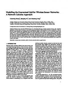
2. System Assumptions For this work we consider the following scenario adapted from [8]. 100 sensors are deployed randomly (albeit distributed uniformly) throughout the region of coverage, in this case a square with coordinates ranging from -100 to +100 as shown in Fig. 1 (L). 100
100 80 loss dB
50 0 -50 -100 -100
60 40 20
-50
0
50
100
0 1 10
3. Gur Game Strategies 3.1. Background Material In the Gur game strategy proposed in [8], sensors operate in three modes: ON, OFF and BASE. ON sensors are active in sending data to the BASE during a given epoch, while OFF sensors are in a standby state. Only one sensor in the network is in BASE mode. All sensors are assumed to have sufficient transmission strength to cover the entire area. As such, understanding the propagation environment will enable an appropriate power level to be selected a priori thereby maximizing system life. Associated with each sensor is a finite, discretetime 2N-state automaton which has N OFF states (-1…N) and N ON states (+1…+N) as shown for the N=3 case in Fig. 2. Sensors move from one state to another based on being rewarded for their behavior (ON-grey or OFF-white) with probability p or punished with probability 1-p. A reward pushes the sensor to a higher state (solid line), i.e., towards ±N. Sensors at edge states (±N) self-loop. A punishment moves the sensor’s state towards the center (dashed line). REWARD
2
10 BASE-active node distance
Figure 1. Example of 100 randomly distribute sensors (L) and propagation loss between BASE and ON sensors (R).
We also assume the sensors are deployed directly on the ground. We model the propagation environment using the log-shadow [10] model with empirically determined parameters for this scenario, (n=3.4, σ=4.7) [11] as shown in Fig. 1 (R). Note, that to date, there has been little additional work in quantifying the propagation environment expected to be incurred by wireless sensor networks [12]. Many authors employ the two-ray model (n=4, σ=0) co-opted from cellular communication analysis [2, 13] Since energy conservation is critical in WSN design and energy use is highly dependent on required RF transmission levels, WSN specific propagation measurements and models require further work. The sensors communicate via single hop to a basestation (BASE) which further relays the information to the next level of nodes (e.g., the network gateway). Our concern herein is to control the number of nodes in this subnet which are actively sensing in any epoch. Note that this hierarchical structure mimics the clusterhead arrangement proposed in the LEACH architecture [14]. In fact, the work herein may be considered as addressing the network control within one cluster. Like LEACH, we will address the problem of sharing the BASE (or clusterhead) responsibilities among sensors on a rotating basis.
-3
-2
-1
1
2
3
PUNISHMENT OFF
ON
Figure 2. Gur game automaton diagram
The referenced work demonstrated that N=3 provides good overall system performance. In addition, we have found that the best network convergence is obtained when all sensors are deployed in State -1; and that, in fact, the network fails to converge to the desired QoS should all sensors be deployed in State +3. Hence, all simulations have assumed N=3 and all sensors are initiated to State -1. Throughout this paper, we compare our strategies with the baseline proposed in [8] using a similar example. Specifically, the control strategy is to maintain 35 active sensors throughout the life of the network. The reward probability is dependent on the number of sensors ON as shown in Fig. 3. and is given for this example by p (ON ) = 0.2 + 0.8 exp( −0.002(ON − 35) 2 ) (1) All sensors, including those that are OFF, listen for reward/punishment information. As implemented, sensors reward/punish themselves based on comparing a locally-generated, uniformly-distributed random
number with the reward probability, p, broadcasted by the BASE at each epoch. Sensors generating numbers less than p are rewarded. 1 0.8 0.6 0.4 0.2 0
0
20
40
60
80
100
Figure 3. Gur game reward function: reward probability p vs. sensors in ON state
3.2. Network life versus sensor reliability In any system one must consider the reliability of its components when ascertaining overall system performance. Thus our question was whether the proposed strategy performed adequately for various levels of sensor reliability. Eq. (1) does not include any information regarding expected sensor life and thus assumes static network resources, which is clearly not the case in WSN. For example, sensors may fail at regular intervals due to low reliability due to costdriven design choices, environmentally caused effects (especially in harsh environments), loss of energy, etc. Thus our strategy modifies p (given by (1)) based on a priori knowledge of the mean expected life of sensors, τ , and the current network life (epoch). pmod (ON) = p (ON) ⋅ exp(−epoch / τ ) (2) We modeled each sensor’s life according to an exponentially generated random variable with means ranging from 50 to 1000 epochs. Network QoS was measured at the end of 100 epochs with results shown in Fig. 4.
showed no performance improvement. Clearly the performance of the modified technique depends greatly on the quality of the a priori knowledge used in (2). As such, these results bode well for investigating adaptive reward/control strategies such as presented in § 4. The modified reward function (2) scales the reward probability downward (or to the left in Fig. 3) as network life increases. The effect is that increasingly sensors become rewarded less for their present behavior and thus causing them to change state more often. This effect is clearly shown in comparing sensor state vs. epoch for the case where expected sensor life τ = 250. From Fig. 5a, we note that at mid-life (epoch=50, center panel), sensors are either in one of the extreme states (±3) or dead as noted by State -4. Note: State +5 indicates the sensor that is currently in the BASE state. 4
4
4
2
2
2
0
0
0
-2
-2
-2
-4
0
50
100
-4
0
50
100
-4
0
50
100
Figure 5a. Sensor state vs. sensor number at epoch 5 (L), 50 (center) and 100 (R) using Eq. (1) – Gur.
In contrast, Fig. 5b shows the result when a time varying strategy is used. Punishing sensors more often (as time progresses) moves sensors towards the center states thus enabling them to switch modes (ON to OFF or OFF to ON) with greater frequency and thereby allowing the control strategy to better adapt to the system dynamics (namely, sensors failing). 4
4
4
2
2
2
0
0
0
-2
-2
-2
sensors active at 100 epochs
40 35 30 25 20 15
-4
10
0
50
100
-4
0
50
100
-4
0
50
100
Figure 5b. Sensor state vs. sensor number at epoch 5 (L), 50 (center) and 100 (R) using Eq. (2) – modified Gur.
5 0 52
99 149 208 245 307 407 512 588 737 816 920 992 e xpe cte d life of individual s e ns ors original
3.3. Network life in energy poor environments
modif ied
Figure 4. Network QoS at 100 epochs for original and modified control Gur game strategies.
From this figure, we draw the following conclusions. First, and as expected, a time dependent strategy performs better for a time-dependent system than a static strategy. Secondly, for systems employing sensors with extremely short life expectancies (less than desired network life), the proposed modified strategy
The results presented above have assumed that a sensor’s failure-rate-function includes running out of energy. However, energy use by a sensor is largely deterministic and will be predominately driven by communication issues, particularly transmission durations and transmission distances. Clearly, the BASE sensor will at any point in time have the highest energy drain of any of the deployed sensors. LEACH rotates BASE responsibility among the sensors to
6
100
4
80
60 gate id
sensor state
2 0
40
-2 20
-4 -6
0
50 sensor no.
100
0
0
50 epoch
100
Figure 6. Sensor state vs. sensor number at end-of-life (L). BASE sensor number vs. network life (R).
The loss of BASE sensors due to running out of energy has an effect of reducing the aggregate life span of sensors below τ =250. To compensate for this, the reward function from Eq. (1) was pmod 2 (ON) = p (ON) ⋅ exp(− K ⋅ epoch / τ ) (3) where K=2 was found empirically to worked well for the scenario considered. In spite of the energy poor system considered and the relatively low reliability of the individual sensors, the proposed control strategy does a reasonable job maintaining QoS over the desired network lifetime as shown in Fig 7. 100
80 no. of sensors
ensure even draw down. However, this methodology requires increased computational complexity. Our strategy simply has the BASE perform its function until it runs out of energy (as denoted by a new State -5 or OUT). In our approach, when a BASE sensor dies, the next sensor to transmit will not be acknowledged. If power control is employed, the sensor will retransmit at full strength to probe the entire coverage area for a potential new BASE. Since this second transmission will also fail to be acknowledged, the sensor will assume BASE responsibilities until it too becomes completely drained. Note that in our method it is possible for some data to be lost. However, we contend that for cost-driven applications not every piece of data will be “mission critical”. We assume the functionality of the BASE is to receive data packets, encapsulate them and for them to the network’s gateway. That is, the BASE does not track where the received data comes from (this reduces the computation and memory requirements for sensors). However, all sensors should be able to determine received power levels. As such, a simple power control strategy could be to append package acknowledgements with a back-off power value. When BASE sensors change, sensors will either (1) need to probe for a new BASE since their transmission levels are now insufficient or (2) will receive new back-off values due to the lower propagation loss between the sensor and the new BASE. The results of employing the BASE assignment strategy are shown in Fig. 6. The left figure shows sensor state at the end of life (epoch=100). From this figure we note that of the original 100 sensors, 18 have run out of energy (State -5), 29 have failed for other reasons (State -4), 33 are ON (State +1, +2 & +3), 19 are OFF (State -1, -2 &-3) and 1 is the current BASE (State +5). The right panel of Fig. 6 shows the BASE sensor’s number as a function of network life. In this case, the BASE station’s life expectancy is very short (~7 epochs) due to the original energy allocation given to each sensor (~200 communication transmissions). Note that the BASE must also acknowledge every other sensor’s data transmission in addition to broadcasting control information.
Lost sensors
Modified Gur
60
40
20
0
Gur 0
20
40
60 epoch
80
100
120
Figure 7. QoS for energy poor environments.
As sensors die off and network life increases, punishments become more frequent. From Fig. 2 we see that thus sensor states will move towards the center. The end result, for both control techniques, is that the number of OFF sensors and the number of ON sensors trend toward each other in addition to declining. Due to the automaton structure sensors will be encouraged to switch modes from ON to OFF and vice versa (noting again, that all sensors receive the same information since the reward is broadcasted). The end result is that only ~50% of the available sensors will be in the ON state when the number of available sensors drops below twice the desired QoS.
4. QoS Control in Random Access Systems Our approach to this QoS problem is to implement control on an individual sensor basis. It should be noted that RF communication energy costs are the significant component in determining sensor life. However there are applications where the duty cycles for transmissions is extremely low, for example, daily logging of environmental parameters such as watershed pollutants. In such applications, the requirement that sensors be listening for control broadcasts will be costly in terms of energy consumption. In fact, some reports [15] indicate the receive functionality consumes nearly as much power at the transmit functionality! As such, we now consider a control strategy the takes full advantage of the low energy aspects of random access
REWARD
p1
p2
p3
PUNISHMENT Figure 8. ACK feedback automaton.
The BASE (keeping a running load count) will determine at each received transmission whether more or less active users are needed. If the running epoch count is too high, the ACK will include a punishment to instruct the sensor to move to a lower state (i.e., to transmit less frequently). With the ACK feedback
scheme, sensors are encouraged individually to modify their state. As such, in a network where the number of available sensors is low, sensors will be encouraged to transmit more frequently and thereby increasing the number of sensors active in the running epoch. Finally, since reward information is tailored to individual sensors, the BASE acknowledgements can be sent at power levels appropriate for the link loss (noting sensors can transmit their power levels along with data) and not at full power as in the broadcast technique. The performance improvement of the proposed ACK feedback technique over the original technique is significant especially towards the latter stages of network life. In Fig. 9, we revisit the limited energy case of § 3.3. The ACK method maintains a QoS of approximately 35 even when the total number of available sensors is 38 at epoch = 150 (of the initial 100, 61 have expired and 1 is the gateway). In contrast, the Gur game method used throughout for comparison maintains a QoS of only p2> p1. For the following simulations, we found that three states produced good results when the probabilities assigned were 1, 0.1 or 0.05, respectively.
Lost sensors
ACK
60
40
20
Gur 0
0
50
100
150
epoch
Figure 9. QoS performance vs. epoch for proposed adaptive scheme and Gur strategy. Network life is extended more than 3x using the adaptive ACK scheme.
The ACK technique requires no a priori knowledge of expected sensor life, as does our Gurbased scheme using Eqs. (2) or (3), and is not sensitive to the number of sensors deployed to be implemented. Fig. 10 (L), demonstrates QoS performance vs. network life for the case where the expected sensor life is reduced to τ =150 (i.e., by 40%). In Fig. 10 (R), the scenario limits the initial distribution to 75 sensors (i.e., a 25% reduction) where the expected life is τ =250. We note in this latter figure that during the final ~10 epochs, all available sensors are ON. The ability of the proposed ACK feedback technique to adapt to changes in the network resources (i.e. number of available sensors) is based on the fact
100
100
80
80 no. of sensors
no. of sensors
that all sensors are in some state of standby. That is, at various random intervals, all sensors will transmit. This operation mode perturbs the network through out its life causing sensors to switch states regularly (Fig. 11 (L)). This is most clearly seen in the case where sensors have infinite life and infinite energy. Fig. 11 (R) indicates that once the Gur game strategy converges on a solution, there is no variability and the reward p is consistently 1 and thus sensors get pushed to the outermost states ±N. However, the premise of this work is that such a scenario is idyllic and thus adaptive techniques are necessary in practice.
60 40 20 0
60 40 20
0
50 epoch
0
100
0
50 epoch
100
100
100
80
80 no. of sensors
no. of sensors
Figure 10. QoS performance for proposed ACK feedback technique with short-life sensors (L) and low initial deployment (R). At epoch = 100, the lines indicate OFF sensors, ON sensors and lost sensors (bottom to top).
60 40 20 0
60 40 20
0
50 epoch
100
0
0
50 epoch
100
Figure 11. QoS performance for proposed ACK feedback (L) and Gur (R) strategies under infinite life and energy conditions. At epoch = 100, the lines indicate OFF sensors (top) and ON sensors (bottom).
5. Conclusions and Future Work In this paper, we have presented results of an initial investigation that builds a recently proposed means of controlling QoS in a hierarchically-structured wireless sensor network. The method utilizes a strategy of rewards and punishments which control the operating state of sensors. One result, albeit intuitively obvious, is that in a network where the available resources degrade over time, one can not expect to successfully employ a static control strategy. We also present a new WSN QoS control strategy that not only extends network life in harsh, energy constrained environments but also takes advantage of low-energy random access protocols. While the methodology is not suitable for high-performance, bandwidth limited applications; we
contend a wide range of general sensing applications can take full advantage of the methods proposed herein. Future work should be performed in rigorously defining the interplay between the control strategy and the underlying network parameters including, sensor reliability, true energy costs, propagation environment and, naturally, desired QoS. Herein, we have verified through simulation, that these parameters do affect overall network life, but simulation does not give us the insight of an analytical solution. With the work presented herein, the author hopes to have contributed to this field by identifying some promising areas for continued investigation. [1] Pottie, G. and W. Kaiser, “Wireless integrated network sensors,” Comm. ACM, 43(5):51-58, May 2000. [2] Estrin, D., L. Girod, G. Pottie and M. Srivastava, “Instrumenting the world with wireless sensor networks,” In Proc. Int'l Conf. Acoustics, Speech and Signal Processing (ICASSP 2001). [3] MIT Technology Review, “10 emerging technologies that will change the world,” MIT Technology Review, Feb. 2003. [4] Auster, B., “Waging war,” ASEE Prism, Feb. 2002, 19-23. [5] Mainwaring, A, et al, “Wireless sensor network for habitat monitoring,” Wireless Sensor Networks and Applications (WSNA 2002), Atlanta, GA, Sept. 28. [6] West, B., et al, “Wireless sensor networks for dense spatio-temporal monitoring of the environment: a case for integrated circuit, system, and network design,” Proc. IEEE CAS Workshop on Wireless Comm. & Networking, Aug 2001. [7] Perillo, M. and W. Heinzelman, “Providing application QoS through intelligent sensor management,” 1st Sensor Network Protocols and Applications Workshop (SNPA 2003), Anchorage, AK, May 11. [8] Iyer, R. and L. Kleinrock, “QoS Control for Sensor Networks,” IEEE International Comm. Conference (ICC 2003), Anchorage, AK, May 11-15. [9] Clare, L., J. Agre and T-S Yan, “Considerations on communication network protocols in deep space,” IEEE Proc. Aerospace Conf., Big Sky, MT. Mar. 2001. [10] Rappaport, T., Wireless communications: principles and practice, Prentice Hall, New Jersey, 1996. [11] Fanimokun, A. and J. Frolik, “Effects of natural propagation environments on wireless sensor network coverage area,” 2003 IEEE Southeastern Symposium on System Theory (SSST03), Morgantown, WV, Mar. 16-18. [12] Sohrabi, K., B. Manriquezand G. Pottie, “Near ground wideband channel measurement in 800-1000 MHz,” 49th IEEE Vehicular Tech. Conference, Vol. 1, 16-20 May 1999. [13] Krishnamachari, B., Y. Mourtada and S. Wicker, “The energy-robustness tradeoff for routing in wireless sensor networks,” IEEE International Comm. Conference (ICC03), Anchorage, AK, May 11-15. [14] Heinzelman, W., L. Chadrakasan and H. Balakrshnan, “An Application-Specific Protocol Architecture for Wireless Microsensor Networks,” IEEE Trans. on Wireless Comm., Vol. 1, No. 4, Oct. 2002. [15] Raghunathan, V., C. Schurgers, S. Park and M. Srivastava, “Energy-aware wireless microsensor networks,” IEEE Signal Processing Mag., Vol. 19, No. 2, Mar. 2002.