Oct 29, 2011 - Given an input data matrix, NMF finds an approximation that is factorized into a ... mating a hidden Markov chain, and graph matching. In the rest of ..... 9 http://www.cise.ufl.edu/research/sparse/matrices/index.html. Z. Yang, E.
Pattern Recognition 45 (2012) 1500–1510
Contents lists available at SciVerse ScienceDirect
Pattern Recognition journal homepage: www.elsevier.com/locate/pr
Quadratic nonnegative matrix factorization Zhirong Yang n, Erkki Oja Aalto University, Department of Information and Computer Science, P.O. Box 15400, FI-00076 Aalto, Finland
a r t i c l e i n f o
a b s t r a c t
Article history: Received 23 February 2011 Received in revised form 27 September 2011 Accepted 21 October 2011 Available online 29 October 2011
In Nonnegative Matrix Factorization (NMF), a nonnegative matrix is approximated by a product of lower-rank factorizing matrices. Most NMF methods assume that each factorizing matrix appears only once in the approximation, thus the approximation is linear in the factorizing matrices. We present a new class of approximative NMF methods, called Quadratic Nonnegative Matrix Factorization (QNMF), where some factorizing matrices occur twice in the approximation. We demonstrate QNMF solutions to four potential pattern recognition problems in graph partitioning, two-way clustering, estimating hidden Markov chains, and graph matching. We derive multiplicative algorithms that monotonically decrease the approximation error under a variety of measures. We also present extensions in which one of the factorizing matrices is constrained to be orthogonal or stochastic. Empirical studies show that for certain application scenarios, QNMF is more advantageous than other existing nonnegative matrix factorization methods. & 2011 Elsevier Ltd. All rights reserved.
Keywords: Nonnegative matrix factorization Multiplicative update Stochasticity Orthogonality Clustering Graph partitioning Hidden Markov chain model Graph matching
1. Introduction Extensive research on Nonnegative Matrix Factorization (NMF) has emerged in recent years (e.g. [1–6]). NMF has found a variety of applications in machine learning, signal processing, pattern recognition, data mining, information retrieval, etc. (e.g. [7–11]). Given an input data matrix, NMF finds an approximation that is factorized into a product of lower-rank matrices, some of which are constrained to be nonnegative. The approximation error can be measured by a variety of divergences between the input and its approximation (e.g. [12–14,6]), and the factorization can take a number of different forms (e.g. [15–17]). In most existing NMF methods, each factorizing matrix appears only once in the approximation. We call them linear NMF because the approximation is linear with respect to each factorizing matrix. However, such linearity assumption does not hold in some important real-world problems. A typical example is graph matching, when it is presented as a matrix factorizing problem, as pointed out by Ding et al. [18]. If two graphs are represented by their adjacency matrices A and B, then they are isomorphic if and only if a permutation matrix P can be found such that A�PBPT ¼ 0. Minimizing the norm or some other suitable error measure of the left-hand side with respect to P,
n
Corresponding author. Tel.: þ358 414869473. E-mail addresses: zhirong.yang@aalto.fi (Z. Yang), erkki.oja@aalto.fi (E. Oja).
0031-3203/$ - see front matter & 2011 Elsevier Ltd. All rights reserved. doi:10.1016/j.patcog.2011.10.014
with suitable constraints, reduces the problem to an NMF problem. The approximation is now quadratic in P. Another example is clustering: if X is a matrix whose n columns need to be clustered into r clusters, then the classical K-means objective function can be written as [19] J 1 ¼ Tr ðXT XÞ�TrðUT XT XUÞ where U is the (n � r) binary cluster indicator matrix. The global minimum with respect to U gives the optimal clustering. It was shown in [20] that minimizing J 2 ¼ JXT �WWT XT J2Frobenius with respect to an orthogonal and nonnegative matrix W gives the same solution, except for the binary constraint. This is another NMF problem where the approximation is quadratic in W. Although the need of quadratic factorizations has been occasionally addressed in the literature (e.g. [21,18,17]), there has been no systematic study of higher-order NMF. A general way to obtain efficient optimization algorithms is lacking as well. In this paper we focus on a class of NMF methods where some factorizing matrices occur twice in the approximation. We call these methods Quadratic Nonnegative Matrix Factorization (QNMF). Our major contributions are highlighted as follows: (1) QNMF objectives that are composed of different factorization forms and various approximation error measures are formulated. (2) Solving a QNMF problem is generally more difficult than the linear ones, because the former usually involves a higher-degree objective function with respect to the doubly occurring factorizing matrices. In [22], we recently introduced a general approach for deriving multiplicative update rules for NMF, based on most commonly used approximation error measures. We now apply it
Z. Yang, E. Oja / Pattern Recognition 45 (2012) 1500–1510
to more general QNMF factorizations. Iterative algorithms that utilize the derived rules can all be shown to guarantee monotonic decrease, thus convergence, of the objective function. (3) We present techniques for extending the algorithms to easily accommodate the stochasticity or orthogonality constraint, needed for such applications as estimating a hidden Markov chain, clustering or graph matching. (4) In addition to the advantages in clustering, already shown in our previous publication [20], we demonstrate that the proposed QNMF algorithms outperform the existing NMF implementations in graph partitioning, two-way clustering, estimating a hidden Markov chain, and graph matching. In the rest of the paper, we first briefly review the nonnegative matrix factorization problem and related work in Section 2. Next we formulate the Quadratic Nonnegative Matrix Factorization problem in Section 3, with its multiplicative optimization algorithms, learning with the stochasticity and orthogonality constraints given in Section 4. Section 5 presents experimental results, including comparisons between QNMF and other stateof-the-art NMF methods for four selected applications, as well as the demonstration of accelerated and online QNMF. Some conclusions and future perspectives are given in Section 6.
1501
such as L1- or L2-norm have been used for achieving sparseness or smoothness (e.g. [24,3,8]). Orthogonality combined with nonnegativity can significantly enhance the part-based representation or category indication (e.g. [16,25,4,26,20]).
3. Quadratic nonnegative matrix factorization In most existing NMF approaches, the factorizing matrices FðqÞ b as a in Eq. (1) are all different, and thus the approximation X function of them is linear. However, there are useful cases where some matrices appear more than once in the approximation. In this paper we consider the case that some of them may occur T twice, or formally, FðsÞ ¼ FðtÞ for a number of non-overlapping pairs fs,tg and 1 r s ot r Q . We call such a problem and its solution Quadratic Nonnegative Matrix Factorization (QNMF) b as a function is quadratic to each twice appearing because X factorizing matrix.2 To avoid notational clutter, we focus on the case where the input matrix and all factorizing matrices in the approximation are nonnegative, while our discussion can easily be extended to the cases where some matrices may contain negative entries by using the decomposition technique presented in [17].
2. Related work Given an input data matrix X A Rm�n , Nonnegative Matrix b which can be Factorization (NMF) finds an approximation X factorized into a product of matrices b¼ X�X
Q Y
FðqÞ
ð1Þ
q¼1
and some of these matrices are constrained to be nonnegative. The dimensions of the factorizing matrices Fð1Þ , . . . , FðQ Þ are m � r 1 , r 1 � r 2 , . . . , r Q �1 � n, respectively. Usually r 1 , . . . , r Q�1 are much smaller than m or n. In this way the factorization represents the data in a more compact way and thus favors certain applications. The difference between the input matrix X and its approximab can be measured by a variety of divergences, for which tion X theoretically convergent multiplicative algorithms of NMF have been proposed.1 Originally, NMF is based on the Euclidean distance or I-divergence (non-normalized Kullback–Leibler divergence) [1,2]. These two measures were later unified by using the b-divergence [12]. Alternatively, Cichocki et al. [14] generalized NMF from I-divergence to the whole family of a-divergences. NMF has been further extended to a even broader class called Bregman divergence, for many cases of which a general convergence proof can be found [13]. In addition to separable ones, divergences that are non-separable with respect to the matrix entries such as the g-divergence and Re´nyi divergence can also be employed by NMF [11]. Many other divergences for measuring the approximation error in NMF exist, although they may lack theoretically convergent algorithms. In its original form [1,2], the NMF approximation is factorized into two matrices (Q¼2). Later the factorization was generalized to three factors (e.g. [23,15–17]). Note that the input matrix and some factorizing matrices are not necessarily nonnegative, (e.g. Semi-NMF in [17]). Also, one of the factorizing matrix can be the input matrix itself, for example, the Convex NMF [17]. Besides the nonnegativity, various constraints or regularizations can be imposed on the factorizing matrices. Matrix norms 1 Unless otherwise stated, the term ‘‘convergence’’ in this paper generally refers to the objective function convergence or, equivalently, the monotonic decrease of the NMF approximation error.
3.1. Factorization forms To begin with, let us consider the QNMF objective with only one doubly occurring matrix W. The general approximating factorization form is given by b ¼ AWBWT C, X
ð2Þ
where we merge the products of the other, linearly appearing factorizing matrices into single symbols. It is also possible that matrix A, B, and/or C is the identity matrix and thus vanishes from the expansion. Here we focus on the optimization over W, as learning the matrices that occur only once can be solved by using the conventional NMF methods of alternative optimization over each matrix separately [11]. The above factorization form unifies all previously suggested QNMF objectives. For example, it becomes the Projective Nonnegative Matrix Factorization (PNMF) when A ¼ B ¼ I and C ¼ X, which was first introduced by Yuan and Oja [21] and later extended by Yang et al. [25,27,20]. This factorized form is also named Clustering NMF in [17] as a constrained case of Convex NMF. Even without any explicit orthogonality constraint, the matrix W obtained by using PNMF is highly orthogonal and can thus serve two purposes: (1) when the columns of X are samples, W can be seen as the basis for part-based representations, and (2) when the rows of X are samples, W can be used as a cluster indicator matrix. If X is a square matrix and A ¼ C ¼ I, the factorization can be used in two major scenarios if the learned W is highly orthogonal. (1) When B is much smaller than X, the three-factor approximation corresponds to a blockwise representation of X [23,28]. If B is diagonal, then the representation becomes diagonal blockwise, or a partition. In the extreme case B ¼ I, the factorization reduces to b ¼ WWT the Symmetric Nonnegative Matrix Factorization (SNMF) X [16]. (2) When X and B are of the same size, the learned W with the constraint WT W ¼ I approximates a permutation matrix and thus QNMF can be used for learning order of relational data, for example, graph matching [18]. Alternatively, under the constraint that W has column-wise unitary sums, the solution of such a 2 Though equality without matrix transpose, namely FðsÞ ¼ FðtÞ , is also possible, to our knowledge there are no corresponding real-world applications.
1502
Z. Yang, E. Oja / Pattern Recognition 45 (2012) 1500–1510
QNMF problem provides parameter estimation of hidden Markov chains (see Section 5.3). The factorization form in Eq. (2) also generalizes the concepts of Asymmetric Quadratic Nonnegative Matrix Factorization b ¼ WWT C and Symmetric Quadratic Nonnegative Matrix (AQNMF) X b ¼ WBWT in our previous work [22]. Factorization (SQNMF) X Note that the factorization form in Eq. (2) is completely general: it can be recursively applied to the cases where there are more than one factorizing matrices appearing quadratically in the approximation. For example, the case A ¼ CT ¼ U yields b ¼ WWT XUUT . b ¼ UWBWT UT , and A ¼ B ¼ I, C ¼ XUUT yields X X An application of the latter example is shown in Section 5.2, where the solution of such a QNMF problem can be used to group the rows and columns of X simultaneously. This is particularly useful for the biclustering or coclustering problem. These factorizing forms can be further generalized to any number of factorizing matrices. In such cases we employ alternative optimization over each doubly occurring matrix. It is important to notice that quadratic NMF problems are not special cases of linear NMF. The optimization methods of the latter generally cannot be extended to QNMF. For linear NMF, the factorizing matrices are different variables and the approximation error can alternatively be minimized over one of them while keeping the others constant. In contrast, the optimization of QNMF is more comprehensive because matrices in two places vary simultaneously, which leads to higher-order objectives. For example, given the squared Frobenius norm (Euclidean distance) as approximation error measure, the objective of linear NMF JX�WHJ2F is quadratic with respect to W and H, whereas the PNMF objective JX�WWXJ2F is quartic with respect to W. Minimizing such a fourth-order objective with the nonnegativity constraint is considerably more challenging than minimizing a quadratic function. In contrast to the rich selection of approximation error measures for linear NMF, there is little research on such measures for quadratic NMF. In this paper we show that QNMF can be built on a very wide class of dissimilarity measures, quite as rich as those for linear NMF. Furthermore, as long as the QNMF objective can be expressed in a generalized polynomial form described below, we show that there always exists a multiplicative algorithm that theoretically guarantees convergence, or the monotonic decrease of the objective function, in each iteration. ~ from its In the rest of the paper, we distinguish the variable W ~ ¼ AWB ~ W ~ T C to denote the current estimate W. We write X ~ and X b ¼ AWBWT C approximation that contains the variable W, for the current estimate (constant). 3.2. Deriving multiplicative algorithms Multiplicative updates have been commonly used for optimizing NMF objectives. In each epoch, a factorizing matrix is updated by elementwise multiplication with a nonnegative matrix which can easily be obtained from the gradient. The multiplicative algorithms have a couple of advantages over the conventional additive gradient descent approach. Firstly, they naturally maintain the nonnegativity of the factorizing matrices without any extra projection steps. Secondly, the fixed-point algorithm that iteratively applies the update rule requires no user-specified parameters such as the learning step size, which facilitates its implementation and applications. Although some heuristic connections to conventional additive update rules exist [2,25], they cannot theoretically justify the objective function convergence. The rigorous convergence proof, or theoretical guarantee of monotonic decrease of the objective function, focusses on
minimizing a certain auxiliary upper-bounding function which is defined as follows. GðW,UÞ is called an auxiliary function if it is a tight upper bound of the objective function J ðWÞ, i.e. GðW,UÞ Z J ðWÞ, and GðW,WÞ ¼ J ðWÞ for any W and U. Define ~ Wnew ¼ arg min GðW,WÞ: ~ W
ð3Þ
By construction, J ðWÞ ¼ GðW,WÞ Z GðWnew ,WÞ Z GðWnew ,Wnew Þ ¼ J ðWnew Þ, where the first inequality is the result of minimization and the second comes from the upper bound. Iteratively applying the update rule (3) thus results in a monotonically decreasing sequence of J . Besides the tight upper bound, it is often desired that the minimization (3) has a closed-form solution. In particu~ ¼ 0 should lead to the iterative update rule in lar, setting @G=@W analysis. The construction of such an auxiliary function, however, has not been a trivial task so far. In [22], we recently derived the convergent multiplicative update rules for a wide class of divergences for the NMF problem. For conciseness, we repeat the central steps here but for details refer to [22]. Let us first generalize the definitions of monomials and polynomials: a monomial with real-valued exponent, or shortly monomial, of the scalar variable z is of the form azb where a and b can take any real value, without restriction to nonnegative integers. A sum of a (finite) number of monomials is called a (finite) generalized polynomial. This form of expression has two nice properties: (1) individual monomials, denoted by azb, are either convex or concave with respect to z and thus can easily be upper-bounded; (2) an exponential is multiplicatively decomposable, i.e. ðxyÞa ¼ xa ya , which is critical in deriving the multiplicative update rule. Note that we unify the logarithm function that is involved in many information-theoretic divergences to our generalized polynomial form by using the logarithm limit ln z ¼ limþ E-0
zE �1
E
:
ð4Þ
Notice that limits in 0 þ and 0 � are the same. We use the former to remove the convexity ambiguity. In this way, the logarithm can be decomposed into two monomials where the first contains an infinitesimally small positive exponent. Next, we show that the auxiliary upper-bounding function always exists as long as the approximation objective function can be expressed in the finite generalized polynomial form. This is formalized by the following theorem in our previous work [22]. Theorem 1. Assume Od ðzÞ ¼ rd � zwd , and rd , wd , gdij and fd are ~ If the approximation error has the form constants independent of W. 0 1 p m X n X X fd b ¼ b A þ constant, DðXJXÞ ð5Þ Od @ g dij X ij d¼1
i¼1j¼1
then there are real numbers cmax and cmin (cmax 4 cmin ) such that ! ! ~ ik cmax þ W ik W ~ ik cmin � X W ik W ~ GðW,WÞ ¼ rik � rik þ constant cmax W ik cmin W ik ik ð6Þ ~ ~ There is an auxiliary upper-bounding function of J ðWÞ9DðXJ XÞ. r þ and r� denote the sums of positive and unsigned negative terms þ � ~ ~ ~ of r ¼ @J ðWÞ=@ W9 (i.e. r ¼ r �r ), respectively. W¼W The theorem proof, or the construction procedure of the auxiliary function is summarized in the following procedure: (1) write the objective function in the form of finite generalized polynomials given by Eq. (5); use the logarithm limit Eq. (4) when necessary; (2) if the objective is not a separable sum over i and j, i.e. there is wd a 1, derive a separable upper-bound of the
Z. Yang, E. Oja / Pattern Recognition 45 (2012) 1500–1510
objective using the concavity or convexity inequality on Od ; (3) upper bound individual monomials according to their concavity/ convexity and leading signs; (4) if there are more than two upperbounds with distinct exponents, combine them into two monomials according to their exponents and leading signs. The derivation details are similar to those given in our previous work [22] and thus omitted here. Taking the derivative of the auxiliary function with respect to ~ leads to W ! ! ~ ~ ik cmax �1 þ ~ ik cmin �1 � @GðW,WÞ W W ¼ r � rik : ð7Þ ik ~ ik W ik W ik @W As stated above, setting this to zero gives the iterative update rule, which results in a monotonically decreasing, hence convergent, sequence of J ðWÞ. In most cases, this multiplicative update rule has the form !Z W new ¼ W ik ik
r�ik rikþ
,
ð8Þ
where Z ¼ 1=ðcmax �cmin Þ. An exception, for example the dual I-divergence, happens when the logarithm limit is applied and limE-0 þ ðcmax �cmin Þ ¼ 0. In this case the limit of the derivative Eq. (7) has the form 00 and can be resolved by using L’Hˆopital’s rule to obtain the limit before setting it to zero. The finite generalized polynomial form Eq. (5) covers most commonly used dissimilarity measures. Here we present the multiplicative update rules for QNMF based on a-divergence, b-divergence, g-divergence and Re´nyi divergence. These families include, for example, the squared Euclidean distance (b ¼ 1), Hellinger distance (a ¼ 0:5), w2 -divergence (a ¼ 2), I-divergence (a-1 or b-0), dual I-divergence (a-0), Itakura–Saito divergence (b-�1) and Kullback–Leibler divergence (g-0 or r-1). Though not presented here, more QNMF objectives, for example the additive hybrids of the above divergences, as well as many other unnamed Csisza´r divergences and Bregman divergences, can be easily derived using the proposed principle. In general, the multiplicative update rules take the following form " #Z ðAT QCT WBT þ CQ T AWBÞik new W ik ¼ W ik �y , ð9Þ ðAT PCT WBT þ CPT AWBÞik where P, Q , y, and Z are specified in Table 1. For example, the rule for QNMF X � WBWT based on the squared Euclidean distance (b-1) reads " #1=4 ðXWBT þXT WBÞik W new ¼ W ik : ik ðWBWT WBT þWBT WT WBÞik
1503
As an exception, the update rules for the dual I-divergence takes a different form " # 1 ðAT QCT WBT þ CQ T AWBÞik new W ik ¼ W ik exp 2 ðAT PCT WBT þ CPT AWBÞik b ij Þ. In practice, iteratively applying with P ij ¼ 1 and Q ij ¼ lnðX ij =X the above update rules except the dual-I case can also achieve K.K.T. optimality asymptotically [22]. Multiplicative algorithms using an identical update rule throughout the iterations are simple to implement. However, the exponent Z that remains constant is often conservative (too small) in practice. This can be accelerated by using a more aggressive choice of the exponent, which adaptively changes during the iterations. A simple strategy is to increase the exponent steadily if the new objective is smaller than the old one and otherwise shrink back to the safe choice, Z. We find that such a strategy can significantly speed up the convergence while still maintaining the monotonicity of the updates [22]. For very large data matrices, there are scalable implementations of QNMF for the case when the approximation error is the squared Euclidean distance. An online learning algorithm of PNMF was presented in our previous work [29], where we do not need to operate on the whole data matrix but only on a small intermediate variable instead. The resulting algorithm not only has low memory cost but also runs faster than the batch version for large datasets.
4. Constrained QNMF NMF objectives are often accompanied with a set of constraints. The manifolds induced by these constraints intersect the nonnegative quadrant and form an extensive and non-smooth function domain, which makes the optimization difficult. Conventional optimization approaches which operate in such domains only work for a few particular cases of linear NMF but seldom succeed for quadratic NMF problems. Alternatively, we adopt a relaxation technique to solve the constrained QNMF problems: first we attach the (soft) constraints to the objective as regularization terms; next we write a multiplicative update rule for the augmented objective, where the Lagrangian multipliers are solved by using the K.K.T. conditions; finally putting back the multipliers we obtain new update rules with the (soft) constraints incorporated. A similar idea was also employed by Ding et al. [16]. We call the resulting algorithm iterative Lagrangian solution of the constrained QNMF problem. Such an algorithm jointly minimizes the QNMF approximation error and forces the factorizing matrices to approach the constraint manifold. In what follows, we show how to get such a solution for QNMF with the stochasticity or orthogonality constraint. 4.1. Stochastic matrices
Table 1 Notations in the multiplicative update rules of QNMF examples, where b ¼ AWBWT C. X Divergence
Pij
a-Divergence
1
b-Divergence
bb X ij
g-Divergence
g
Re´nyi divergence
b X ij 1
Qij
Z
y
b �a X aij X ij
1
b�1
1
g�1
P bgþ1 ab X ab bg ab X ab X ab P b ab X ab P r b 1�r X ab ab X ab
b X ij X ij
b X ij X ij
b �r X rij X ij
P
1=ð2aÞ for a 4 1 1=2 for 0 o a o 1 1=ð2a�2Þ for a o 0 1=ð2 þ 2bÞ for b 4 0 1=ð2�2bÞ for b o 0 1=ð2 þ 2gÞ for g 4 0 1=ð2�2gÞ for g o 0 1=ð2rÞ for r 4 1 1=2 for 0 o r o 1
Nonnegative matrices are often used to represent probabilities, where all or a part of the matrix elements must sum up to one. For concreteness we only focus on the case of a left stochastic P matrix with column-wise unitary sum, i.e. i W ik ¼ 1, while the same method can easily be extended to row-wise constraints (right stochastic matrix) or matrix-wise constraints (doubly stochastic matrix). A general principle that incorporates the stochasticity constraint to an existing convergent QNMF algorithm is given by the following theorem. ~ to be minimized can Theorem 2. Suppose a QNMF objective J ðWÞ ~ be upper-bounded by the auxiliary function GðW,WÞ in the form of Eq. (6), whose gradient with respect to W is given in Eq. (7). Introducing a set of Lagrangian multipliers flk g, the augmented
1504
Z. Yang, E. Oja / Pattern Recognition 45 (2012) 1500–1510
~ þ P lk ð1�P W ik Þ is non-increasing under objective LðW, kÞ ¼ J ðWÞ k i the update rule " #s P þ r�ik þ a rak W ak ¼ W , ð10Þ W new P ik ik rikþ þ a r�ak W ak where s ¼ 1=½maxðcmax ,1Þ�minðcmin ,1Þ�. The proof is given in Appendix A. Note that the above reforming principle also includes the dual-I divergence case where maxðcmax ,1Þ�minðcmin ,1Þ ¼ 1 or s ¼ 1. The inclusion also holds in the following principle for the orthogonality constraint. 4.2. Orthogonal matrices Orthogonality is another frequently used constraint in NMF (see e.g. [16,18,25,4,20]) because a nonnegative orthogonal matrix has only one non-zero entry in each row. In this way the matrix can serve as a membership indicator in learning problems such as clustering or classification. Strict orthogonality is however of little interest in NMF because the optimization problem remains discrete and often NP-hard. Relaxation is therefore needed, as long as there is only one large non-zero entry in each row of the resulting W while the other entries are close to zero. An approximative orthogonal matrix is then obtained by simple thresholding and rescaling. Here we present a general principle that incorporates the orthogonality constraint to a theoretically convergent QNMF algorithm. In Appendix B we have proven the following results. ~ to be minimized can Theorem 3. Suppose a QNMF objective J ðWÞ ~ be upper-bounded by the auxiliary function GðW,WÞ in the form of Eq. (6), whose gradient with respect to W is given in Eq. (7). Introducing a set of Lagrangian multipliers fLkl g, the augmented ~ þ TrðKðI�W ~ T WÞÞ ~ is non-increasing under objective LðW, KÞ ¼ J ðWÞ the update rule " #s ðr� þWWT r þ Þik new , ð11Þ W ik ¼ W ik þ � ðr þ WWT r Þik where s ¼ 1=½maxðcmax ,2Þ�minðcmin ,0Þ�. Corollary 4. If K þ ¼ 12WT r is positive semi-definite, then s ¼ 1=½maxðcmax ,2Þ�minðcmin ,1Þ� in Eq. (11). þ
Our derivation of the multiplicative rules for learning nonnegative projections is based on the Lagrangian approach. That is, one should apply WT W ¼ I, one of the K.K.T. conditions, to simplify the resulting multiplicative update rule after transforming Eq. (8) to its orthogonal counterpart Eq. (11). Furthermore, removing duplicate terms that appear in both numerator and denominator in practice will lead to faster convergent update rule because (aþc)/(bþc) is closer to one than a/b for a,b,c 4 0. Although with highly orthogonal results, it is important to notice that W never exactly reaches the Stiefel or Grassmann manifold during the optimization if it is initialized with positive entries. Therefore the reforming principle using natural gradients in such manifolds (e.g. [26,4]) must be seen as an approximation.
5. Experiments Quadratic nonnegative matrix factorization can be applied to a variety of learning problems. Extensive empirical studies of PNMF, a special case of QNMF, for feature extraction and clustering have been provided in [21,25,20]. In this paper we demonstrate four new example applications. The first one employs PNMF for grouping the nodes of a graph; the second one applies a two-sided QNMF to achieve two-way clustering; the third one uses QNMF with the stochasticity constraint to estimate the
parameters in hidden Markov chains; and the fourth application uses QNMF with the orthogonality constraint for finding node correspondence of two graphs. The following publicly available datasets have been used in our experiments: Newman’s collection,3 the Pajek database,4 the 3Conference graph,5 the webkb text dataset,6 the top 58112 English words,7 the GenBank database,8 and the University of Florida Sparse Matrix Collection.9 5.1. Graph partitioning Given an undirected graph, the graph partitioning problem is to divide the graph vertices into several disjoint subsets, such that there are relatively few connections between the subsets. The optimization of many graph partitioning objectives, for example, minimizing the number of removed edges in partitioning, is NP-hard due to the complexity of algorithms in a discrete space. It is therefore advantageous to employ a continuous approximation of the objectives, which enables the development of efficient gradient descent—type optimization algorithms by using differential calculus. Suppose the connections in the graph are represented by a real-valued N � N affinity matrix A, whose element Aij gives the weight of the edge connecting vertices i,j. A classical approximation approach is spectral clustering (e.g. [30]) which minimizes TrfUT ðD�AÞUg subject to UT DU ¼ I, where D is a diagonal matrix P with Dii ¼ j Aij . Though the problem has a closed form solution by using singular value decomposition, the resulting U may contain negative entries and thus cannot directly be used as an indicator for more than two clusters. An extra step that projects U to the positive quadrant is needed [31]. Ding et al. [18] presented the Nonnegative Spectral Clustering (NSC) method by introducing the nonnegativity constraint. They derived a multiplicative update rule as an iterative Lagrangian solution that jointly minimizes TrfUT ðD�AÞUg and forces U to approach the manifold specified by UT DU ¼ I and U Z0. We can connect the NSC problem to the PNMF approach. Rewriting W ¼ D1=2 U, which does not change the cluster indication because D is diagonal and positive, the NSC problem becomes maximization of TrfWT ðD�1=2 AD�1=2 ÞWg over nonnegative W and subject to WT W ¼ I. This is a nonnegative PCA problem which can be solved by PNMF [25,20]. Furthermore, we can replace D�1=2 AD�1=2 with some other symmetric matrices or kernel matrices. A good kernel can enhance the clustering effect of the graph and yield better partitioning results. Here we use a nonparametric kernel called random-walk kernel that minimizes the combinatorial formulation of the Dirichlet integral [32–34]. In brief, the kernel is obtained by symmetrizing the solution of the following equation: ð2D�AÞB ¼ A. Consider the reproducing Hilbert space induced by the kernel K ¼ ðB þ BT Þ=2 whose entries P �1 i 1 are nonnegative because B ¼ ð2D�AÞ�1 A ¼ 12 D�1 1 Þ A. i ¼ 0 ð2 AD The graph partitioning problem can thus be solved by applying kernel PNMF [20] in the implicit feature space to minimize JUðXÞT � WWT UðXÞT J2F subject to WZ 0, where K ¼ UðXÞT UðXÞ. The convergent update rule of kernel PNMF derived from the proposed principle is " #1=3 ð2KWÞik ¼ W : W new ik ik ðWWT KW þKWWT WÞik
3 4 5 6 7 8 9
http://www-personal.umich.edu/ � mejn/netdata/ http://vlado.fmf.uni-lj.si/pub/networks/data/ http://users.ics.tkk.fi/rozyang/3conf/ http://www.cs.cmu.edu/afs/cs.cmu.edu/project/theo-20/www/data/ http://www.mieliestronk.com/wordlist.html http://www.ncbi.nlm.nih.gov/genbank/ http://www.cise.ufl.edu/research/sparse/matrices/index.html
Z. Yang, E. Oja / Pattern Recognition 45 (2012) 1500–1510
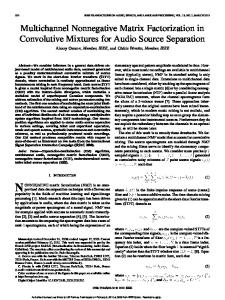
We have compared the nonnegative spectral clustering and our kernel PNMF methods on four graphs: (1) Korea, a communication network of 39 women of two classes in Korea about family planning. (2) WorldCities, a dataset consisting of the service values (indicating the importance of a city in the office network of a firm) of 100 global advanced producer service firms over 315 world cities. The firms are grouped into six categories: accountancy, advertising, banking/finance, law, insurance and management consultancy. (3) PolBlogs, a network of weblogs on US politics, with 1224 nodes. (4) 3Conference, the coauthorship network in three conferences SIGIR, ICML, and ICCV from 2002 to 2007. There are 2817 authors, 14 048 edges in total. The value on each edge represents the number of papers that two authors have coauthored. The first three datasets are gathered from Newman’s collection (see footnote 3) and the Pajek database (see footnote 4). The 3Conference graph is available at the authors’ website (see footnote 5). We have computed the purities of the resulting partitions by using the ground truth class information: given r partitions and q P classes, purity ¼ ð1=NÞ rk ¼ 1 max1 r l r q Nlk , where Nlk is the number of vertices in the partition k that belong to ground-truth class l. A larger purity in general corresponds to better clustering result. For each dataset, we repeated the compared methods 100 times with different random initializations and recorded the purities, whose means and standard deviations are illustrated in Fig. 1. For small graphs Korea and WorldCities, kernel PNMF, or Nonnegative kernel PCA, is at the same level or slightly better than the nonnegative spectral clustering method. For larger graphs PolBlogs and 3Conference, kernel PNMF is significantly superior with much higher clustering purities. The computational cost of both NSC and kernel PNMF is OðN2 rÞ per iteration. We have performed the above experiments using Matlab R2010b software on a personal computer with Intel Core i7 CPU, 8 G memory and Ubuntu 10 operating system. For small graphs such as Korea and WorldCities, the algorithms converged within a few seconds. For larger graphs such as PolBlogs and 3Conference, they converged within 10–15 min.
5.2. Two-way clustering Biclustering, coclustering or two-way clustering is a data mining problem which requires simultaneous clustering of matrix rows and columns. Here we demonstrate an application of QNMF for finding biclusters in which the matrix entries have similar
1 0.9
values. A good biclustering of this kind should generate a blockwise visualization of the matrix when the rows and columns are ordered by their bicluster indices. Two-way clustering has previously been addressed by the linear NMF methods (e.g. [8]). Given the factorization of the input matrix X � WH, the bicluster index for each row of X is determined by the index of maximal entry in each row of W. The bicluster index for columns are likewise obtained. The biclustering problem has also been attacked by three-factor linear NMF X � LSRT with the orthogonality constraint on L and R. For tri-factorizations, Ding et al. [16] gave a multiplicative algorithm called BiOR-NM3F when the approximation error is measured by the squared Euclidean distance. However, when this method is extended to other divergences such as the I-divergence, it is often stuck in trivial local minima where S tends to be smooth or even uniform because of the sparsity of L and R [15]. An extra constraint on S is therefore needed. Here we propose to use a QNMF formulation for the biclustering problem: X � LLT XRRT . Compared with the BiOR-NM3F approximation, here we constrain the middle factorizing matrix S to be LT XR. The resulting two-sided QNMF objectives can be optimized by alternating the one-sided algorithms, that is, interleaving optimizations of X � LLT YðRÞ with YðRÞ ¼ XRRT fixed and X � YðLÞ RRT with YðLÞ ¼ LLT X fixed. The bicluster indices of rows and columns are given by taking the maximum of each row in L and R. We call the new method Biclustering QNMF (Bi-QNMF) or Two-way QNMF. We have compared Bi-QNMF with linear NMF based on the I-divergence and BiOR-NM3F for two-way clustering on both synthetic and real-world data. To our knowledge, BiOR-NM3F is implemented only for the squared Euclidean distance. For comparison, we apply the same development procedure by [16] (see also Section 4.2) to obtain the multiplicative update rules for the I-divergence, which we denote by BiOR-NM3F-I. Firstly, a 200 � 200 blockwise nonnegative matrix is generated, where each block has dimensions 20, 30, 60 or 90. The matrix entries in a block are randomly drawn from the same Poisson distribution whose mean is chosen from 1, 2, 4, or 7. The resulting generated matrix is visualized in Fig. 2(a) by using the Matlab command imagesc. The testing matrix is then obtained by randomly re-ordering the rows and columns of the original matrix. The biclustering task is to recover groups of rows and columns. With the learned factorizing matrices and corresponding bicluster indices, we reordered the rows and columns of the disordered matrix by ascending indices.
Nonnegative Spetral Clustering Nonnegative Kernel PCA
0.8
cluster purity
0.7 0.6 0.5 0.4 0.3 0.2 0.1 0
Korea (39)
1505
WorldCities (100)
PolBlogs (1224) 3Conference (2817)
Fig. 1. Cluster purities using the two compared graph partitioning methods. Numbers of graph nodes are shown in parentheses.
1506
Z. Yang, E. Oja / Pattern Recognition 45 (2012) 1500–1510
20
20
20
40
40
40
60
60
60
80
80
80
100
100
100
120
120
120
140
140
140
160
160
160
180
180
180
200
200 50
100
150
200
200 50
100
150
200
20
20
20
40
40
40
60
60
60
80
80
80
100
100
100
120
120
120
140
140
140
160
160
160
180
180
180
200
200 50
100
150
200
50
100
150
200
50
100
150
200
200 50
100
150
200
0
0
200
200
200
200
400
400
400
400
600 800
600 800
document
0
document
0
document
document
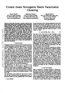
Fig. 2. Biclustering using a-NMF and a-PNMF based on the I-divergence for the synthetic data: (a) the original matrix, (b) the disordered or testing matrix. The biclustering results use (c) two-factor linear NMF, (d) BiOR-NM3F, (e) BiOR-NM3F-I and (f) Bi-QNMF.
600 800
600 800
1000
1000
1000
1000
1200
1200
1200
1200
1400 0
200
400 600 term
800
1400 0
200
400 600 term
800
1400 0
200
400 600 term
800
1400 0
200
400 600 term
800
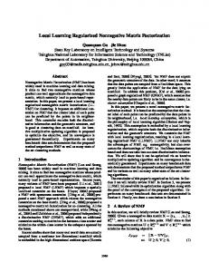
Fig. 3. Biclustering using (from left to right) two-factor linear NMF, BiOR-NM3F, BiOR-NM3F-I, and Bi-QNMF for the webkb data.
We ran each compared algorithm 10 times and picked the result with the smallest NMF approximation error. The resulting matrices are displayed in Fig. 2(c)–(f). It can be seen that the twofactor linear NMF method finds some but not all biclusters, especially the ones with a few rows. BiOR-NM3F performs even worse than the two-factor linear NMF, with the block sizes totally mismatched and many blocks containing dissimilar values. The failure of BiOR-NM3F could be caused by the wrong divergence type. We thus also compared the result by using BiOR-NM3F-I. However, the extended BiOR-NM3F generates identical columns in L and R, as well as a uniform S, which results in still disordered
visualization. Compared to the above methods, Bi-QNMF can well reconstruct all biclusters up to a block-wise permutation. Next, we compared the four methods on the real-world webkb dataset (see footnote 6). The data matrix contains a subset of the whole dataset, with two classes of 1433 documents and 933 terms. The ij-th entry of the matrix is the number of the j-th term that appears in the i-th document. Same as the tests on synthetic data, we reordered the matrix rows and columns by using the learned factorizing matrices of the compared methods. The resulting matrices are visualized in Fig. 3 using the Matlab command spy.
Z. Yang, E. Oja / Pattern Recognition 45 (2012) 1500–1510
The BiOR-NM3F method basically finds no biclusters. Only some small groups can barely be seen on the rightmost of the display. BiOR-NM3F-I is even worse, as there is no visually blockwise pattern in its result. The row cluster sizes found by the two-factor linear NMF and Bi-QNMF are roughly the same, about 650 rows for the first cluster and the rest for the second. However, linear NMF results in incoherent blocks, where the upper rows in the first row cluster are quite different from the others but very similar to the ones in the second row cluster. Such incoherence does not take place in the Bi-QNMF result, where the matrix is clearly divided into 2 � 2 biclusters. Suppose the input matrix is of size m � n. The computational cost of BiOR-NM3F, BiOR-NM3F-I and Bi-QNMF is Oðmn � max fr l ,r r gÞ per iteration, where rl and rr are the number of columns of L and R. For synthetic data, all NMF methods finish 20,000 iterations (converged) within 2 min. For the larger webkb dataset, the NMF biclustering algorithms converged within 2 h. 5.3. Estimating hidden Markov chains In a stationary Hidden Markov Chain Model (HMM), the observed output and the hidden state at time t are denoted by xðtÞ A f1, . . . ,ng and yðtÞ A f1, . . . ,rg, respectively. The joint probabilities of a consecutive pair are then given by X ij 9PðxðtÞ ¼ i,xðt þ1Þ ¼ jÞ and Y kl 9PðyðtÞ ¼ k,yðt þ 1Þ ¼ lÞ accordingly. For the noiseless model, we have X ¼ WYWT with W9PðxðtÞ ¼ i9yðtÞ ¼ kÞ. When noise is considered, this becomes an approximative QNMF problem X � WYWT . Particularly, when the approximation error is measured by squared Euclidean distance, the parameter estimation problem of HMM can be formulated as minimization of P JX�WYWT J2F over nonnegative W and Y and subject to i W ik ¼ 1 P for all k and kl Y kl ¼ 1. Previously, the above optimization problem has been difficult because the objective is quartic with respect to W. An earlier algorithm, named NNMF-HMM [35], interleaves minimizations over Y and one of the appearances of W, each of which is implemented by using matrix pseudo-inversion and truncation of negative entries. Now we have a much nicer algorithm for this QNMF problem. Using the presented deriving principle, we can obtain the multi� plicative update rule in the form of Eq. (10), where rW ¼ þ � T T T T T T T XWY þX WY, rW ¼ WYW WY þWY W WY, rY ¼ W XW, þ and rY ¼ WT WYWT W. We have compared the two methods on three datasets. The first is a synthetic sequence generated by using the procedure by x 10–3
synthetic
1507
Lakshminarayanan and Raich [35]. The other two are real-world datasets, one for letter sequence in the top 58 112 English words (see footnote 7) and the other for a genetic code sequence of homo sapiens (see footnote 8). The sizes of the observed input matrix are 22 � 22, 26 � 26, and 64 � 64, respectively. We empirically set the number of hidden states in all experiments. Both compared algorithms were run at least 10 000 iterations. The evolutions of HMM estimation objective are shown in Fig. 4. The new method is significantly more efficient than the old algorithm for all selected datasets. For the two smaller datasets, the objectives using NNMF-HMM tend to fluctuate a lot during the iterations, which is possibly caused by the brute-force truncation of negative entries. NNMF-HMM is more problematic for the largest dataset, where the approximation error only barely drops after thousands of epochs. By contrast, the objectives using QNMF-HMM decrease much faster and more stably. QNMF-HMM uses soft constraints during its learning. To verify that the constraint errors are trivial in the converged results, we P P P have checked the quantities k 91� i W ik 9 and 91� kl Y kl 9 as constraint error measures for W and Y, respectively. We repeated each experiment 100 times with different random initial guess of W and Y. The recorded means and standard deviations of the above constraint errors are shown in Table 2. We can see that the constraint errors are so small that they are negligible compared to the data dimensions. We also examined the final objectives using the compared methods. For QNMF-HMM, we normalized W in the end of learning to force the strict constraints. The normalization actually causes little loss because of the negligible constraint errors. The error bars of the final objectives are illustrated in Fig. 5, from which we can see that the new method can achieve much smaller approximation errors than the old one. In addition, the variations of QNMF-HMM results are very small, which indicates the our method is pretty robust. The squared Euclidean distance in the HMM estimation can be replaced with the Kullback–Leibler divergence, which is a more canonical difference measure for probabilities. With such divergence we can reveal some interesting structure in the fitted Table 2 Constraint errors of factorizing matrices (W and Y) using QNMF-HMM.
W Y
Synthetic
English words
Genetic codes
8.9e � 067 3.8e � 05 1.7e � 087 1.2e � 07
3.3e � 057 3.5e � 05 2.2e � 077 5.6e � 07
6.1e � 06 7 6.1e� 06 2.7e � 07 7 2.2e� 07
English words
x 10–3
8
5.5 5
3.5
7
3
4.5 objective
objective
3.5 3 2.5
objective
6
4
genetic codes
x 10–4
5 4
2.5 2 1.5
2
3 1
1.5 2
1
0.5 10–2
10–1
100
time (seconds)
101
10
–3
10
–2
10
–1
10
0
10
1
time (seconds) Fig. 4. Evolutions of the HMM estimation objective.
10–2
100 time (seconds)
102
1508
Z. Yang, E. Oja / Pattern Recognition 45 (2012) 1500–1510
converged objective (log–scale)
100
10–1
10–2
10–3
10–4 NNMF–HMM QNMF–HMM
10–5
synthetic
English words
genetic codes
Fig. 5. HMM estimation objectives for the selected datasets.
If the graph and its permutation are represented by (weighted) adjacency matrices, denoted by A and B, the isomorphism can be written as B ¼ PAPT , where P is a permutation matrix. The computation time of existing combinatorial algorithms to find the exact correct permutation grows exponentially as the number of nodes increases. For large graphs, approximation is therefore needed. A classical approximation algorithm by Umeyama [36] uses eigendecomposition and simply forces nonnegativity by using absolute values of the eigenvectors. Ding et al. [18] pointed out that the results of Umeyama’s algorithm are not satisfactory, and proposed a special case of QNMF formulation based on the Euclidean distances: to minimize JB�WAWT J2F subject to WT W ¼ I and WZ 0. After the multiplicative updates have converged, the permutation P is obtained by using the classical Hungarian algorithm on elementwise inverse of WT [37]. This method, abbreviated by EU-QNMF, was reported to be superior to Umeyama’s algorithm on dense graphs generated as follows: Aij ¼ 100r ij and Bij ¼ ðPt APTt Þij ð1 þ Esij Þ, where rij and sij are uniform random numbers in [0, 1], Pt is a permutation and E sets the noise level. However, many real-world networks are not generated like this. They should be sparse and thus the Gaussian assumption that underlies the Euclidean-NMF does not hold. We are thus motivated to use the I-divergence, i.e. to minimize DI ðBJWAWT Þ over WZ 0 and subject to WT W ¼ I. This corresponds to underlying Poisson distribution which is more suitable for sparse occurrences. We abbreviate the new method by I-QNMF. The comparison results of EU-QNMF and I-QNMF for graph matching are shown in Tables 3 and 4 for directed and undirected graphs, respectively. All graphs in use are binary-valued. Most graphs were downloaded from the University of Florida Sparse Matrix Collection (see footnote 9). Some others were taken from Newman’s network data collection (see footnote 3) and from the Pajek datasets (see footnote 4). For fair comparison, we used a neutral quantity to measure the matching error, which is defined Table 3 Errors (mean 7 standard deviation) in directed graph matching. Graph
Size
EU-QNMF
I-QNMF
SAMPIN WOLFK football35 cage5 BKOFFC curtis54 will57 PRISON CAG_mat72 GlossGT
18 20 35 37 40 54 57 67 72 72
1.20 70.38 1.807 0.30 7.207 2.28 9.207 1.03 0.007 0.00 96.40 7 5.38 87.60 7 3.24 4.407 0.45 0.207 0.06 4.607 0.67
0.00 70.00 2.10 7 0.07 8.20 7 0.81 12.80 7 0.53 0.00 70.00 56.60 7 2.63 35.80 7 1.36 6.70 7 0.37 0.00 70.00 4.80 7 0.19
Fig. 6. Reordered joint probability matrix by the letter clusters.
model of the English words data. Here we only focus on the QNMFHMM algorithm because there is no existing implementation or straightforward extension of NNMF-HMM for Kullback–Leibler divergence. The latent or blockwise structure of the joint probability matrix X is visualized in Fig. 6 by reordering the rows and columns according to the letter clusters, where lighter dots correspond to larger values. Each English letter was assigned to one of six clusters according to largest entries in the learned W rows. In this way we can group the letters into the following six groups: (1) D, Q, R, S, X, (2) C, G, (3) B, F, H, J, K, L, M, P, T, V, W, Z, (4) N, (5) A, I, O, U, and (6) E, Y. The first four groups are consonants, while the remaining two are basically vowels. A plausible interpretation of such division is that English words consist of syllables where a consonant is often followed by a vowel and vice versa. The letter N itself forms a group probably because we used a pretty large list of English words where suffixes such as ING and TION occur frequently. 5.4. Graph matching Given a graph and its node-permuted version, the graph matching problem is to find the correspondence of graph nodes.
Table 4 Errors (mean 7 standard deviation) in undirected graph matching. Graph
Size
EU-QNMF
I-QNMF
RDPOS PADGB PADGM WOLFN strike ZACHC ZACHE korea1 korea2 mexican_power Sawmill dolphins
14 16 16 20 24 34 34 35 35 35 36 62
4.80 70.41 9.207 0.98 5.607 0.66 3.20 70.59 25.60 7 1.36 43.20 7 4.76 27.60 7 2.97 39.20 7 2.72 29.60 7 1.78 20.007 5.25 70.40 72.14 137.80 7 8.31
4.20 70.27 10.20 7 0.64 6.20 7 0.40 2.00 70.34 12.20 7 1.02 10.40 7 0.08 5.00 70.36 12.40 7 0.82 12.80 7 0.50 10.80 7 0.62 16.00 7 0.69 31.20 7 1.17
Z. Yang, E. Oja / Pattern Recognition 45 (2012) 1500–1510
as #fXORðPAPT ,BÞg, i.e. the number of different edges between the estimated permuted matrix and the true permuted matrix. A smaller error indicates better matching quality. In summary, I-QNMF performs almost at the same level as EU-QNMF for small or easy-matched graphs. However, the former is significantly better for larger and more difficult graphs in terms of both smaller mean errors and smaller deviations. This advantage is even clearer for undirected graphs. The computational cost of both NMF graph matching algorithms is OðN3 Þ for a graph with N nodes. For small graphs such as SAMPIN and strike, the algorithms can finish 20,000 iterations (converged) within a few seconds. For larger graphs such as GlossGT and dolphins, the algorithms converged within about 10 min.
6. Conclusions We have formulated the general problem of approximative quadratic nonnegative matrix factorization and proposed a framework to develop multiplicative optimization algorithms that are guaranteed to decrease the objective function. Multiplicative algorithms for two typical QNMF factorization forms based on a great variety of approximation error measures, as well as the stochasticity and orthogonality constraints, were presented. The proposed method has been applied to four different pattern recognition problems, where QNMF is shown to be more advantageous than other state-of-the-art NMF methods. Our work opens the door to higher-order nonnegative matrix factorizations, but this is definitely not the end of this stream of research. For optimization, recently some faster additive methods for fast optimization of NMF objectives have been developed (e.g. [38,39,5]). However, the speedup is achieved for only limited kinds of divergences, especially the squared Euclidean distance where the Hessian has a particularly simple form. Otherwise, these additive approaches could be sensitive to the choice of extra parameters such as learning rate or line search step. How to extend these methods to many other divergences remains an open problem. Alternatively, we could implant efficient approximative second-order optimization techniques into the multiplicative updates for faster convergence. In addition, scalable QNMF algorithms for more divergence types other than squared Euclidean distance could be developed using advanced streaming or distributed computation techniques. Moreover, we have found that many QNMF multiplicative algorithms converge to similar local minima up to a certain component order. The theoretical analysis of the global minimum up to certain permutations needs further investigation. Besides matrix products, the factorized approximation may involve nonlinear operators, for example, a nonlinear activation function that interleaves a factorizing matrix and its transpose. This kind of approximation could be extended to the field of nonnegative neural networks and connected to the deep learning principle when multiple such groups of elements are stacked.
Appendix A. Proof of Theorem 2 Decompose k into two nonnegative parts: k ¼ k þ �k� , where � ¼ ð9lk 9 þ lk Þ=2 and lk ¼ ð9lk 9�lk Þ=2. We can then write the ~ ik Þ� ~ kÞ ¼ J ðWÞ ~ þ P l þ ð1�P W augmented objective as LðW, k k i P ~ P � k lk ð1� i W ik Þ. Next, we apply the original upper-bounding P þ P ~ P � ~ ~ ~ kÞ rGðW,WÞ þ k lk ð1� i W on J ðWÞ: LðW, ik Þ� k lk P ~ ð1� i W ik Þ. Combining individual upper-bounds into two, we
lkþ
obtain the ultimate auxiliary function ! ~ ik u þ X W ik W X W ik � ~ ~ GðW,WÞ ¼ ðrik þ lk Þ� u W v ik ik ik
1509
~ ik W W ik
!v �
þ
ðrik þ lk Þ,
up to an additive constant, where u ¼ maxðcmax ,1Þ and ~ W ~ ik ¼ 0 leads to v ¼ minðcmin ,1Þ. Setting @G=@ " #s r�ik þ lkþ W new ¼ W ik ðA:1Þ ik rikþ þ l�k ~ kÞ=@W ~ ik ¼ 0, we get ðr þ �r� Þ � with s ¼ 1=ðu�vÞ. From @LðW, ik P lk ¼ 0. By multiplying both sides with i W ik and making use of P P the fact @LðW, kÞ=@lk ¼ 0, i.e. i W ik ¼ 1, we obtain lk ¼ i W ik þ P � rik � i W ik rik . Inserting this to Eq. (A.1), the multiplicative update rule becomes Eq. (10).
Appendix B. Proof of Theorem 3 and Corollary 4 Similar to the proof of Theorem 2, we decompose K into two nonnegative parts: K ¼ K þ �K� . We can then construct the auxiliary function of the generalized objective ~ KÞ ¼ J ðWÞ�Trð ~ LðW, K þ WT WÞ þ TrðK� WT WÞ þconstant ! ~ W ~ X þ W ~ Lkl W ik W il 1þ ln ik il rJ ðWÞ� W ik W il ikl ~ 2 X ðWK� Þ W ik ik þconstant W ik ik ! ~ ik u þ X W ik W r ðr þ 2WK� Þik u W ik ik ! ~ ik v � X W ik W ~ W ~ ,WÞ, � ðr þ2WK þ Þik þ constant9Gð v W ik ik þ
~ W ~ ik ¼ 0 where u ¼ maxðcmax ,2Þ and v ¼ minðcmin ,0Þ. Setting @G=@ gives � � �s ðr þ 2WK þ Þik W new ¼ W ik ðB:1Þ ik þ � ðr þ 2WK Þik þ
�
with s ¼ 1=ðu�vÞ. From @LðW, KÞ=@W ¼ 0, we get 2WK ¼ r �r . Using @LðW, KÞ=@K ¼ 0, i.e. WT W ¼ I, one obtains K ¼ 12 WT þ � ðr �r Þ: Inserting this to (B.1), the multiplicative update rule becomes Eq. (11). The proof of Corollary 4 is similar to that of the theorem, except that we replace the bound of �TrðK þ WT WÞ with a hyperP ~ þ plane �2 ikl W il Llk þ constant. The corollary thus results in a larger exponential or step size s than Theorem 3. References [1] D.D. Lee, H.S. Seung, Learning the parts of objects by non-negative matrix factorization, Nature 401 (1999) 788–791. [2] D.D. Lee, H.S. Seung, Algorithms for non-negative matrix factorization, Advances in Neural Information Processing Systems 13 (2001) 556–562. [3] P.O. Hoyer, Non-negative matrix factorization with sparseness constraints, Journal of Machine Learning Research 5 (2004) 1457–1469. [4] S. Choi, Algorithms for orthogonal nonnegative matrix factorization, in: Proceedings of IEEE International Joint Conference on Neural Networks, 2008, pp. 1828–1832. [5] D. Kim, S. Sra, I.S. Dhillon, Fast projection-based methods for the least squares nonnegative matrix approximation problem, Statistical Analysis and Data Mining 1 (1) (2008) 38–51. [6] C. Fe´votte, N. Bertin, J.-L. Durrieu, Nonnegative matrix factorization with the Itakura–Saito divergence: with application to music analysis, Neural Computation 21 (3) (2009) 793–830. [7] S. Behnke, Discovering hierarchical speech features using convolutional nonnegative matrix factorization. in: Proceedings of IEEE International Joint Conference on Neural Networks, vol. 4, 2003, pp. 2758–2763.
1510
Z. Yang, E. Oja / Pattern Recognition 45 (2012) 1500–1510
[8] H. Kim, H. Park, Sparse non-negative matrix factorizations via alternating non-negativity-constrained least squares for microarray data analysis, Bioinformatics 23 (12) (2007) 1495–1502. [9] A. Cichocki, R. Zdunek, Multilayer nonnegative matrix factorization using projected gradient approaches, International Journal of Neural Systems 17 (6) (2007) 431–446. [10] C. Ding, T. Li, W. Peng, On the equivalence between non-negative matrix factorization and probabilistic latent semantic indexing, Computational Statistics and Data Analysis 52 (8) (2008) 3913–3927. [11] A. Cichocki, R. Zdunek, A.-H. Phan, S. Amari, Nonnegative Matrix and Tensor Factorizations: Applications to Exploratory Multi-Way Data Analysis, John Wiley, 2009. [12] R. Kompass, A generalized divergence measure for nonnegative matrix factorization, Neural Computation 19 (3) (2006) 780–791. [13] I.S. Dhillon, S. Sra, Generalized nonnegative matrix approximations with Bregman divergences. in: Advances in Neural Information Processing Systems, vol. 18, 2006, pp. 283–290. [14] A. Cichocki, H. Lee, Y.-D. Kim, S. Choi, Non-negative matrix factorization with a-divergence, Pattern Recognition Letters 29 (2008) 1433–1440. [15] A. Pascual-Montano, J.M. Carazo, K. Kochi, D. Lehmann, R.D. Pascual-Marqui, Nonsmooth nonnegative matrix factorization (nsNMF), IEEE Transactions on Pattern Analysis and Machine Intelligence 28 (3) (2006) 403–415. [16] C. Ding, T. Li, W. Peng, H. Park, Orthogonal nonnegative matrix T-factorizations for clustering, in: Proceedings of the 12th ACM SIGKDD International Conference on Knowledge Discovery and Data Mining, 2006, pp. 126–135. [17] C. Ding, T. Li, M.I. Jordan, Convex and semi-nonnegative matrix factorizations, IEEE Transactions on Pattern Analysis and Machine Intelligence 32 (1) (2010) 45–55. [18] C. Ding, T. Li, M.I. Jordan, Nonnegative matrix factorization for combinatorial optimization: spectral clustering, graph matching, and clique finding, in: Proceedings of the 8th IEEE International Conference on Data Mining (ICDM), 2008, pp. 183–192. [19] C. Ding, X. He, K-means clustering via principal component analysis, in: Proceedings of International Conference on Machine Learning (ICML), 2004, pp. 225–232. [20] Z. Yang, E. Oja, Linear and nonlinear projective nonnegative matrix factorization, IEEE Transaction on Neural Networks 21 (5) (2010) 734–749. [21] Z. Yuan, E. Oja, Projective nonnegative matrix factorization for image compression and feature extraction, in: Proceedings of 14th Scandinavian Conference on Image Analysis (SCIA), Joensuu, Finland, 2005, pp. 333–342. [22] Z. Yang, E. Oja, Unified development of multiplicative algorithms for linear and quadratic nonnegative matrix factorization, IEEE Transactions on Neural Networks, doi:org/10.1109/TNN.2011.2170094, in press.
[23] B. Long, Z. Zhang, P.S. Yu, Coclustering by block value decomposition, in: Proceedings of the Eleventh ACM SIGKDD International Conference on Knowledge Discovery in Data Mining, 2005, pp. 635–640. [24] W. Liu, N. Zheng, X. Lu, Non-negative matrix factorization for visual coding. in: Proceedings of IEEE International Conference on Acoustics, Speech, and Signal Processing (ICASSP), vol. 3, 2003, pp. 293–296. [25] Z. Yang, J. Laaksonen, Multiplicative updates for non-negative projections, Neurocomputing 71 (1–3) (2007) 363–373. [26] J. Yoo, S. Choi, Orthogonal nonnegative matrix factorization: multiplicative updates on Stiefel manifolds, in: Proceedings of the 9th International Conference on Intelligent Data Engineering and Automated Learning, 2008, pp. 140–147. [27] Z. Yang, Z. Yuan, J. Laaksonen, Projective non-negative matrix factorization with applications to facial image processing, International Journal on Pattern Recognition and Artificial Intelligence 21 (8) (2007) 1353–1362. [28] E.M. Airoldi, D.M. Blei, S.E. Fienberg, E.P. Xing, Mixed membership stochastic blockmodels, Journal of Machine Learning Research 9 (2008) 1981–2014. [29] Z. Yang, E. Oja, Online projective nonnegative matrix factorization for large datasets, in: NIPS Workshop on Low-Rank Methods for Large-Scale Machine Learning, 2010. [30] J. Shi, J. Malik, Normalized cuts and image segmentation, IEEE Transactions on Pattern Analysis and Machine Intelligence 22 (8) (2000) 888–905. [31] S.X. Yu, J. Shi, Multiclass spectral clustering. in: Proceedings of the 9th IEEE International Conference on Computer Vision, vol. 2, 2003, pp. 313–319. [32] X. Zhu, Z. Ghahramani, J. Lafferty, Semi-supervised learning using gaussian fields and harmonic functions, in: Proceedings of the 20th International Conference on Machine Learning (ICML), 2003, pp. 912–919. [33] L. Grady, Random walks for image segmentation, IEEE Transactions on Pattern Analysis and Machine Intelligence 28 (11) (2006) 1768–1783. [34] L. van der Maaten, G. Hinton, Visualizing data using T-SNE, Journal of Machine Learning Research 9 (2008) 2579–2605. [35] B. Lakshminarayanan, R. Raich, Non-negative matrix factorization for parameter estimation in hidden Markov models, in: Proceedings of IEEE International Workshop on Machine Learning For Signal Processing, 2010, pp. 89–94. [36] S. Umeyama, An eigendecomposition approach to weighted graph matching problems, IEEE Transactions on Pattern Analysis and Machine Intelligence 10 (5) (1988) 695–703. [37] H.W. Kuhn, The Hungarian method for the assignment problem, Naval Research Logistics Quarterly 2 (1955) 83–97. [38] C.-J. Lin, Projected gradient methods for non-negative matrix factorization, Neural Computation 19 (2007) 2756–2779. [39] R. Zdunek, A. Cichocki, Nonnegative matrix factorization with quadratic programming, Neurocomputing 71 (10–12) (2008) 2309–2320.
Zhirong Yang received his Bachelor and Master degrees from Sun Yat-Sen University, China in 1999 and 2002, and Doctoral degree from Helsinki University of Technology, Finland in 2008, respectively. Presently he is a postdoctoral researcher with the Department of Information and Computer Science at Aalto University. His current research interests include pattern recognition, machine learning, computer vision, and information retrieval, particularly focus on nonnegative learning, information visualization, optimization, discriminative feature extraction and visual recognition. He is a member of the Institute of Electrical and Electronics Engineers (IEEE) and the International Neural Network Society (INNS).
Erkki Oja received the D.Sc. degree from Helsinki University of Technology in 1977. He is a Director of the Adaptive Informatics Research Centre and Professor at the Department of Information and Computer Science, Aalto University (former Helsinki University of Technology), Finland. He serves as the Chairman of the Finnish Research Council for Natural Sciences and Engineering. He holds an honorary doctorate from Uppsala University, Sweden, and from two Finnish universities. He has been a research associate at Brown University, Providence, RI, and a visiting professor at the Tokyo Institute of Technology and the Universite Pantheon-Sorbonne, Paris. He is the author or coauthor of more than 300 articles and book chapters on pattern recognition, computer vision, and neural computing, and three books: ‘‘Subspace Methods of Pattern Recognition’’ (New York: Research Studies Press and Wiley, 1983), which has been translated into Chinese and Japanese; ‘‘Kohonen Maps’’ (Amsterdam, The Netherlands: Elsevier, 1999), and ‘‘Independent Component Analysis’’ (New York: Wiley, 2001; also translated into Chinese and Japanese). His research interests are in the study of principal component and independent component analysis, self-organization, statistical pattern recognition, and applying artificial neural networks and machine learning to computer vision and signal processing. Oja is a member of the Finnish Academy of Sciences, Fellow of the Institute of Electrical and Electronics Engineers (IEEE), Founding Fellow of the International Association of Pattern Recognition (IAPR), Past President of the European Neural Network Society (ENNS), and Fellow of the International Neural Network Society (INNS). He is a member of the editorial boards of several journals and has been in the program committees of several recent conferences. He was general chair of the 2010 IEEE International Workshop on Machine Learning for Signal Processing (MLSP) and the 2011 International Conference on Artificial Neural Networks (ICANN). Prof. Oja is the recipient of the 2004 IAPR Pierre Devijver Award, the 2006 IEEE Computational Intelligence Society Neural Networks Pioneer Award, and the 2010 INNS Hebb Award.