Mar 8, 2006 - as a linear combination of function and derivative values of f at the ...... arctan. ( κ1 κ2. + ε. )} ,. Ωε,1. = {. (x, y) : x2 + y2 < 1, y> 0, arctan. ( κ1 κ2.
MATHEMATICS OF COMPUTATION Volume 75, Number 255, July 2006, Pages 1233–1258 S 0025-5718(06)01854-0 Article electronically published on March 8, 2006
QUADRATURE METHODS FOR MULTIVARIATE HIGHLY OSCILLATORY INTEGRALS USING DERIVATIVES ARIEH ISERLES AND SYVERT P. NØRSETT We dedicate this paper to the memory of Germund Dahlquist
Abstract. While there exist effective methods for univariate highly oscillatory quadrature, this is not the case in a multivariate setting. In this paper we embark on a project, extending univariate theory to more variables. Inter alia, we demonstrate that, in the absence of critical points and subject to a nonresonance condition, an integral over a simplex can be expanded asymptotically using only function values and derivatives at the vertices, a direct counterpart of the univariate case. This provides a convenient avenue towards the generalization of asymptotic and Filon-type methods, as formerly introduced by the authors in a single dimension, to simplices and, more generally, to polytopes. The nonresonance condition is bound to be violated once the boundary of the domain of integration is smooth: in effect, its violation is equivalent to the presence of stationary points in a single dimension. We further explore this issue and propose a technique that often can be used in this situation. Yet, much remains to be done to understand more comprehensively the influence of resonance on the asymptotics of highly oscillatory integrals.
1. Introduction Let Ω ⊂ Rd be a connected, open, bounded domain with sufficiently smooth boundary. We are concerned in this paper with the computation of the highly oscillatory integral � (1.1) I[f, Ω] = f (x)eiωg(x) dV, Ω
where f, g : R → R are smooth, g �≡ 0, dV is the volume differential and ω � 1. Integrals of this form feature frequently in applications, not least in applications of the boundary element method to problems originating in electromagnetics and in acoustics [STW90]. Another important source of highly oscillatory integrals is geometric numerical integration and methods for highly oscillatory differential equations that expand the solution in multivariate integrals [DS03, Ise02, Ise04a]. Building upon earlier work in [Ise04b, Ise05], we have recently developed two general methods for the integration of univariate highly oscillatory integrals using just a small number of function values and derivatives at the endpoints and at the stationary points of g [IN05a, IN05b]. The outstanding feature of these methods, which they share with an earlier method of Levin [Lev96], is that their precision d
Received by the editor February 17, 2005 and, in revised form, July 28, 2005. 2000 Mathematics Subject Classification. Primary 65D32; Secondary 41A60, 41A63. c �2006 American Mathematical Society Reverts to public domain 28 years from publication
1233
1234
ARIEH ISERLES AND S. P. NØRSETT
grows with increasing oscillation. Indeed, judiciously using derivatives, it is possible to speed up the decay of the error arbitrarily fast for large ω. The purpose of this paper is to extend this work into the realm of multivariate integrals of the form (1.1). To this end we provide in Section 2 a brief overview of the univariate theory and of the asymptotic and Filon-type methods. In Section 3 we commence the main numerical part of this paper by examining product rules for integration in parallelepipeds. Although results of this section can be alternatively obtained by techniques introduced later in the paper, there are valid reasons to examine product rules first, since they represent the most obvious extension of univariate theory, while demonstrating difficulties peculiar to multivariate quadrature. Our point of departure in Section 4 is a d-dimensional regular simplex Sd with vertices at the origin and at the unit vectors e1 , e2 , . . . , ed ∈ Rd , combined with a linear oscillator. We demonstrate how, subject to a nonresonance condition, it is possible to represent highly oscillatory integration in Sd in terms of surface integrals across its d + 1 faces, themselves (d − 1)-dimensional simplices. Iterating this procedure ultimately leads to an asymptotic expression of the integral I[f, Sd ] as a linear combination of function and derivative values of f at the vertices of Sd . This allows for a straightforward generalization of univariate highly oscillatory quadrature methods to this setting. The theme of Section 4 is continued in Section 5, except that there we allow more general, nonlinear oscillators. This requires a more elaborate nonresonance condition and more subtle analysis. In Section 6 we develop a Stokes-type formula, which allows us, subject to nonresonance conditions, to express a highly oscillatory integral in Sd as an asymptotic expansion on its boundary. As well as providing an alternative tool for the analysis of Section 5, this expansion is interesting in its own sake. Finally, in Section 7 we consider multivariate highly oscillatory quadrature in polytopes. Each polytope can be tiled by simplices, and this tessellation allows us to infer from earlier material in this paper to general (neither necessarily convex, nor even simply connected) polytopes. Thus, subject to nonresonance, we express a highly oscillatory integral over a polytope asymptotically as a sum of function and derivative values at its vertices. The outcome are two general quadrature techniques, the asymptotic method and the Filon-type method. A multivariate domain with smooth boundary can be approximated by polytopes, hence it might be tempting to use the dominated convergence theorem and generalize our results from polytopes to such domains. Unfortunately, the nonresonance condition breaks down once we consider smooth boundaries. We explore these issues further, identify this breakdown with lower-dimensional stationary points and present a technique, a combination of an asymptotic expansion and a Filon-type method, which can be used in a bivariate setting. A major issue in univariate computation of highly oscillatory integrals is possible presence of stationary points, where the derivative of oscillator g vanishes [Olv74, Ste93]. In that instance the integral cannot be expanded asymptotically in integer negative powers of ω. The expansion employs fractional powers of ω and is considerably more complicated. The standard means of analysis is the method of stationary phase [Olv74], except that it is insufficient for our needs. A considerably simpler, yet more suitable from our standpoint, alternative is a technique originally
MULTIVARIATE HIGHLY OSCILLATORY QUADRATURE
1235
introduced in [IN05a]. The same distinction is crucial in a multivariate setting. As long as ∇g �= 0 in the closure of Ω, we can expand I[f, Ω] in negative integer powers of ω and exploit this asymptotic expansion in construction of numerical methods. However, once we allow nondegenerate critical points ξ ∈ Ω where ∇g(ξ) = 0, det ∇∇� g(ξ) �= 0, the situation is considerably more complex [Ste93]. In this paper we do not pursue this issue, since critical points are explicitly excluded from our setting by the nonresonance condition. Having said this, as we have already mentioned, breakdown of nonresonance for smooth boundaries is equivalent to the presence of univariate stationary points. Thus, even if we require that ∇g(x) �= 0 in the closure of Ω, problems associated with the presence of stationary points are generic to domains with smooth boundaries. Our present understanding of univariate quadrature methods for oscillators with stationary points is unequal to this task and calls for further research. 2. The univariate case Let d = 1 and Ω = (a, b). In other words, we consider � b f (x)eiωg(x) dx. (2.1) I[f, (a, b)] = a
Let us first consider strictly monotone oscillators g. In that case it has been proved in [IN05a] that for any f ∈ C∞ [a, b] the integral in (2.1) admits the asymptotic expansion (2.2) � � iωg(b) ∞ � e 1 eiωg(a) σm [f ](b) − � σm [f ](a) , ω � 1, I[f, (a, b)] ∼ − (−iω)m+1 g � (b) g (a) m=0 where σ0 [f ](x) σm [f ](x)
= f (x), d σm−1 [f ](x) , = dx g � (x)
m = 1, 2, . . . .
Note that each σm [f ] is a linear combination of f (i) , i = 0, 1, . . . , m, with coefficients that depend upon g and its derivatives. Truncating (2.2) results in the asymptotic method � � iωg(b) s−1 � e 1 eiωg(a) σ σ [f, (a, b)] = − [f ](b) − [f ](a) , (2.3) QA m m s (−iω)m+1 g � (b) g � (a) m=0 and it follows immediately that
� −s−1 � QA . s [f, (a, b)] − I[f, (a, b)] ∼ O ω
The information required to attain this rate of asymptotic decay, which improves as the frequency ω grows, is just the values of f, f � , . . . , f (s−1) at the endpoints of the interval. An alternative to the asymptotic method (2.3) which, while requiring identical information and producing the same rate of asymptotic decay, is typically more accurate is the Filon-type method. [IN05a]. In its basic reincarnation we construct a
1236
ARIEH ISERLES AND S. P. NØRSETT
degree-(2s−1) Hermite interpolating polynomial ψ, say, such that ψ (j) (a) = f (j) (a), ψ (j) (b) = f (j) (b), j = 0, 1, . . . , s − 1, and set QF s [f, (a, b)] = I[ψ, (a, b)].
(2.4)
It readily follows, applying (2.2) to ψ − f , that
� −s−1 � , QF s [f, (a, b)] − I[f, (a, b)] = I[ψ − f, (a, b)] = O ω
ω � 1.
The Filon-type method can be enhanced by interpolating f not just at a and b but also at intermediate points. Although the asymptotic rate of decay remains the same, the size of the error is significantly reduced. We refer to [IN05a] for details and examples and to [IN05b] for techniques to estimate the error and an explanation why Filon is usually (but not always) likely to produce a smaller error than the asymptotic method. A potential drawback of Filon-type methods is the need to evaluate explicitly the moments � b
xm eiωg(x) dx
µm (ω) = a
of the oscillator g for a suitable range of nonnegative integers m. Although straightforward for quadratic g, this represents a genuine limitation of Filon-type methods. This is the place to mention in passing the recent alternative approach of Levin-type methods, which does not require the knowledge of moments [Olv05]. Unfortunately, Levin-type methods cannot cater for stationary points: as often in computational mathematics, no method is superior in all its aspects. Both (2.3) and (2.4) can be generalized to cater for oscillators g with stationary points in (a, b). For example, suppose that g � (y) = 0, g �� (y) �= 0 for some y ∈ (a, b) and g � (x) �= 0 for x ∈ [a, b]\{y}. In that case the asymptotic expansion of I[f, (a, b)] does not depend any longer just on f and its derivatives at the endpoints. Then (2.2) needs to be replaced by the asymptotic expansion ∞ �
1 ρ [f ](y) m m (−iω) m=0 � iωg(b) ∞ � e 1 {ρm [f ](b) − ρm [f ](y)} − m+1 (−iω) g � (b) m=0
I[f, (a, b)] ∼ µ0 (ω) (2.5)
� eiωg(a) {ρm [f ](a) − ρm [f ](y)} , − � g (a)
ω � 1,
where µ0 (ω) is the zeroth moment of the oscillator g and ρ0 [f ](x) ρm [f ](x)
= f (x), d ρm−1 [f ](x) − ρm−1 [f ](y) , = dx g � (x)
m = 1, 2, . . . .
Note that ρm for m ≥ 1 has a removable singularity at y, but, as long as f is smooth in [a, b], so is each ρm However, while each ρm depends on f, f � , . . . , f (m) at the endpoints a and b, it also depends on f, f � , . . . , f (2m) at the stationary point ξ [IN05a]. The expansion (2.5) can be easily generalized to stationary points of degree r, i.e., when g � (y) = · · · = g (r) (y) = 0, g (r+1) (y) �= 0, to several stationary points in (a, b) and to stationary points at the endpoints.
MULTIVARIATE HIGHLY OSCILLATORY QUADRATURE
1237
Once the expansion (2.5) is truncated, we obtain for every s ≥ 1 the asymptotic method s−1 � 1 [f ] = µ (ω) ρm [f ](y) QA 0 s (−iω)m m=0 � iωg(b) s−1 � e 1 (2.6) {ρm [f ](b) − ρm [f ](y)} − m+1 (−iω) g � (b) m=0 � eiωg(a) − � {ρm [f ](a) − ρm [f ](y)} , g (a) 1
a generalization of (2.3) to the present setting. Since µ0 (ω) ∼ O ω − 2 [Ste93], we can prove that
−s− 12 , ω � 1. QA s [f ] − I[f, (a, b)] = O ω (i) Observe that QA (a), f (i) (b), i = 0, 1, . . . , s − 1, but also on s [f ] depends on f (i) f (y), i = 0, 1, . . . , 2s − 2. The Filon-type approach can be generalized to the present setting in a natural way. Specifically, we choose nodes c1 = a < c2 < · · · < cν−1 < cν = b such that , . . . , cν−1 } and multiplicities m1 , m2 , . . . , mν ∈ Z. Let ψ be a polynomial y ∈ {c2 , c3� of degree ml − 1 which interpolates f and its derivatives at the nodes,
ψ (i) (ck ) = f (i) (ck ),
i = 0, . . . , mk − 1,
k = 1, . . . , ν.
The Filon-type method is given, again, by (2.4). Note that n1 , nν ≥ s and mr ≥ −s− 12 for ω � 1. Thus, 2s − 1, where cr = y, imply that QF s [f ] − I[f, (a, b)] = O ω we again replicate the asymptotic order of decay of the asymptotic method, use the same information, but have access to extra degrees of freedom that typically allow for higher precision. 3. Product rules The simplest generalization of univariate quadrature to multivariate setting is by using product rules, and it is applicable to the case when Ω ⊂ Rd is a parallelepiped. Although we will consider many more general domains later in the paper, it is useful to commence with a simple example since it illustrates many issues that will be at the center of our attention. Without loss of generality we may assume that Ω is a unit cube. We consider just the case d = 2, but general dimensions can be treated by identical means at the price of more elaborate algebra. Thus, we wish first to expand asymptotically and subsequently to approximate the integral � b� b f (x, y)eiωg(x,y) dydx, (3.1) I[f, (a, b)2 ] = a
a
where f and g are smooth functions and g is real. We assume that the oscillator g is separable, x, y ∈ [a, b], g(x, y) = g1 (x) + g2 (y), and that (3.2)
g1� (x), g2� (y) �= 0,
x, y ∈ [a, b].
1238
ARIEH ISERLES AND S. P. NØRSETT
The separability condition is stronger than absolutely necessary and will be relaxed later in the paper, but it renders the algebra considerably simpler and, for the time being, will suffice to illustrate salient points of our analysis. We commence by expanding the inner integral in (3.1) into asymptotic series (2.2), a procedure justified by the assumptions (3.2). Thus, exchanging integration and summation, � b � iωg(x,b) ∞ � e 1 σ0,m2 [f ](x, b) I[f, (a, b)2 ] ∼ − m2 +1 (−iω) g2� (b) a m2 =0 � eiωg(x,a) − � σ0,m2 [f ](x, a) dx, g2 (a) where σ0,0 [f ] = f,
σ0,m2 [f ] =
∂ σ0,m2 −1 [f ] , ∂y g2�
m2 ≥ 1.
Next, we expand the remaining integral in asymptotic series (2.2) and rearrange terms, � iωg(b,b) ∞ ∞ � � e 1 σm ,m [f ](b, b) I[f, (a, b)2 ] ∼ � m +m +2 1 2 (−iω) g1 (b)g2� (b) 1 2 m =0 m =0 1
−
e
eiωg(a,a)
σm ,m [f ](b, a) + g1� (b)g2� (a) 1 2 � iωg(a,b)
σm ,m [f ](a, a) g1� (a)g2� (a) 1 2
e σm ,m [f ](a, b) g1� (a)g2� (b) 1 2 m � ∞ � � eiωg(b,b) 1 −
(3.3)
2
iωg(b,a)
=
m=0
− −
(−iω)m+2
k=0
g1� (b)g2� (b)
σk,m−k [f ](b, b)
eiωg(b,a)
σk,m−k [f ](b, a) + g1� (b)g2� (a) � iωg(a,b)
eiωg(a,a)
σk,m−k [f ](a, a) g1� (a)g2� (a)
e σk,m−k [f ](a, b) , g1� (a)g2� (b)
where σm1 ,m2 [f ] =
∂ σm1 −1,m2 [f ] , ∂x g1�
m1 ≥ 1.
Let h ∈ C[(a, b)2 ] and ∂1 [h] =
∂ h , ∂x g1�
∂2 [h] =
∂ h . ∂y g2�
Separability of g implies that ∂1 ∂2 [h] =
1 g1� g2�
g �� ∂h g �� ∂h g �� g �� ∂2h − � 2� 2 − � 21 � + � 12 2� 2 h = ∂2 ∂1 [h]. ∂x∂y g1 g2 ∂x g1 g2 ∂y g1 g2
Therefore the two operators commute, and we can redefine the function σm1 ,m2 , σm1 ,m2 [f ] = ∂1m1 ∂2m2 [f ], where ∂1 and ∂2 can be applied in any order.
m1 , m2 ≥ 0,
MULTIVARIATE HIGHLY OSCILLATORY QUADRATURE
1239
A number of observations are in order. As will be evident later in the paper, they reflect a more general state of affairs and illustrate how the univariate theory of [IN05a] generalizes to a multivariate setting. • In the important special case g(x, y) = κ1 x + κ2 y, where κ1 , κ2 are nonzero constants, we have g1� ≡ κ1 , g2� ≡ κ2 , ∂mf 1 σk,m−k [f ] = k m−k k m−k , ∂x ∂y κ1 κ2 and the asymptotic expansion (3.3) simplifies to ∞ �
m � 1 1 m+2 k (−iω) κ κm−k m=0 k=0 1 2 ∂ m f (b, b) ∂ m f (b, a) × ei(bκ1 +bκ2 ) k m−k − ei(bκ1 +aκ2 ) k m−k ∂x ∂y ∂x ∂y
m m ∂ f (a, a) i(aκ1 +aκ2 ) i(aκ1 +bκ2 ) ∂ f (a, b) +e −e . ∂xk ∂y m−k ∂xk ∂y m−k
I[f, (a, b)2 ] ∼
• The asymptotic expansion (3.3) depends solely upon f and its derivatives at the vertices of the square [a, b]2 . • Each σk,m−k can be expressed as a linear combination of ∂ i+j f /∂ i x∂ j y, i = 0, . . . , k, j = 0, . . . , m − k, with coefficients that depend solely on the oscillator g and its derivatives. • The asymptotic method QA s+1 [f ] = (3.4)
s−1 �
1 m+2 (−iω) m=0 � m � eiωg(b,b) eiωg(b,a) σ σk,m−k [f ](b, a) × [f ](b, b) − k,m−k g1� (b)g2� (b) g1� (b)g2� (a) k=0
+
eiωg(a,a) eiωg(a,b) σk,m−k [f ](a, a) − � σk,m−k [f ](a, b) � � g1 (a)g2 (a) g1 (a)g2� (b)
�
depends on ∂ i+j f /∂ i x∂ j y, i, j ≥ 0, i + j ≤ s − 1, at the vertices of the square. Moreover, � −s−2 � 2 , ω � 1, QA s+1 [f ] − I[f, (a, b) ] = O ω � � hence the asymptotic method has asymptotic rate of decay of O ω −s−2 . • Let ψ : [a, b]2 → R be any Cs function that obeys the Hermite interpolation conditions ∂ i+j f (v k ) ∂ i+j ψ(v k ) = , i, j ≥ 0, i + j ≤ s − 1, k = 1, 2, 3, 4, ∂ i x∂ j y ∂ i x∂ j y where v 1 = (b, b),
v 2 = (b, a),
v 3 = (a, a),
v 4 = (a, b)
2
are the vertices of the square [a, b] . We define a Filon-type method (3.5)
2 QF s+1 [f ] = I[ψ, (a, b) ]. A Thus, QF s [f ] is exploiting exactly the same information as Qs [f ]. Since 2 2 QF s+1 [f ] − I[f, (a, b) ] = I[ψ − f, (a, b) ],
1240
ARIEH ISERLES AND S. P. NØRSETT
0.7
0.5
0.6 0.4 0.5 0.3
0.4
0.3
0.2
0.2 0.1 0.1
0
0 20
40
60
ω
80
100
20
40
60
80
100
ω
F Figure 1. The absolute value of the error for QA 1 and Q1 , 3 on the left and right, respectively, scaled by ω , for f (x) = (x − 12 ) sin(π(x + y)/2) and g(x, y) = 2x − y, a = 0, b = 1 and 10 ≤ ω ≤ 100.
the asymptotic expansion (3.3), applied to ψ − f , in tandem with the above interpolation conditions, proves at once that � −s−2 � 2 , ω � 1, QF s+1 [f ] − I[f, (a, b) ] = O ω thereby matching the rate of asymptotic error decay of the asymptotic method (3.4). Note that much smaller error can be attained with Filon’s method once we interpolate f at other points in [a, b]2 , a procedure which we have already mentioned in the univariate context and to which we will return later in the paper. 2 • It �follows � at once from the asymptotic expansion (3.3) that I[f, (a, b) ] = −2 O�ω � for ω � 1, in variance with the one-dimensional case, I[f, � (a, b)] � = O ω −1 . This is a reflection of the general scaling I[f, Ω] = O ω −d for F −s ), Ω ⊂ Rd [Ste93]. Therefore the relative error of both QA s and Qs is O(ω regardless of dimension: for the time being, we proved it only for a square in R2 but this will be generalized later in the paper. As an example, we let (a, b) = (0, 1), set g(x, y) = 2x − y and consider the simplest methods, with s = 1. In other words, we use only the function values, but no derivatives, at the vertices. The asymptotic method is 1 iω [e f (1, 1) − e2iω f (1, 0) + f (0, 0) − e−iω f (0, 1)]. QA 1 [f ] = 2ω 2 We interpolate at the vertices with the standard pagoda function (linear spline in a rectangle) ψ(x, y) = f (0, 0)(1 − x)(1 − y) + f (1, 0)x(1 − y) + f (0, 1)(1 − x)y + f (1, 1)xy. Therefore QF 1 [f ] = b1,1 (ω)f (1, 1) + b1,0 (ω)f (1, 0) + b0,0 (ω)f (0, 0) + b0,1 (ω)f (0, 1),
MULTIVARIATE HIGHLY OSCILLATORY QUADRATURE
1241
where −iω eiω )(1 + eiω + 2e2iω ) 1 (1 + e−iω )(1 − eiω ) 1 (1 − e − −4 , 4 (−iω)2 (−iω)3 (−iω)4 e2iω (1 − eiω )(1 + 3eiω ) 1 (1 + e−iω )(1 − eiω ) b1,0 (ω) = 12 − 14 +4 , 2 (−iω) (−iω)3 (−iω)4 1 (1 − e−iω )(2 + eiω + e2iω ) 1 (1 + e−iω )(1 − eiω ) b0,0 (ω) = − 12 − 14 −4 , 2 (−iω) (−iω)3 (−iω)4 e−iω (1 − e−iω )(3 + eiω ) 1 (1 + e−iω )(1 − eiω ) b0,1 (ω) = 12 + 14 +4 . 2 (−iω) (−iω)3 (−iω)4
b1,1 (ω) = − 12
In Figure 1 we present the errors (in absolute value) scaled by ω 3 . Each point on the horizontal axis corresponds to a different value of ω: this mode of presentation, originally used in [Ise04b], allows for easy comparison of methods. It is evident that both the asymptotic and Filon-type methods behave according to the theory above, with the error of QF 1 [f ] somewhat smaller. 4. Quadrature over a regular simplex, g(x) = κ� x We denote by Sd (h) ⊂ Rd the d-dimensional open, regular simplex with vertices at 0 and hek , k = 1, 2, . . . , d, where ek ∈ Rd is the kth unit vector and h > 0. Thus, S1 (h) = {x ∈ R : 0 < x < h}, (4.1)
Sd (h) = {x ∈ Rd : x1 ∈ (0, h), (x2 , . . . , xd ) ∈ Sd−1 (h − x1 )},
d ≥ 2.
We need to consider not just the standard regular simplex with h = 1, say, but all values of h ∈ (0, 1), because of the method of proof of Theorem 1. Given κ ∈ Rd , we say that it obeys the nonresonance condition if κi �= 0,
κi �= κj ,
i = 1, 2, . . . , d,
i, j = 1, 2, . . . , d, i �= j.
In other words, κ is not orthogonal to the faces of Sd (h). Moreover, the faces of each simplex are themselves simplices of one dimension less. Hence this procedure can be continued iteratively until we reach zero-dimensional simplices: the vertices of the original simplex. It is easy to see that κ is not orthogonal to the faces of any of these simplices of dimension greater than one. Let v d,k = ek , k = 1, 2, . . . , d. v d,0 = 0, We will be employing a multi-index notation in the rest of this paper. Thus, f m (x) =
∂ |m| f (x) md , m2 1 ∂xm 1 ∂x2 · · · ∂xd
where each mk is a nonnegative integer and |m| = 1� m. We commence our discussion by considering the highly oscillatory integral � � f (x)eiωκ x dV. (4.2) I[f, Sd (h)] = Sd (h)
Theorem 1. Suppose that κ obeys the nonresonance condition. There exist linear d [v d,k ]; Rd → R, k = 0, 1, . . . , d, |m| ≥ 0, such that for ω � 1 it is functionals αm true that d ∞ � � � 1 iωhκ� v d,k d (4.3) I[f, Sd (h)] ∼ e αm [v d,k ](κ)f (m) (hvd,k ). n+d (−iω) n=0 k=0
|m|=n
1242
ARIEH ISERLES AND S. P. NØRSETT
Proof. By induction on d. For d = 1 we use the univariate asymptotic expansion: the asymptotic expansion (2.2) reduces for g(x) = κ1 x to I[f, (0, h)] ∼
∞ �
1 1 [−f (n) (0) + eiωh f (n) (h)], n+1 n+1 (−iωκ ) κ 1 1 n=0
hence (4.3) holds with αn1 [v 1,0 ](κ1 ) = −
1 , κn+1 1
Because of (4.1), it is true that � I[f, Sd (h)] =
αn1 [v 1,1 ](κ1 ) =
1 , κn+1 1
n ≥ 0.
h
I[f, Sd−1 (h − x)]eiωκ1 x dx.
0
Let κ ˜ = [κ2 , κ3 , . . . , κd ]� ∈ Rd−1 , and k,r Fm � (x) =
m � = [m2 , m3 , . . . , md ]� ∈ Zd−1 +
dr (0,� f m) (x, (h − x)dd−1,k ). dxr � �
m) m ) (By f (0,� we really mean f (0,� , except that it is arguably better to abuse notation in a transparent fashion rather than unduly overburdening it.) Then, by induction,
I[f, Sd (h)] ∼
∞ �
d−1 � � � 1 d−1 eiωh˜κ vd−1,k αm κ) � [v d−1,k ](˜ n+d−1 (−iω) n=0 k=0 |� m|=n � h � m) f (0,� (x, (h − x)dd−1,k )eiω(κ1 −˜κ v d−1,k )x dx × 0
∼
∞ �
d−1 � � 1 d−1 iωh˜ κ� v d−1,k e αm κ) � [v d−1,k ](˜ n+d−1 (−iω) n=0 k=0
×
∞ � r=0
|� m|=n
1 1 � (−iω)r+1 (κ1 − κ ˜ vd−1,k )r+1
dr (0,� f m) (x, (h − x)v d−1,k ) x=0 dxr r � d m) −eiωh(κ1 −˜κ vd−1,k ) r f (0,� (x, (h − x)v d−1,k ) dx ∞ � ∞ � 1
×
=
n=0 r=0
⎡
x=h
(−iω)n+r+d
� � eiωh˜κ vd−1,k k,r d−1 αm κ)Fm � (0) � [v d−1,k ](˜ � r+1 (κ −˜ κ v d−1,k ) 1 k=0 |� m|=n
×⎣
d−1 �
�
−eiωkκ˜
⎤ iωh˜ κ� v d−1,k � e k,r d−1 v d−1,k ⎦ αm κ)Fm � (h) . � [v d−1,k ](˜ � (κ −˜ κ v d−1,k )r+1 1 k=0 |� m|=n d−1 �
The nonresonance condition ensures that we never divide by zero.
MULTIVARIATE HIGHLY OSCILLATORY QUADRATURE
1243
0,r k,r Note however that Fm � (0) is evaluated at 0 = hv d,0 , while Fm � (0) for k = k,r 1, 2, . . . , d − 1 is evaluated at hv d,k+1 and, finally, Fm � (h) is evaluated at hv d,1 . k,r Each Fm (x) can be written using the Leibnitz rule in the form � � � r � r (je1 +(r−j)ek+1 +(0,� k,r m)) (−1)r−j (x, 0, . . . , 0, h − x, 0, . . . , 0). Fm f � (x) = j j=0 k,r (mj ) In other words, Fm (ψ j (x)), where � (x) is a linear combination of f
�), mj = je1 + (r − j)ek−1 + (0, m
|mj | = r + |� m| = r + n
and ψ j (x) = xe1 + (h − x)ek+1 , j = 0, 1, . . . , r. Observe, though, that ψ j (0) = hek+1 = hv d,k+1 and ψj (h) = 0 = hv d,0 . k,r k,r Substitution of Fm � (0) and Fm � (h) with the above linear combination of derivatives of f and regrouping terms completes the proof. � Note that, although in principle the method of proof generates recursive rules d for the evaluation of the functionals αm [v d,k ], the latter are fairly complicated, in particular for large d. They can be computed, though, for d = 2. In that instance the condition that κ is not normal to ∂S2 (h) is equivalent to κ1 , κ2 �= 0 and κ1 �= κ2 . The asymptotic expansion (4.3) can be written in the form I[f, S2 (h)] ∼
∞ �
2 n � � 1 iωκ� v 2,k e a2n,m [v 2,k ](κ)f (m,n−m) (v2,k ), n+2 (−iω) n=0 m=0 k=0
where a2n,m [(0, 0)](κ1 , κ2 ) a2n,m [(1, 0)](κ1 , κ2 ) a2n,m [(0, 1)](κ1 , κ2 )
1 n−m+1 , κm+1 κ 1 2 � � n � l 1 1 l−m = (−1) − m+1 n−m+1 , n−l+1 l+1 m κ2 κ1 κ2 (κ1 − κ2 ) l=m � � n � l 1 = − (−1)l−m . l+1 m κn−l+1 (κ 1 − κ2 ) 2 l=m =
Strictly speaking, an explicit form of adm is hardly necessary for the practical purpose of computing I[f, Sd (h)]. Of course, had we wanted to use a multivariate generalization of the asymptotic method QA s , we would have needed to know (4.3) in an explicit form. However, all we need to generalize a Filon-type method QF s is that, using directional derivatives of total degree ≤ s − 1 at the d + 1 vertices of � � the simplex, an asymptotic method produces an error of O ω −s−d . Theorem 2. Suppose that κ obeys the nonresonance condition. Let ψ : Rd → R be any Cs function such that (4.4)
ψ (m) (v d,k ) = f (m) (v d,k ),
|m| ≤ s − 1,
k = 0, 1, . . . , d.
Set QF s [f ] = I[ψ, S(h)]. Then
� −s−d � QF , s [f ] = I[f, S(h)] + O ω
ω � 1.
Proof. Follows at once, in a similar vein as the univariate case, replacing f by ψ − f in (4.3). �
1244
ARIEH ISERLES AND S. P. NØRSETT
In practice, we use polynomial functions ψ, and the basic rules of their construction can be borrowed virtually intact from the finite element method [Ise96]. For example, in two dimensions we need to interpolate f (and possibly its derivatives) at the vertices of the 2-simplex, v 2,0 = (0, 0), v 2,1 = (1, 0) and v 2,2 = (0, 1). We may also interpolate at additional points, whether to equalize the number of interpolation conditions to the number of degrees of freedom or to decrease the approximation error. The four interpolation patterns which will concern us are displayed in Figure 2. To interpolate f at the vertices (the leftmost pattern in Figure 2) we use ψ1 (x, y) = a0,0 + a1,0 x + a0,1 y, while to interpolate f both at the vertices and at the centroid ( 13 , 13 ) we employ ψ2 (x, y) = a0,0 + a1,0 x + a0,1 y + a1,1 xy. This leads to two QF 1 methods. In Figure 3 we display the scaled error for both: the one corresponding to ψ1 on the left. The function in question is f (x, y) = ex−2y and κ = (2, −1), but many other computational experiments with different f s and κs have led to identical conclusions. Thus, numerical calculations confirm the theory (as they should), and the use of extra information—in our case, the extra function evaluation at the centroid—usually reduces the mean magnitude of the error. In order to interpolate to f and its directional derivatives at the vertices, nine conditions altogether, we let ψ(x, y) =
a0,0 + a1,0 x + a0,1 y + a2,0 x2 + a1,1 xy + a0,2 y 2 + a3,0 x3 + a2,1 x2 y + a1,2 xy 2 + a0,3 y 3 .
Altogether we have ten degrees of freedom, and we need an extra condition to define ψ uniquely. One option, corresponding to (c) in Figure 2 and the left-hand side of Figure 4, is to require that the coefficients of cubic terms sum up to zero, a3,0 + a2,1 + a1,2 + a0,3 = 0. Another obvious possibility, widely used in finite element theory, is to interpolate at the centroid. As evident from Figure 4, the first option leads to smaller mean
t @ @ @ @ @ @ @t t (a)
t @ @ @ t @@ @ t @t (b)
t g @ @ @ @ @ @ tg @tg (c)
t g @ @ @ t @@ @ tg @g t (d)
Figure 2. Patterns of interpolation in two dimensions. A disc denotes an interpolation to f , while a disc in a circle denotes interpolation to f , ∂f /∂x and ∂f /∂y.
MULTIVARIATE HIGHLY OSCILLATORY QUADRATURE
1245
1.2
1
0.5
0.8 0.4 0.6
0.3
0.4
0.2 0.2
0 20
40
60
80
20
100
40
ω
60
80
100
ω
Figure 3. The absolute value of error for the two QF 1 methods, on the left and right respectively, scaled by ω 3 , for f (x) = ex−2y and g(x, y) = 2x − y. 1 0.8 0.9
0.6
0.8
0.7 0.4
0.6 0.2 0.5
20
40
60
80
ω
100
20
40
60
80
100
ω
Figure 4. The absolute value of error for the two QF 2 methods, scaled by ω 4 , for f (x) = ex−2y and g(x, y) = 2x − y. error, and this is confirmed by a welter of other numerical experiments. It is not clear why this should be so. It remains to investigate what happens when the nonresonance condition fails. The two-dimensional case is sufficient in shedding light on this case. Without loss of generality, let us assume that κ1 = κ2 and set h = 1. Specializing (2.2) to g(x) = x, we have (4.5)
I[f, (a, b)] ∼ −
∞ �
1 [eiωb f (m−1) (b) − eiωa f (m−1) (a)]. m (−iω) m=1
1246
ARIEH ISERLES AND S. P. NØRSETT
0.92
0.88
0.84
0.8
20
40
60
80
100
ω
Figure 5. The absolute value of
� S2 (1)
ex−2y eiω(x+y) dV , scaled by ω.
We repeat the iterative procedure from the proof of Theorem 1 explicitly, using (4.5) to expand univariate integrals: (4.6)
� 1�
1−x
I[f, S2 (1)] =
f (x, y)eiω(x+y) dydx 0
∼−
0 ∞ �
1 (−iω)n+1 n=0
= − eiω
∞ �
�
1
[eiω(1−x) f (0,n) (x, 1 − x) − f (0,n) (x, 0)]eiωx dx 0
1 n+1 (−iω) n=0
�
1
f (0,n) (x, 1 − x)dx 0
∞ � ∞ �
1 [eiω f (m,n) (1, 0) − f (m,n) (0, 0)] m+n+2 (−iω) n=0 m=0 � 1 ∞ � 1 iω = −e f (0,n) (x, 1 − x)dx n+1 (−iω) 0 n=0 −
−
∞ �
n � 1 [eiω f (m,n−m) (1, 0) − f (m,n−m) (0, 0)]. n+2 (−iω) n=0 m=0
Therefore—and this explains the phrase “nonresonance condition”—we have a rate � �a lower-dimensional problem: I[f, S1 (1)] = � of �decay which is associated with O ω −1 for ω � 1, rather than O ω −2 . It is interesting to examine what happens once we disregard the above analysis and apply Filon’s method in the presence of resonance. Thus, we revisit the calculations of Figure 3, except that we let � κ1� = κ2 = 1. As Figure 5 demonstrates, the integral indeed decays like O ω −1 . We considered two Filon-type methods with s = 1: one that interpolates to f at the vertices and the second that
MULTIVARIATE HIGHLY OSCILLATORY QUADRATURE 0.295
1247
0.026
0.025 0.29 0.024
0.285
0.023
0.022 0.28 0.021
0.02
0.275
0.019 20
40
60
80
100
50
100
150
ω
200
250
300
350
400
ω
Figure 6. The absolute value of error for the two QF 1 methods, scaled by ω, for f (x) = ex−2y and g(x, y) = x − y. interpolates to f both at the vertices and at ( 21 , 12 ), the midpoint of the “offending” face. (For completeness, ψ(x, y) = a0,0 + a1,0 x + a0,1 y in the first case, while As evident from Figure 6, both ψ(x, y) = a0,0 +a1,0 x+a0,1 y +a1,1 xy in the � � second.) methods produce errors that are just O ω −1 but, while the error of the first is of the same order of magnitude as the integral itself, the second method produces an error which is about 40 times smaller. For the record, interpolating at the centroid ( 13 , 13 ) rather than at ( 21 , 12 ) does not help at all: it is the midpoint that apparently matters, although, as things stand, we cannot underpin this observation by general theory.
1.6
4
1.4 3.5 1.2
3
1
0.8 2.5 0.6 2
0.4
20
40
60
ω
80
100
20
40
60
80
ω
Figure 7. The absolute value of error for the QA 1 (on the left) and 3 4 methods, scaled by ω and ω , respectively, for f (x) = ex−2y QA 2 and g(x, y) = x − y.
100
1248
ARIEH ISERLES AND S. P. NØRSETT
An alternative is to truncate (4.6), producing an asymptotic method � 1 s � 1 iω [f ] = −e f (0,n) (x, 1 − x)dx QA s n+1 (−iω) 0 n=0 −
s−1 �
n � 1 [eiω f (m,n−m) (1, 0) − f (m,n−m) (0, 0)]. n+2 (−iω) n=0 m=0
This allows us to approximate the error to an arbitrarily high rate of asymptotic decay, provided that we can evaluate exactly the nonoscillatory integrals � 1 (0,n) f (x, 1 − x)dx for relevant values of n. Figure 7 confirms that this approach 0 � � works �for s �= 1 and s = 2, producing an asymptotic rate of error decay of O ω −3 and O ω −4 , respectively. 5. Quadrature over a regular simplex, general oscillator In the last section we investigated highly oscillatory quadrature over a regular simplex and restricted our attention to the linear oscillator g(x) = κ� x. Still keeping to a regular simplex, we presently extend the scope of our analysis to nonlinear oscillators. In other words, in place of (4.1) we consider the integral � f (x)eiωg(x) dV, (5.1) I[f, Sd (h)] = Sd (h)
where g : R → R is a sufficiently smooth oscillator. The multivariate equivalent of a stationary point is a critical point ξ ∈ cl Ω such that ∇g(ξ) = 0. We henceforth assume that there are no critical points in the closure of Sd (h). The nonresonance condition in this, more general, situation is that ∇g(x) is never orthogonal to the boundary of the simplex. In other words, d
(5.2)
∂g(x) �= 0, ∂xi
∂g(x) ∂g(x) �= , ∂xi ∂xj
i, j = 1, 2, . . . , d, i �= j,
x ∈ cl Sd (h).
Note that (5.2) automatically precludes critical points in the closure of the simplex. Theorem 1 can be generalized to the present setting in a fairly straightforward manner. We will demonstrate this in detail for the case d = 2: the proof for general d ≥ 2 follows in a similar vein. Thus, consider S2 (h), namely the triangle with vertices (0, 0), (h, 0) and (0, h). Since, consistent with the nonresonance conditions (5.2), ∂g(x, y)/∂y �= 0, we apply (2.2) to the inner integral, � h � h−x f (x, y)eiωg(x,y) dydx I[f, S2 (h)] = 0
�
∼−
0
0 ∞ h �
1 m+1 (−iω) m=0
eiωg(x,h−x) eiωg(x,0) σ0,m [f ](x, h − x) − σ0,m [f ](x, 0) dx × gy (x, h − x) gy (x, 0) ∞ � 1 =− m+1 (−iω) m=0 �� � � h h σ0,m [f ](x, h−x) iωg(x,h−x) σ0,m [f ](x, 0) iωg(x,0) e e × dx− dx , gy (x, h−x) gy (x, 0) 0 0
MULTIVARIATE HIGHLY OSCILLATORY QUADRATURE
1249
where ∂ σ0,m−1 [f ] , m ≥ 1. ∂y gy Each term in the asymptotic expansion is made out of two highly oscillatory univariate integrals, which we expand using (2.2). Specifically, � h σ0,m [f ](x, h − x) iωg(x,h−x) e dx gy (x, h − x) 0 � ∞ � eiωg(h,0) 1 σ ˜n,m [f ](h, 0) ∼− (−iω)n+1 [gx (h, 0) − gy (h, 0)]gy (h, 0) n=0 � eiωg(0,h) σ ˜n,m [f ](0, h) , − [gx (0, h) − gy (0, h)]gy (0, h) � h σ0,m [f ](x, 0) iωg(x,0) e dx gy (x, 0) 0 ∞ � eiωg(h,0) 1 σn,m [f ](h, 0) ∼− (−iω)n+1 gx (h, 0)gy (h, 0) n=0
eiωg(0,0) σn,m [f ](0, 0) , − gx (0, 0)gy (0, 0) σ0,0 [f ] = f,
σ0,m [f ] =
where σn,m [f ] =
∂ σn−1,m [f ] , ∂x gx
σ ˜0,m [f ] = σ0,m [f ],
n ≥ 1,
σ ˜n,m [f ] =
˜n−1,m [f ] ˜n−1,m [f ] ∂ σ ∂ σ − , ∂x gx − gy ∂y gx − gy
n ≥ 1.
Nonresonance conditions imply that we never divide by zero. We can assemble all this into an asymptotic expansion of the bivariate integral in inverse powers of ω, but this is really not the point of the exercise. All that matters is that we can expand I[f, S2 (h)] asymptotically and that, as can be easily verified, each ω −n−2 term depends on f (k,m−k) , k = 0, 1, . . . , m, m = 0, 1, . . . , n, at the vertices. Therefore, if ψ is an Cs−1 function such that ψ (i,j) (0, 0) = f (i,j) (0, 0),
ψ (i,j) (h, 0) = f (i,j) (h, 0),
for i, j ≥ 0, i + j ≤ s − 1, and QF s [f ]
ψ (i,j) (0, h) = f (i,j) (0, h)
�
= I[ψ, S2 (h)] =
ψ(x, y)eiωg(x,y) dV, S2 (h)
� −s−2 � , ω � 1. then QF s [f ] − I[f, S2 (h)] ∼ O ω
Theorem 3. Suppose that g obeys the nonresonance conditions (5.2) and that ψ is an arbitrary Cs [cl Sd (h)] function such that ψ (m) (v d,k ) = f (m) (v d,k ),
k = 0, 1, . . . , d,
|m| ≤ s − 1.
Set QF s [f ] = I[ψ, Sd (h)]. Then (5.3)
� −s−d � QF , s [f ] − I[f, Sd (h)] ∼ O ω
ω � 1.
1250
ARIEH ISERLES AND S. P. NØRSETT
Proof. Using the method of proof of Theorem 1, we can extend the above expansion from d = 2 to arbitrary d ≥ 2. The asymptotic rate of decay in (5.3) then follows similarly to the proof of Theorem 2. � 6. A Stokes-type formula The proof of Theorems 1 and 3 depended on the progressive slicing of regular simplices along hyperplanes parallel to their diagonal face. In the present section we develop an alternative approach which pushes a highly oscillatory integral from a regular simplex to its boundary—itself a union of lower-dimensional simplices. It ultimately leads to an asymptotic expansion which is vaguely reminiscent of the familiar Stokes and Green formulæ. All the complexities of the proof already being present for d = 2, we develop our expansion for S2 = S2 (1): its generalization to all d ≥ 2 is trivial. Note that there is no advantage in considering general h > 0, hence we let h = 1. We assume again the nonresonance conditions (5.2) and, integrating by parts, compute � 1 � 1−y gx2 (x, y)f (x, y)eiωg(x,y) dxdy I[gx2 f, S2 ] = 0
=
=
I[gy2 f, S2 ] =
1 iω
0 1
gx (1 − y, y)f (1 − y, y)eiωg(1−y,y) dy 0
� 1 1 − gx (0, y)f (0, y)eiωg(0,y) dy iω 0
∂ 1 − I (gx f ), S2 iω ∂x � 1 1 gx (x, 1 − x)f (x, 1 − x)eiωg(x,1−x) dx iω 0 � 1 1 − gx (0, y)f (0, y)eiωg(0,y) dy iω 0
∂ 1 − I (gx f ), S2 , iω ∂x � 1 � 1−x gy2 (x, y)f (x, y)eiωg(x,y) dydx 0
=
�
1 iω
�
0 1
gy (x, 1 − x)f (x, 1 − x)eiωg(x,1−x) dx 0
� 1 1 gy (x, 0)f (x, 0)eiωg(x,0) dx iω 0
∂ 1 (gy f ), S2 . − I iω ∂y −
Therefore, adding, I[ ∇g 2 f, S2 ] = I[(gx2 + gy2 )f, S2 ] =
∂ 1 1 ∂ (M1 + M2 + M3 ) − I (f gx ) + (f gy ) , iω iω ∂x ∂y
MULTIVARIATE HIGHLY OSCILLATORY QUADRATURE
where
� M1
1
=
1251
iωg(x,0) f (x, 0)n� dx, 1 ∇g(x, 0)e
0
M2
=
√ � 2 �
M3
= 0
1
iωg(x,1−x) f (x, 1 − x)n� dx, 2 ∇g(x, 1 − x)e
0 1
iωg(0,y) f (0, y)n� dy. 3 ∇g(0, y)e √
√
Here n1 = [0, −1], n2 = [ 22 , 22 ] and n3 = [−1, 0] are the outward unit normals along the edges extending from (0, 0) to (1, 0), from (1, 0) to (0, 1) and from (1, 0) to (0, 0), respectively. Therefore � M1 + M2 + M3 = f (x, y)n�(x, y)∇g(x, y)eiωg(x,y) dS, ∂S2
√ where dS is the surface differential: note that the length of the edges is 1, 2 and 1, respectively, and this is subsumed into the surface differential. The vector n(x, y) is the unit outward normal at (x, y) ∈ ∂S2 . We deduce the formula � 1 1 2 I[ ∇g f, S2 ] = f (x, y)n� (x, y)∇g(x, y)eiωg(x,y) dS − I[∇� (f ∇g), S2 ]. iω ∂S2 iω Finally, we replace f by f / ∇g 2 : since there are no critical points in the simplex, this presents no difficulty whatsoever. The outcome is � 1 f (x, y) (6.1) n�(x, y)∇g(x, y) eiωg(x,y) dS I[f, S2 ] = iω ∂S2
∇g(x, y) 2
� f (x, y) 1 � ∇ ∇g(x, y) eiωg(x,y) dV. − iω S2
∇g(x, y) 2 The formula (6.1) can be generalized from d = 2 to general d ≥ 2. The method of proof is identical: we express I[ ∇g 2 f, Sd ], where Sd = Sd (1), as a linear combination of integrals along oriented faces of the simplex, minus (iω)−1 I[∇� (f ∇g), Sd ]. The outcome is � 1 f (x) I[f, Sd ] = (6.2) n�(x)∇g(x) eiωg(x) dS iω ∂Sd
∇g(x) 2
� f (x) 1 � − ∇ ∇g(x) eiωg(x) dV. iω Sd
∇g(x) 2 Theorem 4. For any smooth f and g and subject to the nonresonance condition (5.2), it is true for ω � 1 that � ∞ � 1 σm (x) iωg(x) (6.3) I[f, Sd ] ∼ − n�(x)∇g(x) e dS, m+1 (−iω)
∇(x) 2 ∂Sd m=0 where σ0 (x) = σm (x) =
f (x),
σm−1 (x) ∇� ∇g(x) ,
∇g(x) 2
m ≥ 1.
Proof. Follows by an iterative application of (6.2) with f replaced by σm for increasing m. �
1252
ARIEH ISERLES AND S. P. NØRSETT
Corollary 1. Subject to the conditions of Theorem 4, we can express I[f, Sd ] as an asymptotic expansion of the form (6.4)
I[f, Sd ] ∼
∞ �
1 Θ [f ], n+d n (−iω) n=0
where each Θn [f ] is a linear functional and depends on ∂ |m| f /∂xm , |m| ≤ n, at the vertices of Sd . Proof. The boundary of Sd is composed of d + 1 faces which are (d − 1)-dimensional simplices, and each can be linearly mapped to the regular simplex Sd−1 . Thus, employing the requisite linear transformations, the terms on the right in the asymptotic expansion (6.3) are each of the form I[f˜, Sd−1 ] for some function f˜. We apply (6.3) to each of these integrals, thereby expressing I[f, Sd ] as a linear combination of integrals over Sd−2 . Continue by induction on descending dimension until the original integral is expressed using point values and derivatives at the vertices. � Note that the functionals Θn depend upon the frequency ω: as a matter of fact, it is easy to verify that they are almost-periodic functions of ω. The expansions (6.3) and (6.4) are the multivariate generalization of (2.2). We note in passing that Corollary 1 leads to an alternative proof of Theorem 3, hence is relevant to the theme of this paper, multivariate quadrature of highly oscillatory integrals. The expansion of (6.3) is reminiscent of other theorems that express an integral over a volume in terms of surface integrals on its boundary: the most famous of these is the familiar Stokes theorem. Yet, it is subject to completely different conditions: while the divergence of the integrand need not vanish, the oscillator g must obey the nonresonance condition (5.2). Moreover, the surface integrals are embedded into an asymptotic expansion. We note in passing that the aforementioned feature of the Stokes theorem, “pushing” an integral from a domain to its boundary, plays a fundamental part in algebraic and combinatorial topology. It is unclear at present whether (6.3) has any topological relevance. 7. Quadrature in polytopes and beyond d Suppose that the domain �r Ω ⊂ R can be written as a union of a finite number of disjoint subsets, Ω = k=1 Ωr , where Ωk ∩ Ωl is either an empty set or a set of lower dimension for k �= l. Then
I[f, Ω] =
r �
I[f, Ωk ].
k=1
Therefore, once we have effective quadrature methods in each Ωk , we can trivially extend them to Ω. The term polytope has several subtly different definitions in literature. In this paper we follow [Mun91] and say that Ω is a polytope if it is the underlying space of a simplicial complex. We recall that a simplicial complex is a collection C of simplices in Rd such that every face of a simplex in C is also in C and the intersection of any two simplices in C is a face of each of them. Thus, a polytope is a union of simplices forming a simplicial complex. In other words, a polytope is a domain with
MULTIVARIATE HIGHLY OSCILLATORY QUADRATURE
1253
piecewise-linear boundary. It need be neither convex nor, indeed, singly connected. We define a face of a polytope in an obvious manner. We assume that Ω ⊂ Rd is a bounded polytope and extend the results of the last three sections in two steps. First, we note that Corollary 1 remains true if Sd is subjected to an affine map. Since any simplex in Rd can be obtained from Sd by an affine map, it means that (6.4) remains valid once we replace Sd by any simplex T in Rd . Of course, the nonresonance conditions (5.2) need be replaced by the requirement that ∇g(x) is not orthogonal to the faces of T for any x ∈ cl T . Second, we interpret Ω ⊂ Rd as the underlying space of a simplicial complex. Since we can change the complex by smoothly moving internal vertices, thereby amending angles of internal faces, we can always choose a tessellation so that the nonresonance condition is satisfied for every simplex T therein, except possibly on an external face, i.e. a face of the polytope Ω. The nonresonance condition for polytopes. We say that the oscillator g obeys the nonresonance condition in the polytope Ω if ∇g(x) is not orthogonal to any of the faces of Ω for all x ∈ cl Ω. Subject to the above nonresonance condition, we can readily generalize both (6.3) and (6.4) to Ω. To this end we note that the internal faces of the tessellation make no difference to I[f, Ω], since the latter is independent of the choice of internal tessellation vertices. In other words, the contributions of internal vertices cancel each other once we stitch simplices together in a manner consistent with a simplicial complex. (Thus, we are not allowed, using the language of finite element theory, hanging nodes.) It follows at once that, subject to the nonresonance condition, � ∞ � 1 σm (x) iωg(x) n�(x)∇g(x) e dS. I[f, Ω] ∼ − m+1 2 (−iω)
∇g(x)
∂Ω m=0 Insofar as highly oscillatory quadrature is concerned, the more useful result is a generalization of Corollary 1, Theorem 5. Let Ω ⊂ Rd be a bounded polytope and suppose that the oscillator g obeys the nonresonance condition. Then (7.1)
I[f, Ω] ∼
∞ �
1 Θ [f ], n+d n (−iω) n=0
where each linear functional Θn [f ] depends on ∂ |m| f /∂xm , |m| ≤ n, at the vertices of the polytope. Note that the functionals Θn are, in practice, unknown. They can be computed, generally with great effort, but this is not necessary. All we need to know for generalizing the Filon-type method is that the Θn s depend on derivatives at the vertices of Ω. Theorem 6. Suppose that Ω ⊂ Rd is a bounded polytope and g obeys the nonresonance condition. Let ψ ∈ Cs [cl Ω] and assume that ψ (m) (v) = f (m) (v),
|m| ≤ s − 1
for every vertex v of Ω. Set QF s [f ] = I[ψ, Ω]. Then � � F (7.2) Qs [f ] − I[f, Ω] ∼ O ω −s−d ,
ω � 1.
1254
ARIEH ISERLES AND S. P. NØRSETT
Proof. Identical to the proof of Theorem 3. Thus, QF s [f ] − I[f, Ω] = I[ψ − f, Ω] and the result follows by replacing f with ψ − f in (7.1) and using Hermite interpolation conditions at the vertices. � Having generalized Filon-type methods from a regular simplex to a general polytope, the next step seems to be to approach a general bounded domain Ω ⊂ Rd with sufficiently “nice” boundary by a sequence of polytopes and to use the dominated convergence theorem to generalize (7.1), say, to a curved boundary. There is an obvious snag in this idea: it is impossible for ∇g(x) for any x ∈ Ω to be orthogonal to any boundary point if ∂Ω is smooth. The simplest example is the semi-circle Ω = {(x, y) : x2 + y 2 < 1, y > 0}. Obviously, given any vector emanating from a point in Ω, we can form a parallel vector emanating from the origin which is normal to a point on the boundary. Yet, on the face of it, this example contains within it the seeds of its own resolution. Assume for simplicity’s sake that g(x) = κ� x, where κ2 �= 0. Given ε > 0, we partition Ω into three sets, Ω = Ωε,−1 ∪ Ωε,0 ∪ Ωε,1 , where Ωε,−1 Ωε,0
Ωε,1
� � �� κ1 x < arctan (x, y) : x2 + y 2 < 1, y > 0, −ε , y κ2 � � � κ1 x 2 2 = (x, y) : x + y < 1, y > 0, arctan −ε ≤ κ2 y � �� κ1 ≤ arctan +ε , κ2 � � � � κ1 x 2 2 = (x, y) : x + y < 1, y > 0, arctan −ε < . κ2 y =
Note that κ is never orthogonal to the boundary in Ωε,±1 and that I[f, Ωε,0 ] = O(ε). It is thus tempting to approximate both Ωε,−1 and Ωε,1 as unions of increasingly small triangles with a vertex at the origin and the remaining vertices on the boundary of Ω. Since the nonresonance condition is valid in each such triangle, we hope that, at the limit ε ↓ 0, we can confine resonance to a vanishingly small circular wedge and extend at least some of the theory to Ω. It is a moot point what the vertices v from Theorem 6 are in this setting, but we will not pursue it since the above procedure, although tempting and “natural”, is flawed. Too many limiting processes are in competition, ω � 1 is pitted against ε ↓ 0, and this renders intuition wrong. 1 (The correct approach, which we will not pursue further, is to take ε = O ω − 2 : in that instance we obtain the right rate of asymptotic decay, as computed below.)
MULTIVARIATE HIGHLY OSCILLATORY QUADRATURE
1255
We evaluate I[f, Ω] with g(x, y) = κ1 x + κ2 y directly, integrating by parts in the inner integral, � 1 � √1−x2 I[f, Ω] = f (x, y)eiω(κ1 x+κ2 y) dydx −1
1 iωκ2
=
0
�
1
[f (x,
� √ 2 1 − x2 )eiω(κ1 x+κ2 1−x ) − f (x, 0)eiωκ1 x ]dx
0
� 1 � √1−x2 1 fy (x, y)eiω(κ1 x+κ2 y) dydx − iωκ2 0 0 � 1 � 1 � 1 1 iωg1 (x) 2 f (x, 1 − x )e dx − f (x, 0)eiωκ1 x dx iωκ2 0 iωκ2 0 1 − I[fy , Ω], iωκ2
=
where g1 (x) = κ1 x + κ2
� 1 − x2 .
� �� 2 3/2 Note �= 0 for x0 = � however that g (x0 ) = 0 and g (x0 ) = −κ2 /(1 − x0 ) 2 2 κ1 / κ1 + κ2 ∈ (−1, 1). In other words, the oscillator in the first integral has a single stationary point of order one in (0, 1). It1 follows from the van der Corput theorem [Ste93] that such an integral is O ω − 2 for ω � 1. Since the second � −1 � � −1 � —actually, it is easy to prove integral is O ω 3 and the third is at least O ω −2 —we deduce that that it is O ω 3
I[f, Ω] = O ω − 2 , ω � 1.
In other words, in this particular instance a violation of the nonresonance condition 1 costs us an extra factor of ω 2 . This, however, is not necessarily true for all domains Ω, not even in R2 . A crucial observation, though, is that a multivariate smooth boundary has a similar effect as a univariate stationary point. Thus, suppose that Ω = {(x, y) : φ(x) < y < θ(x), 0 < x < 1},
(7.3)
where θ is a sufficiently smooth function of x. Assume further that gy (x, y) = ∂g(x, y)/∂y �= 0 for (x.y) ∈ Ω. Then, integrating by parts, � 1 � θ(x) � 1 � θ(x) f (x, y) d iωg(x,y) 1 I[f, Ω] = f (x, y)eiωg(x,y) dydx = dydx e iω 0 φ(x) gy (x, y) dy 0 φ(x) � 1 � 1 f (x, θ(x)) iωg(x,θ(x)) f (x, φ(x)) iωg(x,φ(x)) 1 1 e e dx − dx = iω 0 gy (x, θ(x)) iω 0 gy (x, φ(x))
∂ f 1 ,Ω . − I iω ∂y gy Now, let g1 (x) = g(x, θ(x)), g2 (x) = g(x, φ(x)), and
�
I1 [f, (0, 1)] =
�
1
f (x, θ(x))e 0
g˜1 (x) = gy (x, θ(x)), g˜2 (x) = gy (x, φ(x))
iωg1 (x)
dx,
1
f (x, φ(x))eiωg2 (x) dx.
I2 [f, (0, 1)] = 0
1256
ARIEH ISERLES AND S. P. NØRSETT
0.45
0.52
0.4 0.5 0.35
0.48
0.3
0.25 0.46
0.2
20
40
60
80
100
50
100
150
200
250
ω
ω
Figure 8. The absolute value of I[f, Ω] (on the left) and of er3 5 2 and ω 2 , ror in the combination of QA 1,1 and Filon, scaled by ω respectively, for f (x) = sin[π(x + y)/2] and g(x, y) = x − 2y. We next apply the same method as has been used already in [IN05a] to derive the expansion (2.2). Iterating the above expression for I[f, Ω], we obtain the asymptotic expansion ∞ � 1 (7.4) I[f, Ω] ∼ − {I1 [σm [f ], (0, 1)] − I2 [ρm [f ], (0, 1)]}, ω � 1, m+1 (−iω) m=0 where
f f , ρ0 [f ] = , g˜1 g˜2 m ≥ 1. ∂ σm−1 ∂ ρm−1 , ρm [f ] = , σm [f ] = ∂y g˜1 ∂y g˜2 The individual terms in (7.4) are themselves integrals I1 and I2 . If θ and φ are linear functions all is well: we integrate over a trapezium, and the theory of Sections 3–6 applies. However, unless both θ and φ are linear, at least one of the integrals I1 and I2 has stationary points. Hence, these integrals must be treated in turn by the asymptotic formula (2.5) or its generalization to several stationary points and to stationary points of different degrees. Our analysis leads to a method for bivariate highly oscillatory integrals where the domain of integration Ω is given by (7.3). We truncate (7.4), � � s� s� 1 −1 2 −1 1 1 I2 [ρm [f ], (0, 1)] , I1 [σm [f ], (0, 1)] + QA s1 ,s2 [f ] = − (−iω)m+1 (−iω)m+1 m=0 m=0 σ0 [f ] =
say, where s1 and s2 are chosen according to the nature of the stationary points of g1 and g2 , |s1 − s2 | ≤ 1. We next apply the Filon method (2.4) to the individual integrals above, taking care to interpolate to requisite order at the stationary points: typically, we use different interpolants in I1 and I2 . As an example, let Ω = {(x, y) : 0 < y < x2 , 0 < x < 1},
MULTIVARIATE HIGHLY OSCILLATORY QUADRATURE
1257
hence φ(x) ≡ 0 and θ(x) = x2 . We take g(x, y) = x − 2y, therefore � �� 1 � 1 1 2 iω(x−2x2 ) iωx QA [f ] = − f (x, x )e dx − f (x, 0)e dx . 1,1 2iω 0 0 Thus, the first oscillator has a single simple stationary point at 14 , while g2 has no stationary points. We let ψ1 be a cubic that interpolates the first integrand at 0, 14 , 1 with multiplicities 1, 2, 1, respectively, and choose ψ2 as a linear approximation to f at the endpoints in the second integral. This replaces the two integrals with Filon
� � − 32 and O ω −2 , respectively. The extra power type methods, with errors O ω of ω −1 in front that the overall error of this combined asymptotic–Filon means
− 52 method is O ω . Figure 8 illustrates our discussion. Thus, we let f (x, y) = sin[π(x + y)/2]
and 3 g(x, y) = x − 2y. The plot on the left verifies that, indeed, I[f, Ω] ∼ O ω − 2 for ω � 1, while the plot on the right shows that, once we use the
method of the 5 previous paragraph, the error decays asymptotically like O ω − 2 . Note that this combination of an asymptotic expansion and a Filon-type quadrature can deal with bivariate highly oscillatory integrals, but obvious problems loom once we try to apply it in, say, three dimensions. We can “reduce”, for example, a triple integral to an asymptotic expansion in double integrals similarly to (7.4): Given Ω = {(x, y, z) : φ2 (x, y) < z < θ2 (x, y), φ1 (x) < y < θ1 (x), 0 < x < 1}, we have I[f, Ω] =
1 iω
� 0
1
�
�
θ1 (x)
φ1 (x) 1
�
f (x, y, θ2 (x, y)) iωg(x,y,θ2 (x,y)) e dy dx gz (x, y, θ2 (x, y))
φ1 (x)
f (x, y, φ2 (x, y)) iωg(x,y,φ2 (x,y)) e dy dx 0 φ1 (x) gz (x, y, φ2 (x, y))
∂ f 1 ,Ω . − I iω ∂z gz 1 − iω
This approach, unfortunately, is prey to a problem that already plagues the bivariate method: the calculation of moments. In order to use the Filon method, we must be able to calculate the first few moments exactly, and, once there are stationary points, this is also the case if, in place of Filon, we use an asymptotic expansion ´ a la (2.6). Now, even “nice” oscillators g lead in (7.4) to new oscillators g˜1 and g˜2 whose moments, in general, are impossible to compute exactly in terms of known functions, and the situation is bound to be considerably worse in higher dimensions. √ A case in point√is an attempt to integrate in a two-dimensional disc, φ(x) = − 1 − x2 , θ(x) = 1 − x2 . An alternative to Filon might be the Levin method [Lev96], which does not require the explicit computation of moments. However, the latter is not available in the presence of stationary points. Thus, before we combine asymptotic, Filon’s and possibly Levin’s methods into an effective tool for multivariate highly oscillatory integration in general domains, we must understand more comprehensively the calculation of univariate integrals with stationary points.
1258
ARIEH ISERLES AND S. P. NØRSETT
Acknowledgments The authors wish to thank Hermann Brunner, Marianna Khanamirian, David Levin, Liz Mansfield, Sheehan Olver, and Gerhard Wanner, as well as the anonymous referees. The work of the second author was performed while a Visiting Fellow of Clare Hall, Cambridge, during a sabbatical leave from Norwegian University of Science and Technology. References I. Degani and J. Schiff, RCMS: Right correction Magnus series approach for integration of linear ordinary differential equations with highly oscillatory terms, Tech. report, Weizmann Institute of Science, 2003. [IN05a] A. Iserles and S. P. Nørsett, Efficient quadrature of highly oscillatory integrals using derivatives, Proc. Royal Soc. A 461 (2005), 1383–1399. MR2147752 , On quadrature methods for highly oscillatory integrals and their implementa[IN05b] tion, BIT 44 (2005), 755–772. [Ise96] A. Iserles, A first course in the numerical analysis of differential equations, Cambridge University Press, Cambridge, 1996. MR1384977 (97m:65003) , Think globally, act locally: Solving highly-oscillatory ordinary differential equa[Ise02] tions, Appld Num. Anal. 43 (2002), 145–160. MR1936107 (2003j:65066) , On the method of Neumann series for highly oscillatory equations, BIT 44 [Ise04a] (2004), 473–488. MR2106011 (2005g:65101) , On the numerical quadrature of highly-oscillating integrals I: Fourier trans[Ise04b] forms, IMA J. Num. Anal. 24 (2004), 365–391. MR2068828 (2005d:65033) , On the numerical quadrature of highly-oscillating integrals II: Irregular oscil[Ise05] lators, IMA J. Num. Anal. 25 (2005), 25–44. MR2110233 (2005i:65030) [Lev96] D. Levin, Fast integration of rapidly oscillatory functions, J. Comput. Appl. Maths 67 (1996), 95–101. MR1388139 (97a:65029) [Mun91] J. R. Munkres, Analysis on Manifolds, Addison-Wesley, Reading, MA, 1991. MR1079066 (92d:58001) [Olv74] F. W. J. Olver, Asymptotics and Special Functions, Academic Press, New York, 1974. MR0435697 (55:8655) [Olv05] S. Olver, Moment-free numerical integration of highly oscillatory functions, Tech. Report NA2005/04, DAMTP, University of Cambridge, 2005. [Ste93] E. Stein, Harmonic Analysis: Real-Variable Methods, Orthogonality, and Oscillatory Integrals, Princeton University Press, Princeton, NJ, 1993. MR1232192 (95c:42002) [STW90] A. H. Schatz, V. Thomee, and W. L. Wendland, Mathematical Theory of Finite and Boundary Elements Methods, Birkhauser, Boston, 1990. MR1116555 (92f:65004)
[DS03]
Department of Applied Mathematics and Theoretical Physics, Centre for Mathematical Sciences, Wilberforce Road, Cambridge CB3 0WA, United Kingdom Department of Mathematical Sciences, Norwegian University of Science and Technology, N-7491 Trondheim, Norway