Quality-aware Sensor Data Collection - CiteSeerX

Quality-aware Sensor Data Collection Qi Han* Department of Mathematical and Computer Sciences Colorado School of Mines 1500 Illinois Street, Golden, CO 80401 E-mail: [email protected] *Corresponding author

Doug Hakkarinen Department of Mathematical and Computer Sciences Colorado School of Mines 1500 Illinois Street, Golden, CO 80401 E-mail: [email protected]

Pruet Boonma, Junichi Suzuki Department of Computer Science University of Massachusetts, Boston Email: {pruet, jxs}@cs.umb.edu Abstract: Many sensor applications often require to collect raw sensed values from many sensor nodes to one centralized server. Sensor data collection typically comes with various quality requirements, e.g., the level of precision requested for temperature values, the time constraints for getting the data, or the percentage of data that is needed. This paper presents a quality-aware sensing framework where characterization of sensor applications’ quality needs are identified and different sensor data collection problems are classified. Two problems and their solutions are then presented as examples to demonstrate how single (or multiple) quality need(s) are satisfied. The paper concludes with suggestions for future research directions that have the potential to complete the framework and provide a holistic approach to sensor applications with diverse quality requirements. Keywords: wireless sensor networks; sensor data collection; quality of service; quality of data. Reference to this paper should be made as follows: Qi Han, Doug Hakkarinen, Pruet Boonma and Junichi Suzuki (xxxx) ‘Quality-aware Sensor Data Collection’, Int. J. Sensor Networks, Vol. x, No. x, pp.xx –xx. Biographical notes: Qi Han is an assistant professor at the Department of Mathematical and Computer Sciences at the Colorado School of Mines. She completed her PhD degree from University of California, Irvine in 2005. Her research interests include network-aware data management, wireless sensor networks, pervasive and mobile computing. Doug Hakkarinen is a Ph.D. student at the Department of Mathematical and Computer Sciences at the Colorado School of Mines. Pruet Boonma is a Ph.D. student at the Department of Computer Science at the University of Massachusetts, Boston. Junichi Suzuki is an assistant professor at the Department of Computer Science at the University of Massachusetts, Boston. He is interested in fundamental research and empirical analysis in distributed network computing, in particular the research issues that cross the boundaries among distributed computing, software engineering and artificial intelligence.

c 200x Inderscience Enterprises Ltd. Copyright

1

Introduction

Our experience collaborating with experts from several disciplines such as environmental science and engineering [Porta et al. (2009)], hydrology, and mining has indicated that many applications are interested in raw data from sensor nodes, instead of aggregated data. This motivates us to focus on a common service that can be applied to many sensor applications: raw sensor data collection from all nodes to one centralized server. Our discussion with domain experts has also revealed that sensor applications may have different Quality of Service (QoS, e.g., timeliness and reliability) and Quality of Data (QoD, e.g., data accuracy) requirements for sensor data collection. As an illustrative example, consider a network of sensors monitoring ground movement to detect presence/arrival of enemy forces in a given region in a command and control application. Timeliness and reliability of sensing (in the presence of failures) might be of essence here if the countering maneuver requires immediate detection. Such timeliness and reliability requirements, however, come at certain costs, namely additional communication overheads, energy costs, etc. Furthermore, different applications over a given sensor infrastructure may have differing quality requirements. For instance, an online monitoring and actuation application might have real-time requirements, an analysis application over the same sensor system might only require that data be collected in a repository (eventually) at a given level of accuracy or spatial and temporal frequency. Such differing application requirements may pose competing requirements on the underlying sensor data collection, coordination, and storage mechanisms. For instance, from the perspective of the archival application, it might be both feasible and desirable that the data be collected, temporarily stored, compressed and then transmitted to the repository. A real-time monitoring/actuation application, however, may demand low latency. The differing requirements of the applications conflict with each other. Lots of current research has primarily considered functional aspects of distributed sensor systems focusing on techniques to sense, capture, communicate, and compute over sensor networks. To support different non-functional (i.e., quality) needs of sensor data collection, most schemes are implemented at different layers such as MAC layer, routing layer, or data management layer. In fact, these non-functional needs are cross cutting issues that are better addressed by using cross-layer approaches. Further, very few has considered the tradeoff between multiple quality needs, which can be quite common as seen in previous examples. We have made the following contributions in this paper. • We have characterized the quality requirements for wireless sensor applications in a systematic way, which has not appeared in the existing literature. • We are among the first to point out the multidimensional quality requirements from sensor applications. We have further identified two complementary types

of sensor applications in terms of the tradeoff between quality and cost. • We have summarized various ways to specify different quality requirements. • We have designed and evaluated an algorithm to support applications’ data accuracy needs. Our approach demonstrates how to merge both push and pull strategies to provide improvements in energy efficiency by adapting to data change frequency and application request frequency. Further, our approach is capable of providing insight into the validity of application data models in an online fashion. • We have developed a biologically-inspired mobile agents approach to exploit the tradeoff bewteen reliability, timeliness and energy consumption in sensor data collection. Our approach demonstrates how a joint consideration of multiple quality needs can be satisfied. In this paper, we first present a systematic way to characterize the quality requirements from wireless sensor applications in Section 2. We then present two studies to showcase how an application’s single quality need or multiple quality needs can be satisfied using different techniques. The first case study uses a simple technique to demonstrate how exploiting an application’s data accuracy tolerance can help conserve energy consumption (Section 3), and the second case study uses mobile agents for joint satisfaction of timeliness and reliability requirements from sensor applications (Section 4). We hope to use this paper as a conduit to inspire more interesting work in this area. We conclude the paper in Section 5 with a list of suggested areas to ensure a holistic approach to quality aware sensing.

2

Characterization of Sensor Applications’ Requirements

The first step towards the goal of supporting sensor applications with different quality needs is to fully understand the diverse needs of monitoring, archiving or forecasting sensor applications. This requires a careful analysis of a wide range of performance requirements, which define the extent to which performance specifications such as timeliness, reliability, and accuracy may be violated. We explore applications’ quality requirements from several dimensions as illustrated in Figure 1. • QoS-timeliness may be specified in the format of periodicity, deadline, or a certain relative order of different tasks. For instance, in the subsurface contaminant tracking scenario, conductivity readings will only be collected after the temperature readings suggest the existence of a potential plume. Current sensor systems support a basic form of time constraints - data collection frequency as in TAG [Madden et al. (2003)] and Cougar [Demers et al. (2003)]. It is worthwhile

QoS−timeliness

QoS−reliability

QoD (Quality of Data)

Cost (Energy Consumption)

Figure 1: Multidimensional quality requirements from sensor applications to investigate other timing notions used in temporal, real-time databases [Ozsoyoglu and Snodgrass (1995); Ramamritham (1996); Tansel et al. (1994)] and active databases [Chakravarthy et al. (1994); Sistla and Wolfson (1995)], and then develop a variety of timing semantics appropriate for distributed sensor environments. • QoS-reliability is most commonly defined as the percentage of nodes participating in the collection among all the nodes in the sensor network [Han et al. (2005); Sankarasubramaniam et al. (2003)], or as a set of nodes that cover the entire sensor network [Park et al. (2004)]. In addition to supporting these reliability specifications, we have developed more informative reliability metrics with well-defined semantics. For instance, the recall metric used in information retrieval may be used to indicate the desired completeness of the answer set, if the application is gathering all the readings that meet certain conditions [Lazaridis et al. (2006)]; reliability can also be specified as tolerable thresholds on “false-alarm” or “missed-event” probabilities (i.e., bounds on detection or estimation accuracy) [Hwang et al. (2005)]. • QoD (Quality of Data) desired from the sensing substrate may be imposed on individual sensor values, or on an answer computed over readings from a set of sensor reports. QoD requirements may be specified as desired data freshness, absolute or relative accuracy bounds. For instance, an application may be satisfied with a report that is off the true value by ±5 [Han et al. (2004)] (i.e., absolute accuracy) or by 10% [Sharaf et al. (2004)] (i.e., relative accuracy). • Cost is simply defined as energy consumption since energy is the most stringent resource constraint in sensor networks. For the multidimensional requirements (QoS, QoD, Cost) from both the application and the system, a sensor application may have requirements for one of them, or a combination of them with different preferences towards different constraints. These preferences will be used to

guide future monitoring, sensing and collection plans. In practice, it may be very difficult (if not impossible) to satisfy all the specified requirements simultaneously, to reach the multi-constraint optimal point in reality given the dynamic network conditions and severe resource constraints in the sensor network. Therefore, we allow applications to specify their preference towards different constraints. Wireless sensor networks (WSNs) have typically been built with a high degree of dependency between applications and the underlying communication protocols. Such dependency is justified as necessary to achieve energy efficiency. However, it generates rigid systems with sensor networks specifically designed to suit a particular application. While providing a platform that accommodates all types of sensor applications is very difficult, we intend to build a middleware architecture that can support a representative class of sensor applications - those with multiple performance requirements. We observe that there exists a fundamental tradeoff between the overhead introduced in supporting the application and the QoS/QoD achieved. We refer to this characteristics as the QoS-QoDCost tradeoff. If we consider Cost as one dimension and composite performance as another dimension, the application fixes the position of one dimension, and the system is expected to maximize the position along the other dimension. Therefore, we will support two complementary types of sensor applications: • maximize the QoS/QoD without exceeding the energy budget (Figure 2.a): This applies when the lifetime of a sensor network is known and the application would like to get as high-quality data as possible. For instance, in the immediate aftermath of a toxic chemical leakage, timely and accurate communication of collected data is much more important than energy efficiency, hence the application would like to maximize QoS-timeliness and QoD subject to the constraint of remaining energy. With the finite remaining energy level on each sensor node, we are faced with a joint optimization problem when the objective of an application is to maximize more than one metric (i.e., two or three among reliability, timeliness, accuracy). Existing work has addressed limited subsets of the problem space. Using decoupled strategies that optimize each performance goal in separate phases can unfortunately lead to very expensive data collection plans, since these performance goals are often interdependent. The decision on achieving one objective affects the decision on achieving the other. For instance, improving reliability might entail retransmission of packets, which may lead to increased latency. One strategy is to design a new composite evaluation metric. Most of the existing work focuses on one single performance metric, such as data freshness (i.e., the time elapsed from data generation time to the data collection time) [Lu et al. (2005)], data fidelity (i.e., ratio of nodes participating in the collection to all the

Cost

Cost

composite performance

a. maximize performance with bounded cost

composite performance

b. minimize cost with bounded performance

Figure 2: QoS-QoD-Cost tradeoffs in sensor applications nodes in the area) [Lu et al. (2005)], data accuracy measured as how much the obtained data deviates from the real value [Han et al. (2004)], or as combined spatial and time distortion [R. Cristescu and M. Vetterli (2005)]. We believe it is a a better approach if we take into account pre-specified application preferences towards different performance goals and define a composite system performance metric to facilitate the identification of an “optimal” point that would maximize the multiple QoS or QoD requirements. Alternatively, we can investigate the tradeoff between these performance goals and develop a collection plan that optimizes all the goals. More specifically, we might be able to derive theoretical upper bounds on QoStimeliness, QoS-reliability and QoD, given the energy constraint. We can further design online algorithms that attempt to either maximize the composite performance metric as described above, or jointly optimize multiple goals simultaneously. • minimize energy consumption while achieving a minimum acceptable level of QoS/QoD (Figure 2.b): This applies when a sensor network needs to consume as little energy as possible in order to last longer while ensuring the satisfaction of application needs. For instance, careful energy management of sensor nodes is critical to monitor remnant or new plumes in the days and weeks after the plume disaster; hence, the application would like to minimize energy consumption as long as QoD reaches a certain level. The multiple constraints can be any combination of requirements for QoS-timeliness, QoS-reliability and QoD. To illustrate the complexity involved in meeting multiple constraints, let us consider an example. An application might want to minimize energy consumption while ensuring the minimum data accuracy and maximum tolerable latency. Since the granularity at which the sensor data is maintained at the server directly affects the amount of communication, and a sensor consumes energy even when it is idling, the total energy consumption is a function of data granularity and sensor idling time at different power saving states. Therefore, this is a multi-variable optimization problem subject to multiple constraints. An arbitrary

combination of algorithms for satisfying timeliness requirements and those for meeting data accuracy needs will result in undesirable system performance, since these constraints are not orthogonal and varying one will typically affect the others. Hence, it is crucial to understand the interplay between different application needs. This paper will focus on the second case by presenting two case studies: the first one exploits the applications’ data accuracy tolerance to conserve energy consumption, and the second one explores how to address composite reliability and timeliness needs from applications.

3

Case Study One: Supporting Single Quality Need

In this section, we use data accuracy tolerance of sensor applications as an example to demonstrate how a single quality constraint can be met while minimizing energy consumption. WSNs have been used to support a variety of applications including those that can use approximate rather than exact sensor values, as long as the values are within a tolerable range of the true values. Due to the limitation of sensing technologies or the possibility of miscalibrated sensors, It is justified to use approximate values. Furthermore, as sensors do not query every point in the environment, their samples are already at some level of approximation [Deshpande et al. (2005)]. The use of approximate data allows flexibility on when to send data, creating an opportunity to decrease the amount of energy used by motes. Another need in WSNs is to be able to validate data models. A framework that enables checking whether a model is accurate would greatly help in selecting and calibrating a model. One application that has these needs is the tracking of contaminant plumes in underground water flows. Researchers in the field have noted that precise value readings are not specifically required and that data within a bounded error percentage is useful for modeling the contaminant flows. For example, a 3% error percentage would mean that if a specific reading were at 100, any value between 97 and 103 would be accurate enough. WSNs can

potentially aid the development of contaminant flow models by verifying and developing models as well as tracking the contaminant flow. The above issues will be addressed through a system that transmits data in both a push and pull fashion. The objective is to minimize the amount of energy needed by pushing data from the mote to the base station (i.e., a sensor driven update) when more efficient, or to pull data from the mote by query otherwise (i.e., a query driven update). Furthermore, our approach will significantly help application domain experts; the effectiveness of the data model can now be evaluated in an online fashion, since a poor model would often mispredict and result in frequent sensor driven updates. Most of the existing work uses either a push or pull method exclusively for data gathering. In the event-driven techniques, determining the frequency of updates based upon the current value and known value at the base station has been used [Han et al. (2007)]. In the query driven techniques, reductions in energy can be achieved by aggregation of data in queries to reduce data sent back [Deligiannakis et al. (2004)] or statistically modeling the data at the base station to reduce queries [Deshpande et al. (2005)]. In contrast, this work dynamically switches between push and pull techniques based on system conditions [Hakkarinen and Han (2008)]. 3.1

Problem Formulation

A particular mote may have multiple sensors that an application needs, so systems should be able to handle multiple types of sensor data. In specific, an application’s data acquisition requests may be converted to many individual requests for specific sensors on a mote. The application may allow for a percentage of error on any value returned. Therefore, an application request contains an error percentage δ that is tied to the sensor attribute sought. As the base station will hold values that are sent by the motes, it must be decided the length of time that the value is valid. The concept of validity, or lifetime, takes care of this. If a sensor value is sent to the base station with a validity τ , then the base station can return that result with some confidence ǫ when the application requests it. Note that the base station will return only the result, which will implicitly have confidence greater than ǫ. Some sensors, such as a contaminant sensor, may vary by a small amount between two periodic samplings of the sensor, whereas others may of only be interest when a dramatic shift occurs, such as the flow. Thus, the needed percentage differs depending on the type of sensor for a given sampling schedule. Overall, this means an application request will consist of a tuple of four fields: request = . An example of a request would be , indicating that the application is seeking the sensor value of Sensor 1 off of Mote 8 within 3% of the value at the mote at least 95% of the time. Pre-specified data models of the sensor data will be used

to determine whether a sensor driven update should occur, as well as help in determining the validity. The data model will be assumed to be based on the application and programmed on the motes before the WSN is installed. There will need to be a sensor data model for each sensor type. WSNs may be set up with many forms of topology. Depending on use, an application may require a network as simple as a single hop network, or multi-hop networks where motes will have their messages relayed through other motes to the base station. In terms of flexibility, a data collection system that is not specific to the network underneath is desirable. Our approach presented in this paper is irrespective of network model. Problem statement: The problem can be stated formally as follows. Given data models for each sensor type j, error percentages δj , validity confidence ǫ, an unknown distribution of application requests r =< i, j, δj , ǫ > for mote i, cost to transmit and receive a query (Cqdu.i ), cost to transmit a sensor driven update (Csdu.i ), the objective is to decrease the summed cost of responding to all application requests with values meeting δj and ǫ for each request. The output back to the application will be a value that is within δj at least ǫ percent of the time. In other words, the objective is to decrease energy consumption of sensor data collection given data models and allowed error percentages. To accomplish this, we develop reasonable and efficient methods to approximate the probability of receiving a query driven update as well as to determining the validity lifetime τ of a sensor value. 3.2

A Hybrid Push and Pull Algorithm for Sensor Reporting

There are two different ways to get data from sensor networks. One is to push, i.e., to let motes report their readings; the other is to pull, i.e., to let the base station send out queries. The overall objective is to determine whether sending an update or waiting for a query has a lower expected energy consumption. Theoretically, the desired approach would be to compare the message cost of a sensor update multiplied by the probability of a sensor update against the message cost of a query multiplied by the probability of waiting for a query. This intuitively makes sense as when the number of queries from the application is high and the number of sensor updates is low, motes use sensor driven updates and save energy by not updating values that are sufficiently accurate. Alternatively, when sensors exceed the error bounds regularly and would require many updates, or when the application is not requesting data from a sensor frequently, the mote will wait for queries and only expend energy when the application actually needs the data. Therefore, if the following predicate is true, a sensor driven update is sent, where Psdu is the probability of sensor driven updates and Pqdu is the probability of query driven updates. Psdu × Csdu ≤ Pqdu × Cqdu

(1)

This decision will be based upon the error percentage given by the application and changes in sensor values. The error percentage δj will create error bounds based upon the current value at the base station VBS.i,j . The error bounds for a current value v will be within ±δj × v with respect to the last reported value at the base station. If an update is to be sent, a mote can calculate the amount of time a reading will likely remain within the error bounds, and therefore send an update to the base station with a data validity. This will allow the base station to return that value on application request. If the data is no longer valid, the base station will query the mote. As we can see from the discussions above, the main idea of our algorithm revolves around four main factors: probabilities of query driven(Pqdu ) and sensor driven updates (Psdu ), and costs of query driven (Cqdu ) and sensor driven updates (Csdu ). The probabilities are non-trivial to calculate, specifically because the number of sensor driven updates are dependent on the number of queries, and vice versa. If a sensor driven update is sent to the base station, for the time that the data is valid, no queries will need to be sent. Alternatively, if a query just obtained data from a sensor, it is likely no sensor driven update will be needed until that data is no longer valid. For the probability of a query, Pqdu , an approximation will be used based upon the frequency of queries received at the mote. The probability of a sensor driven update, Psdu , will be approximated by a combination of the sensor data model provided by the application, the current value VMote.i,j , VBS.i,j , and δj . Using the data model, we can derive the probability Pin.i,j,η , that the sensor will stay within δj within an amount of time η. For instance, a simple data model may be to assume that the value will change in a Gaussian fashion with a similar mean and variance to recent history. The application will provide this data model so any amount of complexity is possible. Note that Psdu is approximated by 1 - Pin.i,j,η as Pin.i,j,η is the probability when no sensor update is needed. By looking at equal times for estimation of sensor update probability and query update probability, the two approximations can be directly compared. As the cost of a message is a predominant cost in wireless networks, we use the number of messages sent as an approximation of energy cost. For a query, messages must be sent both from the base station to the mote and back. For a sensor update, only a message from the sensor to the base station needs to be sent. In a typical network, these costs would be calculated as an average number of messages actually sent, including retransmission messages. In a multi-hop network this would require tracking the message cost of using intermediate motes to relay messages between the base station and the mote of interest. The amount of time in the future to attempt to perform this calculation on is not obvious, as the model will have higher uncertainty the further in the future, but the energy savings would be minimal if the time is too short. A good heuristic is to perform the calculation until the next

scheduled sampling. This would allow a time in which the model is still able to predict with reasonable certainty, but long enough as no additional messages would need to be sent. Hence, the criteria for sending a sensor-driven update is as follows, assuming that t is the present time. (1 − Pin.i,j,η ) · Csdu.i ≤ ψi,j · (η − t) · Cqdu.i If it is decided to use a sensor driven update, the data model can again be used to predict how long the value would remain valid. The mote can send the base station a value and validity time for which the base station can assume that the data is valid. During this validity lifetime, the base station will answer any application requests directly rather than sending a query. Discussions: The approach is suited to bounding energy costs as the ratio of query frequency against sensor data changes grows large or approaches zero. In the former case, the number of queries coming from the application for a mote is high and thus the mote will be more likely to send data via sensor update. This would be effective as all of those queries will not have to be propagated by messages to the mote. In the latter case, the algorithm is effective in that it will not report frequent data changes when the application is not sending application requests for the mote. When the expected cost of sensor driven updates and queries are roughly equivalent each method will expected to have about the same cost. Note that our approach is independent of underlying network structures, i.e., the approach lies in the data management layer which is above the transport and network layers. 3.3

Performance Evaluation

A performance evaluation was done to examine the viability of the proposed push and pull hybrid approach in terms of reducing energy usage. In specific, the evaluation was developed to determine how much energy, measured in number of messages, is used through this algorithm (referred to as ‘HYBRID’) relative to two more traditional approaches. It also examined what circumstances the algorithm would perform the best and most poorly compared to traditional approaches. In specific, the algorithm was compared against two standard approaches: a query driven update only approach (referred to as ‘QDU-ONLY’) and a sensor driven update only approach (referred to as ‘SDU-ONLY’). In the QDU-ONLY approach, each mote only sends data when a query is received. This would only occur when an application request has received by the base station and as such there is no use for error percentage (δ) or a data model. In the SDU-ONLY approach, the sensor will send data to the base station whenever the data at the base station is no longer valid. Note that this approach does not require a specific validity τ to be reported as the mote will send the data only when a new reading is beyond δj .

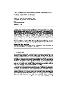
In order to compare the three approaches a simulation was created using NesC and TOSSIM 2.0, the most widely accepted sensor network simulator. The metric used was the total number of messages sent during equal periods of simulation. This was measured at various rates of application requests, sensor change, and application error percentages. Each simulation was run 20 times for 500 simulated seconds. The application requests were modeled by periodically choosing a mote and sensor and then requesting that value from the base station. Additionally, the performance at various levels of sensor error percentages were evaluated. Sensor values were created as a random walk with a parameterized change period. At each interval, the random walk will move up or down one unit, starting with a uniform distribution in the range of 150 to 250. A Normal distribution was used for the data model as a random walk distribution converges to a Normal distribution with mean of the initial value and variance of number of steps multiplied by the square of the step size. The mean was taken to be the current value and the number of steps was determined by the range allowed by the sensor error percentage. In practice, any data model can be used since our approach does not rely on a specific data model. Experimental Results: Figure 3 shows the behavior of the three methods when the rate of data change is varied. The simulations showed that HYBRID sends fewer messages than QDU-ONLY in cases of higher application request rates and better than SDU-ONLY for faster rates of data change. As is expected, QDU-ONLY does not change significantly with the rate of data change, and SDUONLY decreases dramatically as the rate of data change decreases. HYBRID is affected by this rate of change, but not to the extent that the SDU-ONLY is affected. As the frequency of change slows down, there is a point at which SDU-ONLY will send fewer messages than HYBRID. One reason for this is that when the sensor data change rate approaches the point that queries are never more efficient, both SDU-ONLY and HYBRID will send an update if the sensor value exceeds the error bounds, but HYBRID additionally sends an update if the validity expires. Figure 4 shows the behavior of the the three methods when the rate of application requests is varied. As expected, SDU-ONLY is not affected by the application request rate, and QDU-ONLY dramatically decreases messages sent as the frequency diminishes. HYBRID also decreases greatly as the frequency diminishes, however not at the same rate as QDU-ONLY. Shown in this figure is the point where QDU-ONLY will be more efficient, however the approaches remain competitive thereafter. Both HYBRID and QDU-ONLY decrease along an exponential curve as the application request period increases, however the QDU-ONLY is a steeper exponential curve. One reason for this is that the HYBRID approach uses the average number of queries in deciding whether to send an update or not, the more queries that are sent pushes the HYBRID approach back toward using sensor driven updates. Figure 5 shows the behavior of the three methods when

Figure 3: Impact of data change rate on the data collection overhead (query period = 1 s, application error percentage =3%) with 95% confidence interval.

Figure 4: Impact of application request frequency on the data collection overhead (sensor change period = .3 s, application error percentage = 3%) with 95% confidence interval.

the application error percentage is varied. As expected, QDU-ONLY is not affected by the change. Both SDUONLY and HYBRID are affected by the change in the error percentage, however similarly to the change in sensor period, the SDU-ONLY mode is affected more than the HYBRID method. In fact, the HYBRID method appears to level out as the sensor percentage grows large. This indicates that for larger error percentages SDU-ONLY will outperform HYBRID. However, for more stringent percentages, such as 3% or 5%, HYBRID will outperform or be competitive with SDU-ONLY. For percentages greater than this, it would be better to use an approach such as SDU-ONLY. The reason for this is similar to the reason a longer sensor change period benefits SDU-ONLY more

than HYBRID. Whether a larger error percentage or a longer average sensor change period, the length of time that the value will likely remain in range increases.

same observation. For instance, a potential fire breakout may be identified when 80% of nodes report their temperature readings over 100 degrees. Without loss of generality, an event is identified when a certain percentage (α%) of nodes report their readings over a threshold. Furthermore, in order to enable a prompt response to the event, these sensor reports must reach the base station within a reasonable timeframe (D time units). Thus, a WSN application requires α% of sensor reports within D time units for an event detection while minimizing energy consumption. Existing work mostly considers reliability, timeliness and energy consumption largely in isolation. Few attempts have been made to satisfy these requirements simultaneously. This simultaneous satisfaction imposes several challenges. First, reliability and timeliness are two competing goals. The requirement on reliability (i.e., the number of sensor reports) ensures that the base station can have enough information to make informed decisions on a detected event. The requirement on timeliness (i.e., deadline) aids timely decisions on a detected event. In order Figure 5: Impact of application error percentage on the data to ensure reliable data delivery, hop-by-hop recovery is ofcollection overhead (query period = 1 s, sensor data change ten applied; however, this may not meet a given timeliness requirement. Second, reliability and energy efficiency period = .1 s) with 95% confidence interval. conflict with each other. The more data the base station As stated previously, our approach also works for multi- receives, the more reliable decisions can be made based on hop networks. To keep it simple, our evaluation so far has the data; however, more energy is consumed for extra data only been conducted on a one-hop network, intending to retransmissions and recovery actions. Third, there exists merely validate our approach. In practice, many sensor a tradeoff between timeliness and energy efficiency. In ornetworks use clustering based or multi-hop based commu- der to detect an event sooner, more energy is drained from nication. To obtain results for non one-hop networks, a nodes because more data transmissions are required. We address the above challenge by designing WSN apfew key changes would need to be made. The relaying nodes could evaluate if adding their data to relayed pack- plications after biological systems. This design strategy is ets would be efficient. Furthermore, nodes that do not motivated by an observation that various biological syscommunicate directly with the base station would require tems have developed the mechanisms to meet conflicting either to develop a protocol or to have a MAC layer that requirements simultaneously. For example, a bee colony would provide an adequate estimate of energy used to send simultaneously maximizes the amount of collected nectar, a message to or receive a message from base station. Many maintains the temperature in a nest, and minimizes the strategies are available for such information, however, they number of dead drones [Seeley (2005)]. If bees focus only may require additional energy being spent due to increased on foraging, they fail to ventilate their nest and remove packet size or administration messages. A finished solution dead drones. Given this observation, this paper proposes to this problem is out of the scope of this paper, but we a biologically-inspired architecture for WSN applications would like to use the presented ideas to demonstrate that to adaptively balance the tradeoffs among conflicting reexploiting application’s error tolerance can help conserve quirements. The proposed architecture models each WSN application energy consumption and also validate applications’ data as a group of multiple mobile agents. This is analogous models. to a bee colony (application) consisting of bees (agents). Agents read/collect sensor data (as nectar) on individual 4 Case Study Two: Supporting Multiple Quality Needsnodes (modeled as flowers), and carry (or push) the data through multiple hops to the base station, which is modeled as a nest of bees. If they do not satisfy a desired In this section, we use composite need of reliability and level of reliability (i.e., the number of sensor data required timeliness as an example to demonstrate how multiple for an event detection), extra agents leave the base staquality constraints can be met while conserving energy tion (nest) to the network for collecting (or pulling) extra consumption. WSNs are often deployed to detect events sensor data from nodes. Agents perform these push/pull that are distributed spatially such as fire spreading and oil functionalities by invoking biologically-inspired behaviors spills. Due to the sheer number of sensor nodes and con- such as migration, swarm formation and replication. stant failures in the network, the detection of an event is ofIn order for agents to optimally perform their behavten determined when a certain number of nodes report the iors in terms of reliability, timeliness and energy efficiency,

agent behaviors are formulated into a well-known NP-hard problem, the Vehicle Routing Problem (VRP). Agents perform a decentralized and centralized VRP heuristics to push and pull sensor data, respectively. Simulation results show that the VRP-formulated migration behavior allows agents (i.e., WSN applications) to adaptively balance the tradeoffs among reliability, timeliness and energy efficiency and outperform an existing similar mechanism. 4.1

Problem Formulation

This paper assumes WSN applications, each of which requires the base station to collect at least NR sensor data within D time units. NR is referred as the desired reliability. Nrd (the actual reliability) denotes the actual number of data received by the deadline. In order to reliably detect an event, Nrd ≥ NR . In other words, each WSN applicard tion requires the normalized reliability N NR ≥ 1 while minimizing energy consumption. In order to formally state the problem at hand, we use the following notations to describe WSNs. A WSN is considered as a graph G(V, E). • V = {v0 , v1 , ..., vn } is a vertex set, where v0 is the base station. V ′ = V − {v0 } is a set of n sensor nodes. Each node periodically generates sensor data. • E = {(vi , vj )|vi , vj ∈ V ; i 6= j} is an edge set. An edge is established from the node vi to vj if vi can transmit a packet to vj . Due to the nature of asymmetric communication in WSNs, an edge is directed; (vi , vj ) ∈ E does not necessarily mean (vj , vi ) ∈ E. • cij is a non-negative weight associated with the edge (vi , vj ). It represents the cost for moving an agent between the nodes vi and vj . We will later describe the cost function to determine cij . • tij is the latency for an agent to move from the node vi to vj .

it. The goods are stored at a depot, where a fleet of vehicles is stationed. Vehicles have the identical maximum weight capacity and maximum route time (or distance) constraints. They must all start and finish their routes at the depot. It is assumed that Qi is less than the maximum weight capacity of each vehicle and Qi is delivered by a single vehicle. In VRP, both the required number of vehicles and their routes are unknown. The objective of VRP is to obtain a set of routes for vehicles to minimize their total route time. In fact, VRP is an m-TSP problem with two additional constraints: the maximum weight capacity and maximum route time for each vehicle. In our problem, there are n sensor nodes (demand points) in the network. Each node vi has a sensor data of size li bytes to be delivered to the base station (the depot) by an agent (an vehicle). The packet size limitation in WSNs is analogous to the vehicle weight capacity in VRP. The timeliness constraint in WSNs is mapped to the maximum vehicle route time in VRP. Cost Function: We next define the function to determine the link cost between the node vi and vj (cij ). We use packet loss rate to determine link cost. To avoid the asymmetric nature of communication links, the link cost cij is determined as fij × fji , where fij is the loss rate to transmit packets (agents) from the node vi to vj . Packet loss rate simultaneously impacts the reliability, timeliness and energy efficiency of sensor data transmission (agent transmission). Lower packet loss rate better meets all of the three requirements. Packet loss rate is measured when nodes are deployed. Currently, assuming that WSNs are semi-static [Woo et al. (2003); Meliou et al. (2006); Zhao and Govindan (2003), packet loss rate is measured at the beginning of a WSN operation. It can be periodically measured and updated; however, it is out of this paper’s scope. Each node transmits a set of packets to each neighboring node. Each packet contains its sequence number and the total number of transmitted packets. Upon receiving a set of packets, each neighboring node determines packet loss rate based on the number of received packets.

• m is the number of agents. Each agent can carry a limited size S of data due to the limitation of packet size. This is a constraint on how many nodes an agent can collect data from. 4.2 • Rk is a migration route for the agent k to follow. CRk is the cost P of moving the agent k along the route Rk . CRK = (h,h′ )∈Rk chh′ ; h′ is the next hop node of the node h in the route Rk .

Biologically-inspired Mobile Agents

In order to solve the problem at hand, this paper proposes to use biologically-inspired mobile agents in a push and pull hybrid manner. There are two types of agents: event agents and query agents. An event agent (EA) is deployed on each node. It carries (or pushes) a sensor data to the • TRk is the latencyPfor the agent k to move along the base station using multiple hops. On its way to the base route Rk . TRk = (h,h′ )∈Rk thh′ . station, each EA swarms with other EAs to aggregate as The problem at hand is to, given a set of n nodes, de- many sensor data as possible as long as it meets a given rd termine a set of m agents that can satisfy N 1 and deadline. Due to inherent failures in WSNs, EAs may not NR ≥P the migration route (Rk ) of each agent such that CRk be able to satisfy the desired reliability (the number of is minimized subject to max TRk ≤ D. sensor data required for an event detection). In this case, We can reduce this problem to Vehicle Routing Problem query agents (QAs) are created at the base station and dis(VRP). VRP can be described as follows. Let there be n patched to the network for collecting (or pulling) missing demand points in a given area, each demanding a quantity sensor data from nodes. Agents (EAs and QAs) implement of weight Qi (i = 1, 2, · · · , n) of goods to be delivered to the following behaviors.

• Replication: Agents (EAs and QAs) may make a copy of themselves. An EA replicates itself on a node when it detects an event of interest, which is applicationspecific and may simply be a sensor reading exceeding a threshold. A replicated EA contains collected sensor data can carries to the base station. A QA is replicated at the base station and dispatched to the network to collect sensor data from nodes. • Swarming: Agents (EAs and QAs) may swarm (or merge) with other agents on their way to the base station. EAs swarm with other EAs, and QAs swarm with other QAs. With this behavior, multiple agents become a single agent. The resulting (swarm) agent aggregates sensor data. This data aggregation saves power consumption of nodes because in-node data processing requires much less power consumption than data transmission does. • Migration: Agents may move from one node to another. Migration is used to deliver agents (sensor data) to the base station. There are two ways for agents to move. – Chemotaxis walk: The base station periodically propagates base station pheromones to individual nodes in the network. Their concentration decays on a hop-by-hop basis. (Each pheromone evaporates in a certain time period.) Agents (EAs and QAs) can locate the base station approximately, and move to the base station in the shortest paths by sensing pheromone’s concentration gradient. Base station pheromones are designed after the Nasonov gland pheromone, which guides bees to move toward their nest [Free and Williams (1972)]. – Sidestep walk: In addition to the chemotaxis walk, each EA may sidestep the shortest migration path and move to a neighboring node that has the equal or longer distance to the base station, as long as the EA meets a given deadline to reach the base station. This behavior encourages EAs to perform swarming-based data aggregation by increasing the number of nodes EAs visit. QAs are not allowed to perform this behavior. Agents perform their behaviors with VRP heuristics. We propose a decentralized VRP heuristics for EAs, and leverages an existing centralized VRP heuristics for QAs. Particularly, these VRP heuristics are used to answer the following questions. (1) Where and how should EAs replicate themselves? (2) How many agents (EAs and QAs) should be created? (3) How should each agent (EA and QA) move? A decentralized VRP heuristics for Event Agents: EAs implement a decentralized VRP heuristics to carry sensor data to the base station by a given deadline. To the best of our knowledge, there is no existing heuristics

to solve VRP in a decentralized way. We propose a decentralized greedy algorithm to govern the EA behaviors. The proposed algorithm uses a cluster-based approach to determine where and how EAs replicate themselves. Nodes are grouped to form clusters, and an EA replicates itself on each cluster head when it detects an event. Each cluster has one-hop topological radius, and all neighboring nodes of a cluster head become its cluster members. Cluster head election is designed to maximize the number of cluster members by choosing a sensor node who has many neighboring nodes. In this process, each node becomes idle first for Tidle time units. It calculates Tidle by randomly choosing a number between zero and Tmax /N . Tmax is a constant that specifies the bound of cluster head election period, and N is the number of neighboring nodes. After this idle period, each node becomes a cluster head and broadcasts an ADV (advertisement) message to its neighboring nodes. However, if a node receives an ADV message from any of its neighboring nodes during the idle period, it becomes a cluster member of the node who originates the ADV message. Each cluster member sends a JOIN message to its cluster head so that the cluster head know who are cluster members. Through this process, clusters are uniformly distributed and cover the entire network. Note that each node always belongs to a single cluster; if it receives multiple ADV messages during its idle period, it responds to the first ADV message and ignores subsequent ones. When an EA detects an event on a cluster head, the EA replicates itself one or more times. The replicated EAs visit cluster members to collect sensor data from them. This way, each EA aggregates sensor data and carries the aggregated data to the base station. The ideal number of replicated EAs per cluster is ⌈ ns ⌉, where n is the expected number of nodes in a cluster and s is the number of data that a single EA can carry. If an EA already contains s number of data and cannot contain any more, the EA is refereed as a fat EA. If an EA can still contain data, it is referred as a slim EA. Each fat EA moves toward the base station on a hop by hop basis by selecting the next hop node that minimizes the link cost (cij ). This allows fat EAs to increase the chances to reach the base station by a given deadline. By default, each slim EA also chooses the next hop node that minimizes link cost as well. However, when it finds a cluster on its way to the base station and has not visited the cluster’s head node, the EA sidesteps to the cluster head for swarming with other slim EAs as as far as it meets a timeliness constraint. If there is no slim EAs on the cluster head, the EA stays there for a period of time before moving to the base station again. This period increases the chances for a waiting EA to swarm with other slim EAs while allowing it to reach the base station within a given time constraint. The waiting period of each slim EA is calculated by each cluster head based on a given deadline and the latency from the cluster head to the base station. Let Td be the deadline, and ti,b be the latency from the cluster head i to the base

station, a slim EA at cluster head i can wait for Td − ti,b before it starts moving towards the base station. This waiting time allows slim EA to move to the base station within the deadline, as long as the deadline is greater than the longest traveling time. In addition, the waiting time allows slim EAs to increase the chance to combine with other slim EAs. For instance, we assume that on its way to the base station, a slim EA at cluster head i has to visit cluster head j which also has a slim EA. Let ti,b and tj,b be the latency from the cluster head i and j to the base station respectively. The traveling time from the cluster head i to j, ti,j , is then approximately ti,b − tj,b . The slim EA at cluster head i will wait until Td − ti,b , while slim EA at cluster head j will wait until Td − tj,b . When slim EA at cluster head i starts moving at Td − ti,b , it will reach cluster head j at time Td − ti,b + ti,j . This is the same as the time that slim EA in cluster head j is supposed to leave, which is Td − tj,b . So, the two EAs will combine and then leave cluster head j. This waiting and combination process is performed repeatedly along the way to the base station. In practice, the waiting time can be considered as an upper bound instead of a hard deadline. Therefore, an EA may leave a cluster head before the waiting time expires. A centralized VRP heuristics for Query Agents: QAs implement a centralized VRP heuristics to visit a certain number of nodes from the base station and collect extra sensor data on the nodes. To find an optimal number of QAs and also traveling path of each QA, Clarke-Wright Savings algorithm [Clarke and Wright (1964); Lenstra and Kan (1981)], a well known VRP solving algorithm, is used with some modifications. The Clarke-Wright Savings algorithm is an heuristic algorithm which uses constructive methods to gradually create a feasible solution with modest computing cost. Basically, the Clarke-Wright Savings algorithm starts by assigning one agent per vertex in the graph. The algorithm then tries to combine two routes so that an agent will serve two vertices. The algorithm calculates the “savings” of every pair of routes, where the savings is the reduced total link cost of an agent after a pair of route is combined. The pair of routes that have the highest saving will then be combined if no constraint, time or capacity, is violated. In this paper, Clarke-Wright Savings algorithm is extended to consider the time and space constraint. By looking into the data the base station has received from the EAs, the base station can determine to which cluster or area a QA should be dispatched initially. • An internal path, Rj , is created within each cluster, Xj which sensor readings are missing. Consider a set of node {v|v ∈ Xj }, Clarke-Wright Saving can be used by choosing a cluster head, i.e. swarm location, vˆj as a depot, then create a path to visit every v ∈ Xj − {ˆ vj }. The time, tj , to travel within the cluster is also assigned to the cluster.

• The cluster head, vˆi , is selected from the cluster Xj to represents the location of the cluster. • The shortest route Ri j between two nodes, vˆi and vˆj where i 6= j are calculated using Floyd-Warshall algorithm. The distance between nodes are measured by cost, cˆij of moving agent between two nodes, which is the function of packet loss rate. • A route R0j is created from base station to each node vˆj . • The saving of combining a pair of routes between the base station and two individual nodes(ˆ vj ; cluster representative) are computed. sij = cˆ0i + cˆ0j − cˆij

(2)

The saving must obey two constraints; first, the traveling time along the combining route must less than deadline, t0i + ti + tij + tj + tj0 < D and the number of node in the route R0ij , |Xi | + |Xj |, is less than space limit, S. • The saving is ordered from the largest to smallest into a saving list • Begin at the top of the saving list, a sub-tour is formed by merging the routes, R0i and R0j , that create the saving, sij ; – a new route, R0ij is constructed with traveling cost cˆ0ij and time t0ij . – the route R0i and R0j are removed. • The process is repeated from the first step until no more possible saving. Finally, a set of routes between cluster are constructed and an QA is assigned for each route. Also, the traveling route inside each cluster is given to a QA who is going to visit the cluster. Then, QAs are dispatched to collect data from each cluster by visiting the cluster head first.If QA can visit cluster head and the cluster head still have the sensor readings from each cluster members, QA can collect sensor readings from the cluster head and travel back to the base station immediately. However, if QA cannot visit the cluster head, e.g. cluster head is missing or running out of battery, QA then consult the traveling path inside the cluster which assigned by base station to visiting each cluster member to collect data and then travel back to base station. 4.3

Performance Evaluation

The proposed approach is implemented in NesC and evaluated using TOSSIM 1.0 [Levis (2003)]. A sensor network is simulated in an area of 200x200 square meters. In most of our experiments, the network consists of 150 sensor nodes modeled after MICAz mote with communication radius of about 30 meters, bandwidth of approximately 200kbps

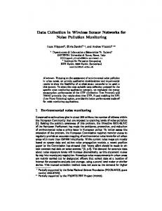
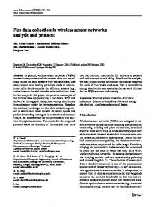
when the desired reliability is high (i.e. 1.0) proposed approach has lower energy consumption due to the data aggregation mechanism used in proposed approach. Figure 8 shows that the energy consumption of MMSPEED is constant regarding the desired reliability. Nevertheless, proposed approach can reduce the energy consumption when the desired reliability is low, i.e. by using only EAs.

Reliability by Deadline 1

Agentilla - 0.5 Agentilla - 1.0 Baseline - 0.5 Baseline-1.0 MMSPEED - 0.5 MMSPEED-1.0

Deadline(second)

0.95 0.9 0.85 0.8 0.75 0.7 0.65 60

70

80

90

100

Actual Reliability Figure 6: Impact of desired reliability on the actual reliability with varied deadline

Energy Consumption by Deadline 750 700

Deadline(second)

and 128kB of memory space [Crossbow Technology Inc. (2006)]. B-MAC is used as the MAC layer protocol by using CC2420 radio module in TinyOS. The sensor nodes are uniformly deployed in the area. To the best of our knowledge, only MMSPEED satisfies reliability and timeliness requirements simultaneously [Felemban et al. (2005)]. MMSPEED provides active ontime reachability of packets by using multiple speed levels and multi-path routing. It uses SPEED [He et al. (2003)] for the timeliness guarantee and adds probabilistic reliability guarantee based on probabilities of reliable delivery of packets at different links. MMSPEED provides the flexibility for applications to choose several different levels of reliability and timeliness. However, it does not consider minimizing the energy consumption in routing. Therefore, we implemented MMSPEED in TinyOS for comparison. In addition, we use TinyOS’s Drain Data Collection Protocol [Tolle and Culler (2005)] as a baseline. The application’s desired reliability is varied from 0.6 to 1.0 and desired freshness, which is a metric to measure timeliness, is varied from 60 and 100 seconds. Each sensor node reports sensing values one at a time and each agent can carry up to 10 readings. We evaluate the system performance to demonstrate how proposed approach achieves the desired reliability, freshness and the energy consumption involved. For Agentilla, the energy consumed during both the cluster formation stage and the data collection stage is included in the measurement. We have also studied how the network density, the packet size, i.e. the maximum number of sensor readings an agent can carry, and network fault severity affect the system performance. More results can be found in [Boonma et al. (2007)]. Figure 6 shows the actual reliability against the desired reliability when desired reliability is set to be 0.5 and 1.0. The results show that for proposed approach, a reliability of 0.74 can be achieved by purely using EAs. When the desired reliability is greater than 0.74 (i.e., 1.0), QAs are dispatched to collect additional data in order to archive higher reliability. However, due to the time constraint imposed by the application, the actual reliability can be less than the desired reliability. For example, when the freshness is very short (60 seconds in the figure), the highest achievable actual reliability is 0.81, which may be lower than the desired reliability. However, if the freshness is long enough, i.e. 90 - 100 seconds, the actual reliability can be equal or higher than the desired reliability. In contrast, Drain and MMSPEED can not improve the actual reliability beyond 0.73 and 0.85 respectively because both of them rely purely on push mechanism. Figure 7 shows the average energy consumption when the desired reliability is set to be 0.5 and 1.0. When the desired reliability is greater than 0.7, data collected by EAs can not satisfy the desired reliability, so the QAs are dispatched to gather additional data; hence, the increase in the total energy consumption. Compared with Drain and MMSPEED which consume similar amount of energy irrespective of any reliability requirement, our approach consume less energy when the desired reliability is low (i.e. 0.5). Moreover,

650 600

Agentilla - 0.5 Agentilla - 1.0 Baseline - 0.5 Baseline-1.0 MMSPEED - 0.5 MMSPEED-1.0

550 500 450 400 350 300 60

70

80

90

100

Average Energy Consumption (mJ) Figure 7: Impact of desired reliability on energy consumption with varied deadline

5

Suggestions for Future Research Directions

Existing work has largely been limited to studying the tradeoff between energy consumption and each individual quality need. The techniques developed differ in their assumptions about the observed phenomena, the network properties, and the stringency of application needs. Some

Average Energy Consumption (mJ)

Energy Consumption by Reliability 750 700 650 600 550 500 Agentilla - 0.5 Agentilla - 1.0 Baseline - 0.5 Baseline-1.0 MMSPEED - 0.5 MMSPEED-1.0

450 400 350 0.5

0.6

0.7

0.8

0.9

1

Reliability Figure 8: Impact of desired freshness on energy consumption with desired reliability

schemes are implemented at the data management layer, completely oblivious of underlying network routing or node duty cycling issues. Other schemes, in contrast, provide a universal routing protocol that does not take into account applications’ specific characteristics. We believe that all the non-functional needs (reliability, timeliness, and accuracy) are cross-cutting issues that are best addressed by cross-layer approaches. The dynamic and uncertain nature of sensor environments caused by varying network conditions, system loads and application traffic implies that data collection techniques must be adaptive and customizable to provide desired QoS and QoD. Collection of raw or derived data should take into account (a) the non-functional requirements of applications, (b) the underlying observed physical phenomena, whose properties may suggest a processing strategy, and (c) the characteristics and current state of the sensor network, e.g., its scale, degree of heterogeneity, processing/memory/energy capabilities of sensors. Considering the wide use of sensor data collection protocols as a building block for many sensor applications, the sensor network community needs to standardize a common methodology that evaluates these protocols. Despite a considerable number of proposed sensor data collection protocols in the literature, no comprehensive comparative analysis has been previously conducted. Those protocols are often designed with different assumptions and evaluated under different network and system conditions. The lack of a thorough and fair comparison among these protocols makes it very difficult for application developers to select an appropriate protocol for their applications. There is an urgent need to design a platform that allows both functional and non-functional (timeliness, accuracy, reliability) requirements of applications to be specified, simulates various network conditions and application workloads to be used for evaluation, and provides well-defined interfaces for easy plug-in of various schemes. This motivation is derived from the premise that choosing between compet-

ing execution strategies should be hidden from the user. Instead, user tasks will be submitted in a high-level language appropriate to the application domain. These will be mapped to appropriate data management primitives by the application software which will then be posed to the sensor database management system in a declarative (e.g., SQL-like) language. The language will specify not only what they need, but also in what manner they need the data. Subsequently, the application needs will then be evaluated by sensor data collection schemes. With the evaluation framework in place, we would be able to provide fair comparisons of existing sensor data collection protocols and thorough evaluation of any newly proposed techniques. The framework can also provide an end-to-end support of sensor data collection with varying QoS and QoD needs. A full-fledged framework can be built on initial work on data quality specification Bisdikian et al. (2009) and our previous work on Quality-aware Sensing Architecture (QUASAR) Lazaridis et al. (2004).

ACKNOWLEDGMENT

We would like to thank Iosif Lazaridis, Sharad Mehrotra, and Nalini Venkatasubramanian for early discussions on related topics that have inspired the work presented here. This work is supported in part by NSF CSR grant CNS-0720875.

REFERENCES

Bisdikian, C., Kaplan, L. M., Srivastava, M. B., Thornley, D. J., Verma, D., and Young, R. I. (2009). Building principles for a quality of information specification for sensor information. In Proceedings of the 12th International Conference on Information Fusion. Boonma, P., Han, Q., and Suzuki, J. (2007). Leveraging biologically-inspired mobile agents supporting composite needs of reliability and timeliness in sensor applications. In Proceedings of IEEE International Conference on Frontiers in the Convergence of Bioscience and Information Technologies (FBIT), pages 851–860. Chakravarthy, S., Krishnaprasad, V., Anwar, E., and Kim, S. (1994). Composite events for active databases: Semantics, contexts and detection. In Proceedings of the International Conference on Very Large Data Bases (VLDB). Clarke, G. and Wright, J. W. (1964). Scheduling of vehicles from a central depot to a number of delivery points. INFORMS Operations Research, 12(4):568–581. Crossbow Technology Inc. (2006). Micaz datasheet. Deligiannakis, A., Kotidis, Y., and Roussopoulos, N. (2004). Hierarchical in-network data aggregation with quality guarantees.

Demers, A., Gehrke, J., Rajaraman, R., Trigoni, N., and Lenstra, J. K. and Kan, A. R. (1981). Complexity of veYao, Y. (2003). The cougar project: A work-in-progress hicle routing and scheduling problems. Wiley Networks, report. ACM SIGMOD Record, 32(4). 11(2). Deshpande, A., Guestrin, C., Madden, S., Hellerstein, J., Levis, P. (2003). Tossim: Accurate and scalable simulation of entire tinyos applications. In Proc. of the 1st ACM and Hong, W. (2005). Model-based approximate queryConf. on Embedded Networked Sensor Systems. ing in sensor networks. The VLDB Journal, 14(4):417– 443. Lu, C., Xing, G., Chipara, O., Fok, C. L., and Bhattacharya, S. (2005). A spatiotemporal query service for Felemban, E., Lee, C., Ekici, E., Boder, R., and Vural, mobile users in sensor networks. In Proceedings of InterS. (2005). Probabilistic qos guarantee in reliability and national Conference on Distributed Computing Systems timeliness domains in wireless sensor networks. In Proc. (ICDCS). of the 24th Annual IEEE Conf. on Computer Communications.

Madden, S. R., Franklin, M. J., Hellerstein, J. M., and Hong, W. (2003). The design of an acquisitional query Free, J. B. and Williams, I. H. (1972). The role of the naprocessor for sensor networks. In Proceedings of ACM sonov gland pheromone in crop communication by honey International Conference on Management of Data (SIGbees. Int’l J. of Behavioural Biology, 41:314–318. MOD). Hakkarinen, D. and Han, Q. (2008). Data quality driven Meliou, A., Chu, D., Guestrina, C., Hellerstein, J., and sensor reporting. In Proceedings of the IEEE InternaHong, W. (2006). Data gathering tours in sensor nettional Conference on Mobile Ad Hoc and Sensor Systems works. In Proc. of Int’l Conf. on Info Processing in Sen(MASS), pages 772–777. sor Nets. Han, Q., Lazaridis, I., Mehrotra, S., and Venkatasubrama- Ozsoyoglu, G. and Snodgrass, R. T. (1995). Temponian, N. (2005). Sensor data collection with expected ral and real-time databases: A survey. Proceeding of reliability guarantees. In Proc. of the 1st IEEE Int’l IEEE Transactions on Knowledge and Data EngineerWorkshop on Sensor Networks and Systems for Pervaing (TKDE), 7(4). sive Computing. Park, S. J., Vedantham, R., Sivakumar, R., and Akyildiz, Han, Q., Mehrotra, S., and Venkatasubramanian, N. I. F. (2004). A scalable approach for reliable downstream (2004). Energy efficient data collection in distributed data delivery in wireless sensor networks. In Proceedsensor environments. In Proceedings of IEEE Interings of ACM International Symposium on Mobile Ad national Conference on Distributed Computing Systems Hoc Networking and Computing (MobiHoc). (ICDCS), pages 590–597. Porta, L., Illangasekare, T. H., Loden, P., Han, Q., and Jayasumana, A. P. (2009). Continuous plume monitorHan, Q., Mehrotra, S., and Venkatasubramanian, N. ing using wireless sensors: Proof of concept in inter(2007). Application-aware integration of data collection mediate scale tank. ASCE’s Journal of Environmental and power management in wireless sensor networks. J. Engineering. Parallel Distrib. Comput., 67(9):992–1006. He, T., Stankovic, J. A., Lu, C., and Abdelzaher, T. F. (2003). Speed: A stateless protocol for real-time communication in sensor networks. In Proc. of the 23rd IEEE Int’l Conf. on Distributed Computing Systems.

R. Cristescu and M. Vetterli (2005). On the optimal density for real-time data gathering of spatio-temporal processes in sensor networks. In International Symposium on Information Processing in Sensor Networks.

Hwang, I., Han, Q., and Misra, A. (2005). MASTAQ: A middleware architecture for sensor applications with statistical quality constraints. In Proceedings of IEEE International Workshop on Sensor Networks and Systems for Pervasive Computing (PerSeNS), pages 390–395.

Ramamritham, K. (1996). Real-time databases. International Journal of Distributed and Parallel Databases, 1(2).

Sankarasubramaniam, Y., Akan, O. B., and Akyildiz, I. F. (2003). Esrt: Event-to-sink reliable transport in wireless sensor networks. In Proc. of the 4th ACM Int’l SympoLazaridis, I., Han, Q., Mehrotra, S., and Venkatasubramasium on Mobile Ad Hoc Networking and Computing. nian, N. (2006). Fault-tolerant queries over sensor data. In Proceedings of International Conference on Manage- Seeley, T. (2005). The Wisdom of the Hive. Harvard Uni. ment of Data (COMAD). Press. Lazaridis, I., Han, Q., Yu, X., Mehrotra, S., Venkatasub- Sharaf, M., Beaver, J., Labrinidis, A., and Chrysanthis, ramanian, N., Kalashnikov, D., and Yang, W. (2004). P. (2004). Balancing energy efficiency and quality of Quasar: Quality aware sensing architecture. ACM SIGaggregate data in sensor networks. The VLDB Journal, MOD Record, 33(1):26–31. 13(4):384–403.

Sistla, A. and Wolfson, O. (1995). Temporal conditions and integrity constraints in active database systems. In Proceedings of ACM International Conference on Management of Data (SIGMOD). Tansel, A., Clifford, J., Gadia, S., Jajodia, S., Segev, A., and Snodgrass, R. (1994). Temporal Databases: Theory, Design and Implementation. Benjamin/Cummings. Tolle, G. and Culler, D. (2005). Design of an applicationcooperative management system for wireless sensor networks. In Proc. of European Workshop on Wireless Sensor Work. Woo, A., Tong, T., and Culler, D. (2003). Taming the underlying challenges of reliable multihop routing in sensor networks. In Proc. Int’l Conf. on Embedded Networked Sensor Sys. Zhao, J. and Govindan, R. (2003). Understanding packet delivery performance in dense wireless sensor networks. In Proc. of Int’l Conf. on Embedded Networked Sensor Sys.