by Deborah L. Kane, German A. Prieto, Frank L. Vernon, and Peter M. ...... Roy. Soc. Lond. Math. Phys. Sci. 241, 376â396. Frankel, A., and H. Kanamori (1983).
Bulletin of the Seismological Society of America, Vol. 101, No. 2, pp. 535–543, April 2011, doi: 10.1785/0120100166
Quantifying Seismic Source Parameter Uncertainties by Deborah L. Kane, German A. Prieto, Frank L. Vernon, and Peter M. Shearer
Abstract
We use data from a small aperture array in southern California to quantify variations in source parameter estimates at closely spaced stations (distances ranging from ∼7 to 350 m) to provide constraints on parameter uncertainties. Many studies do not consider uncertainties in these estimates even though they can be significant and have important implications for studies of earthquake source physics. Here, we estimate seismic source parameters in the frequency domain using empirical Green’s function (EGF) methods to remove effects of the travel paths between earthquakes and their recording stations. We examine uncertainties in our estimates by quantifying the resulting distributions over all stations in the array. For coseismic stress drop estimates, we find that minimum uncertainties of ∼30% of the estimate can be expected. To test the robustness of our results, we explore variations of the dataset using different groupings of stations, different source regions, and different EGF earthquakes. Although these differences affect our absolute estimates of stress drop, they do not greatly influence the spread in our resulting estimates. These sensitivity tests show that station selection is not the primary contribution to the uncertainties in our parameter estimates for single stations. We conclude that establishing reliable methods of estimating uncertainties in source parameter estimates (including corner frequencies, source durations, and coseismic static stress drops) is essential, particularly when the results are used in the comparisons among different studies over a range of earthquake magnitudes and locations.
Introduction The scaling of earthquake source parameters with magnitude has been a point of debate in recent years. This debate is motivated by the implications for understanding earthquake source physics. The issue is whether large earthquakes can be adequately approximated by linearly scaling the attributes of smaller earthquakes or whether something fundamentally differs in the rupture physics of different size earthquakes. Many studies have looked for evidence (or lack thereof) of self-similar source scaling (e.g., Abercrombie, 1995; Mayeda and Walter, 1996; Ide and Beroza, 2001; Ide et al., 2003; Mori et al., 2003; Prieto et al., 2004; Abercrombie and Rice, 2005; Imanishi and Ellsworth, 2006) by using a range of datasets and techniques, but many of these studies lack quantitative estimates of parameter uncertainties. Understanding the similarities and differences of earthquakes over a range of magnitudes is critical for earthquake source physics. Smaller earthquakes occur much more frequently than larger earthquakes, make up a much greater portion of the data collected, and allow a statistical consideration of source properties not achievable with individual large earthquakes. If there is something fundamentally different in the rupture physics of different size events, then our understanding of the hazard presented by large earthquakes will be inadequate. Accurately quantifying differences in earthquake source parameters should include consideration of the uncer-
tainties in each measurement (Abercrombie and Rice, 2005; Prieto et al., 2006). The heart of the source scaling question currently lies in how researchers estimate seismic source parameters, how these estimates are subsequently combined over varied datasets, and how magnitude scaling is evaluated (Abercrombie and Rice, 2005). Here we focus on the issue of possible magnitude scaling by considering the often overlooked uncertainties in the source parameter estimates. We approximate the uncertainties by studying the distribution of estimates over an array of closely spaced stations (distances ranging from ∼7 to 350 m). Differences in the propagation paths between a given source and all stations are very small because the spacing between the stations is small relative to the distance between the earthquake locations and the array (smallest source-station separation is 6.4 km). Azimuthal variations due to rupture directivity effects can likewise be ignored. The ground motions associated with an earthquake should be similar at each station because of this geometry, but local heterogeneities in near-surface structure could produce somewhat different waveforms across the array. This unique dataset allows us to constrain the uncertainties of our parameters at each station individually and gain some insight into the predicted variability for other data by analyzing the resulting estimates and their distribution. 535
536
D. L. Kane, G. A. Prieto, F. L. Vernon, and P. M. Shearer Small Aperture Array at PFO
The San Jacinto Fault Zone and the Small Aperture Array (SAA) Experiment 0
34.5
-50
34
-100
latitude
Distance (m)
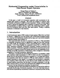
We use data from a high frequency array experiment installed in 1990 at Pinyon Flat Observatory (PFO) near the San Jacinto fault zone (SJFZ) in southern California (Vernon et al., 1991; Al-Shukri et al., 1995; Vernon et al., 1998, Wagner, 1998). Pinyon Flat is located on a pluton at the northern end of the Peninsular Ranges batholith in an area of nearly flat topography. Instruments were installed at the base of the uppermost weathered granodiorite layer, on top of the slightly more solid bedrock (Vernon et al., 1998, and references therein). This site was chosen as a location to test coherence of seismic waves over an array. The benefits of the site include easy accessibility, a hard rock region with relatively uniform geology, and minimal local topographic variation. Previous studies suggest that the weathered surface layer is heterogeneous with variable depth, and this layer acts as a waveguide for incident P waves (Al-Shukri et al., 1995; Vernon et al., 1998; Wagner, 1998). Wilson and Pavlis (2000) additionally showed that the variation in site responses across the array occurs on small distance scales of approximately the size expected for weathered granitic rocks. With the aim of studying coherence on a scale not previously attempted, the small aperture array (SAA) experiment (Owens et al., 1991) was installed for one month. The array consisted of 58 surface stations and 2 borehole stations. Thirty-six of the surface stations were placed in a square grid with ∼7 m spacing between adjacent stations. The remaining 22 surface stations extended in arms away from the square grid to the south and east using ∼21 m spacing between stations. The two borehole stations were placed near the center of the square grid at 150 m and 275 m depths in separate boreholes (Fig. 1). Three-component L22-D geophones (2-Hz response) and six-channel PASSCAL REFTEK RT72A-02 dataloggers were used at each of the SAA stations. The network was event-triggered at the deepest borehole station, and each station recorded ground velocity at 250 samples per second. These closely located stations recorded ground motion with visually similar waveforms across the array (Fig. 2). Using the array data in conjunction with data from the local ANZA network, 156 local earthquakes (M 0.8 to M 4.0) were initially identified and located. Many of these earthquakes occurred in clusters to the south and west of the array along the trace of the SJFZ. We estimate location uncertainties to be at least 1 km. Additional earthquakes were recorded but not initially located or assigned magnitudes. We estimate locations for these events using arrival lag times determined by waveform cross-correlation of the orthogonal arm stations in conjunction with S- and P-wave arrival-time differences. To assign magnitudes to these additional events, we determine a local scaling of magnitude as a function of source-station distance and peak amplitude. This process nets 55 additional earthquakes, bringing our catalog to a total of 211 local events (M 0.7 to M 4.0).
SAA
-150
33.5
-200 -118
-117.5
-117
-116.5
33 -116
longitude 0
50
100
150
200
250
Distance (m)
Figure 1. Map showing the small aperture array (SAA) station distribution (triangles), study area, and relocated seismicity (black circles). The SAA was installed along the SJFZ; mapped fault traces are shown as gray lines. Several small clusters of earthquakes are apparent in the map. Previous analysis of data recorded by SAA shows that coherence among stations rapidly decreases above 15 Hz at almost all length scales (Vernon et al., 1998). P- and S-wave coda analysis suggests the presence of localized heterogeneities in the near-surface structure (Wagner, 1998). Al-Shukri et al. (1995) reports evidence of significant frequency-dependent variations in the temporal and spectral domains and suggests that the differences can be explained by variations in the near-surface conditions.
Estimating Source Parameters We use frequency domain methods with empirical Green’s function (EGF) techniques to estimate corner frequencies and coseismic static stress drops from P-wave data. Methodology Seismic source parameters are routinely estimated in the frequency domain. We fit a Brune (1970) source spectrum model to relative source spectra Ω0 : (1) u�f� � 1 � �f=fc �2 In some studies, the value of the exponent in the denominator is allowed to vary between 1 and 3 to control how quickly the signal decays above the corner frequency, fc . Here the value of the exponent is set, and fc and the long-period amplitude, Ω0 , are fit to the data. Estimates of these spectral parameters can subsequently be used to estimate parameters not directly measurable in the data.
Quantifying Seismic Source Parameter Uncertainties
537
M 2.2 earthquake, 12.3 km from array
east arm
X6Y3 X7Y3 X8Y3 X10Y3 X11Y3 X12Y3 X13Y3 X15Y3 X16Y3
south arm
central square grid
X0Y0 X0Y1 X0Y2 X0Y3 X0Y4 X0Y5 X1Y0 X1Y1 X1Y2 X1Y3 X1Y4 X1Y5 X2Y0 X2Y1 X2Y2 X2Y3 X2Y4 X2Y5 X3Y0 X3Y1 X3Y2 X3Y3 X3Y4 X3Y5 X4Y0 X4Y1 X4Y2 X4Y3 X4Y4 X5Y0 X5Y1 X5Y2 X5Y3 X5Y4
X3Y6 X3Y7 X3Y8 X3Y9 X3Y10 X3Y11 X3Y12 X3Y13 0.1 s
Figure 2. Waveforms from an M 2.2 earthquake recorded by the SAA at an epicentral distance of 12.3 km. The closely spaced stations within the central square grid record very similar waveforms while the stations in the linear arms record somewhat less similar waveforms. Focal sphere effects can be neglected because the stations are very close to each other. One of the common parameters considered in the source scaling controversy is the coseismic stress drop, first formulated by Eshelby (1957), Δσ �
7 M0 : 16 r3
(2)
Here r is the radius of the earthquake’s assumed circular rupture patch. We can combine equation (2) with the predicted relationship between source radius and P-wave corner frequency given by Madariaga (1976), β fc � 0:32 ; r
(3)
where β is the S-wave velocity (the rupture velocity is assumed to be 0:9β). Doing so allows us to derive a relationship between stress drop and P-wave corner frequency, � � fc 3 : (4) Δσ � M0 0:42β Of special note in this formula is the cubic relationship of corner frequency with stress drop. We cannot measure stress drop for small earthquakes directly; instead, we must estimate it from other source parameters. Significant uncer-
tainties in the corner frequency estimates will result in subsequent large uncertainties in estimates of stress drop. Empirical Green’s Function Methods The ground motion, m, recorded at each station can be represented by a convolution of signals from the seismic source, s0 , from the effects of the travel path between the source and the recording station, p, and from the site and instrumentation effects at the station, i. This can be represented by m�t� � s0 �t� � p�t� � i�t�:
(5)
where � indicates convolution and each signal is a function of time. We use a small earthquake as an EGF to isolate the source term from the signal recorded for a larger, nearby earthquake (Hartzell, 1978). In doing so, we assume that: (1) the two earthquakes have the same radiation patterns, (2) the path and site effects are identical for both earthquakes because the earthquakes are approximately collocated, and (3) the EGF earthquake source can be treated as a point source because it is both smaller in size and shorter in rupture duration than the larger magnitude mainshock earthquake. Under these assumptions, we can rewrite equation (5) as m�t� � g�t� � s�t�:
(6)
Here g is the ground motion recorded for the EGF earthquake, and s is the relative source contribution of the two earthquakes. Pairs of closely located earthquakes are required for the EGF method to be successful, but not all of the earthquakes in our data catalog have an appropriate EGF earthquake. We restrict our mainshocks to earthquakes M ≥ 2 and pair these with EGF earthquakes that are at least one unit of magnitude smaller and within a hypocentral distance of 3 km of the mainshock event. These limits were chosen to accommodate as many mainshock–EGF pairs as possible given the geometry of the clustered events in our dataset and the event location uncertainties. We additionally constrain our data by only using mainshock and EGF earthquake pairs with similar S-to-P maximum amplitude ratios (mean value over the array must be within a factor of 2). This functions as a simple test of source mechanism similarity because significant differences in nodal plane orientation will produce large differences in these ratios. We require all seismograms used in our analysis to satisfy a minimum mean signal-to-noise ratio (SNR) of 3 for frequencies between 4 and 45 Hz. These requirements limit our usable data to a total of 7 mainshocks with 23 possible mainshock–EGF pairs. Frequency Domain We compute velocity spectra for 1-s windows by using multitaper spectrum estimation with six tapers (Park et al., 1987; Prieto et al., 2009). The frequency domain
538
D. L. Kane, G. A. Prieto, F. L. Vernon, and P. M. Shearer
representation allows us to write equation (6) as the multiplication of two spectra rather than the convolution of two time series: M�f� � G�f�S�f�:
(7)
We subsequently compute the spectral ratio of the mainshock to the EGF records at each station in order to remove the path and site effects and isolate the source spectrum, S�f�, of the larger earthquake. We do not filter the waveforms or smooth the spectra prior to computing the spectral ratio and fitting the model parameters. For each spectral ratio, we use unweighted least-squares estimation to fit a source model (equation 1) to the logarithm and determine the relative scalar seismic moment and corner frequency of the mainshock spectrum (Fig. 3). These fits are performed over the same frequency points at each station with the frequencies used in the inversion determined by signal-to-noise ratio tests. We require a minimum mean SNR of 3 as measured over 15 Hz bandwidths below 45 Hz. Estimates above 45 Hz are included when the SNR requirement is met over 5 Hz bandwidths at all stations satisfying the original 45 Hz criterion. Events with fewer than five stations meeting SNR requirements are excluded. The
spectral fits to the source models are relatively good for the individual spectral ratio measurements, and we find that the n � 2 model is adequate (Fig. 3). We do not fit the higher corner frequency of the EGF event because we expect these frequencies to be near or above the limitations imposed by SNR constraints, and we assume that deviations from a flat EGF source spectrum will be small in this frequency range. The mainshock corner frequencies estimated at each individual station exhibit variations across the array, although the spectral fits visually appear similar in log-space. While it is often a good practice to apply an inverse weighting with frequency to this inversion (e.g., Prejean and Ellsworth, 2001; Ide et al., 2003) to account for the large number of samples at high frequencies, this method does not produce reliable spectral fits for this dataset. The spectral ratios tend to exhibit a characteristic dip between 10 and 20 Hz for most event pairs, and the inverse frequency weighting prioritizes this dip over the roll-off at higher frequencies. This spectral feature is consistent across the dataset and appears larger in some cases than in others. To test the robustness of individual corner frequency fits, we measure the spectral misfit while varying the corner
M 2.2 paired with M 0.9 EGF event
(a)
X0Y2 spectral ratio
10
(b)
X7Y3
4
102
100
source spectrum station fit, fc = 30.8 Hz array fit, fc = 32.6 Hz
source spectrum station fit, fc = 35.1 array fit, fc = 32.6 Hz
(c)
X3Y11
(d)
spectral ratio
104
102 array fit, fc = 32.6 Hz weighted fit, fc = 24.8 Hz all stations, fc = 31.0 ± 4.2 Hz
source spectrum station fit, fc = 21.5 Hz array fit, fc = 32.6 Hz
100 0 10
101 frequency (Hz)
102
100
101 frequency (Hz)
102
Figure 3. Example source spectrum fitting for one earthquake pair. Spectra plotted in the lightest shade show the mainshock/EGF spectral ratio at a single station in (a) the central square grid, (b) the east arm, and (c) the south arm. The thin gray curve shows the spectral fit for that single station with corner frequencies given in the legends. These fits are performed over the same band at each station with the maximum frequency determined by SNR limits. The spectral fit obtained using all stations simultaneously without weighting is plotted as the thick black line in each subplot. In (d), the spectral ratios used in the estimates (circles) and individual fits at all stations (thin gray lines) are shown. The dashed line in (d) shows the simultaneous spectral fit obtained when using weighted least-squares, with the weighting given by the variance of the amplitudes at each frequency. The spectral ratio shown in gray is from the deeper borehole sensor; the shape is comparable to those of the surface stations but the borehole sensor records are excluded from the inversion.
Quantifying Seismic Source Parameter Uncertainties frequency and relative seismic moment around each original estimate. Viegas et al. (2010) used a similar grid search technique to constrain source parameter estimates within a 5% increase in fit variance. We apply a comparable limit by measuring corner frequencies at a spectral misfit increase of 5% from the original fit to obtain confidence intervals for each estimate. We obtain a more stable estimate of these source parameters by also fitting for relative moment and corner frequency simultaneously over all stations in the array using an unweighted least-squares inversion. This method produces array fits very similar to the individual station fits. Performing the array inversion using weighted least-squares, with weighting given by the variance of the amplitudes at each frequency point, results in consistently higher relative moment estimates and lower corner frequency estimates (Fig. 3). This is due to the smaller variation of amplitudes exhibited at lower frequencies as compared with the noisier high frequency amplitudes. The stations are very close together relative to the distance between the earthquakes and the array, allowing us to ignore any potential complications of azimuthal variations in the source when considering all stations in the array simultaneously. Thus, we focus on the differences in the results obtained for the different stations while recognizing that the single takeoff angle sampled is an incomplete representation of the source. With an azimuthally distributed array, such simultaneous spectral fitting should average any variations due to rupture directivity and differences in mainshock and EGF radiation patterns. The change to the overall spectral fit and subsequent change in stress drop estimates due to using weighted least-squares demonstrates that differences in fitting methods may introduce strong biases in the results. Our corner frequency estimates are consistent with those from previous studies for earthquakes in this magnitude range and region (Prieto et al., 2004). The distribution of individual station estimates has a consistent spread over the range of magnitudes considered after normalizing by the mean corner frequency estimate for each event. The variations in these estimates are not due to the contribution of a single event alone. We do not draw conclusions on the presence or lack of earthquake self-similarity due to the limited range of magnitudes in our selection of mainshock earthquakes (2:0 < M < 3:4) and narrow azimuthal coverage. These frequency domain methods are commonly used to estimate earthquake source parameters, but they suffer from several limitations and require assumptions that are not always testable. The spectral model assumes a circular, shear rupture at the source. The EGF technique assumes that mainshock and EGF earthquakes are collocated (rarely the case in most datasets) and that the event pairs chosen have identical source radiation patterns. Finally, these methods require the difference in corner frequencies between the mainshock and EGF earthquakes to be large enough to resolve. If the corner frequencies are too close to each other, then the mainshock corner frequency estimates will be biased.
539 Stress Drop We treat the cataloged local magnitudes as moment magnitudes to determine seismic moments for computing stress drops (equation 4). While these magnitude scales are likely not equivalent in this magnitude range (e.g., Shearer et al., 2006), we assume that the appropriate scaling is the same for all events. As our primary focus is on examining the distribution of estimates over the array for each mainshock earthquake, any differences from the absolute moments will not affect our results. Indeed, we find that the stress drops determined from these assumptions are higher than might be expected from other studies with a median value of 115 MPa. These differences could be attributed to our treatment of local magnitudes as moment magnitudes, truly higher stress drops in the region (Frankel and Kanamori, 1983; Prieto et al., 2004), or source effects (e.g., rupture directivity) that affect the corner frequency results due to the narrow source-array azimuth we are considering. Stress drops computed from the array spectral fits are somewhat lower than those resulting from the individual station estimates. The small range of earthquake magnitudes in our dataset limits our abilities to determine if stress drop scaling is constant or varying with earthquake magnitude.
Uncertainties in Source Parameter Estimates Our primary goal in this study is to measure station-tostation variations in source parameter estimates in the small aperture array and assign an appropriate estimate of uncertainty for source parameter estimates at a single station. We limit our analysis to the surface stations and quantify variability in estimates of corner frequency by considering the percent deviation from the mean estimate over all stations for each pair of events. This normalization is necessary to reasonably compare variations in parameters estimated over a range of earthquake magnitudes. The distribution of percent deviation from the mean for corner frequency exhibits somewhat long tails (Fig. 4). We measure the width of this distribution with the interquartile range (IQR), which gives the difference between the third and first quartile. The IQR estimate is 23% for the corner frequency distribution. This means that if our distribution is exactly symmetric, then half of our data fall within the �11:5% of the mean corner frequency estimate for each pair. Looking in further detail at each of the individual 23 pairs of events shows that some pairs exhibit a much wider distribution of corner frequency estimates than others. These pairs are not limited to any particular mainshock or EGF earthquake and are likely due to matching mainshock earthquakes with EGF earthquakes that do not meet all of our EGF technique assumptions. Pairs have been excluded from our dataset based on the separation distance between the mainshock and EGF earthquake, signal-to-noise ratio limitations, and source similarity requirements; these remaining pairs successfully passed each of these tests. Examination of the spectra for the most
540
D. L. Kane, G. A. Prieto, F. L. Vernon, and P. M. Shearer Percent deviations from mean corner frequency estimates
Deviations from mean stress drop estimates 80
60
iqr = 0.31
iqr = 23.4% 70
50
60 40
count
count
50 30
40 30
20
20 10
10 0 −100 −80
−60
−40
−20
0
20
40
60
80
100
percent deviations
0 −1 −0.8
−0.6
−0.4
− 0.2
0
0.2
0.4
0.6
0.8
1
log stress drop deviations (MPa)
Figure 4. Distributions of percent deviations from the mean for corner frequency estimates.
Figure 5.
anomalous pairs of events shows that the spectra are not consistently fit over all stations due to complexity in the spectral shape, and the corner frequency is fit at different values depending on the station considered. To examine the degree to which including such pairs affects our results, we remove pairs of events that have IQR values greater than twice the mean IQR of the entire dataset. This process limits the dataset further to 21 pairs out of the total 23 considered previously. After removing these pairs from our dataset, the resulting distribution of corner frequency deviations for all remaining pairs decreases in width slightly from 23% to 22.5%. All following estimates include the outliers unless otherwise specified. Our corner frequency distributions generally fit a lognormal distribution regardless of inclusion or exclusion of the outlier pairs; the apparent skewness in the distribution is due to plotting the percent deviation. We do not observe any systematic dependence of distribution width on either mainshock magnitude or mainshock– EGF magnitude differential; this suggests that the variability we are measuring is due to variations at the stations rather than the sources. The sizes of the confidence intervals also show no strong dependence on event magnitude after normalizing by the corner frequency estimates. We find that the confidence intervals for each individual corner frequency estimate are generally larger than the width of the distribution describing the variation in estimates across the array. This suggests that estimating confidence intervals using the grid search method may provide a reasonable means of approximating the source parameter uncertainties in some cases. We consider stress drop deviations from the mean in the log-domain rather than by percent. For stress drop estimates determined from the frequency domain results, the logdomain IQR is 0.31 (Fig. 5). If we assume a symmetric distribution, then this corresponds to an uncertainty range of �0:15 on each log stress drop estimate to contain the middle
half of the data (e.g., an estimate of 1 MPa stress drop would be equivalent to 0 � 0:15 in the log-domain or error bars from 0.7 to 1.4 MPa in the linear domain). This value scales logarithmically when applied to absolute estimates and corresponds to an uncertainty range of 0.07 to 0.14 MPa for a mean stress drop estimate of 0.1 MPa and 7 to 14 MPa for a mean estimate of 10 MPa. Excluding the outlier pairs decreases the IQR by less than 0.01, demonstrating that our results are robust. These values suggest we should consider minimum uncertainties of � ∼ 30% for individual station estimates of stress drop, particularly because these uncertainty estimates are based on IQR estimates that are more conservative than one standard deviation.
Distributions of deviations from the mean stress drop estimates (in log-space) using frequency domain methods.
Variations due to Data Choice The variations we observe in source parameter estimates could have several origins. We verify that the variations seen in the source parameter estimates are not dominated by unusual source locations, large local site effect variations at a subset of the stations in the array, or choices of mainshock and EGF earthquake pairs. We review the variations of estimates in each of these populations to confirm that our results are not biased by a subset of our data. We do not observe a correlation between mainshock magnitudes and the subsequent distribution widths of the estimates. Station Location The location of individual stations in the array could contribute to the variations we see in the source parameter estimates if there are consistent variations in the very localized rock structure near a specific station. Previous work with this dataset has demonstrated a loss in coherence across the array above 15 Hz and suggested that small-scale variations in local structure affect the propagation of ground
Quantifying Seismic Source Parameter Uncertainties
541
motion significantly on the scale of station spacing in this array (Vernon et al., 1998). We compare the distribution of source parameter estimates from three different station groupings: (1) the central square grid, (2) the south arm, and (3) the east arm (Fig. 6). All three sets display relatively symmetric distributions of estimates, confirming that the distribution of results from the full array is not significantly affected by one of these groupings. The central square grid contains the highest number of stations and results in a much smoother distribution of estimates. We consider variations from the mean estimate for each mainshock–EGF earthquake pair on a station-by-station basis to look for site effects on a smaller scale than the footprint of the central grid and of the two arms (Fig. 6). Groupings of positively and negatively biased stations are apparent for each pair of events, but this pattern is not consistent when Deviations of corner frequency estimates
(a) 0.3
distribution
center grid 0.2
south arm east arm
0.1
0 −80
−40
−20
0
20
40
60
80
Average deviation from mean corner frequency estimate by station 100
North (meters)
Earthquake Pair Location We next check to see if variations in the distribution of source parameter estimates are related to a particular set of earthquake sources. We first look at the distribution of estimates from nearby earthquakes (within 30 km of the array) and compare these estimates with those from more distant earthquakes. We do not find a consistent difference between the distributions of these two populations. Additionally, the closest and farthest events from the array do not appear to give substantially different results, confirming that we are not merely measuring uncertainties due to signal quality. We also look at the distribution of estimates based on source-station azimuth to check if earthquakes from one source location produce results differing considerably from those in a different source region, which would skew our resulting distribution. Again, we do not find consistent variations in the distribution of estimates from these groups. The location of the earthquake pair does not significantly affect the distribution of estimate deviations observed. Choice of EGF Earthquake
−60
percent deviation (Hz)
(b)
comparing pairs among each other. In addition, we find that variations in source parameter estimates are consistent over all station separation distances rather than being a function of separation distance. Although local structural variations may affect the estimates at each station, these variations should not be dominant when combining deviations from the mean estimate over all stations and all mainshock–EGF earthquake pairs.
0
-100
positive bias negative bias not included
-200
0
100
200
300
East (meters)
Figure 6. Analysis of effects of grouping stations. In (a), PDFs of each of three groups are shown. In (b), mean deviations of each station for all event pairs are coded by color. Although clustering of negatively and positively biased stations are shown, these patterns are not stable and vary with each pair of events.
The EGF method assumes that the mainshock earthquake and the EGF earthquake are collocated and have the same source mechanism. This is commonly addressed by requiring the potential EGF hypocenters to be within a specified distance of the mainshock hypocenter. Here, we require mainshock and EGF earthquakes to be within 3 km of each other. This hypocentral separation is larger than the suggested limits of some studies (e.g., Mori and Frankel, 1990), but it is reasonable to consider given the location uncertainties of events recorded by this network. We confirm that the mainshock and EGF events in each pair are closely located to each other by comparing P and S arrival-time differences. Analysis of these arrival-time differences shows that 4 of the 23 pairs may have mainshock–EGF hypocentral separation distances of at least 2 km. Of these four pairs, we previously suggested one pair might be an outlier given the wide distribution of corner frequency estimates. The remaining three pairs do not have larger distribution widths than the remaining data. We additionally require the two earthquakes to have similar ratios of S-wave amplitude to P-wave amplitude. If the focal mechanisms of the two events are significantly different, then the S- to P-wave amplitude ratios should differ as well, whereas earthquakes with the exact same focal mechanism should have the same S- to P-wave amplitude ratio. This
542 Variations in corner frequency estimates for a M 3.4 mainshock paired with different EGF earthquakes
corner frequency estimates (Hz)
100
D. L. Kane, G. A. Prieto, F. L. Vernon, and P. M. Shearer
single station mean of all stations 10
1.4
2.2
1.8
2.6
EGF magnitude
Figure 7. Corner frequency estimates at each station plotted versus the magnitude of the corresponding EGF earthquake for a single M 3.4 earthquake. requirement removes any potential EGF earthquakes with sources differing significantly from the mainshock source. We find that the choice of EGF earthquake for each mainshock earthquake is one of the largest contributors to producing variations in absolute estimates. We consider an event of M 3.4 with six EGF pairs (M 1.4 to M 2.3) to test how the EGF choice affects our results. The distributions of deviations from the mean of the results for each of these possible EGFs show similar widths of uncertainties of stress drop estimates, regardless of hypocentral separation distance or EGF magnitude (Fig. 7). However, the actual values of corner frequency (or duration or stress drop) estimated for each of these earthquake pairs vary. This effect could be due to the earthquakes in each pair being too far apart from each other (therefore, having different propagation paths between the source and station), having sources with significantly different properties, or being too close in magnitude to each other (hence, the smaller EGF earthquake having a corner frequency close enough to the mainshock corner frequency that the fitting routine is unable to effectively separate between the two corners). We do not observe any systematic relationship between corner frequency estimates and hypocentral separation distances. In this dataset, the similarity of the earthquake source mechanisms may have the greater effect on absolute corner frequency estimates; we are unable to verify this with focal mechanisms due to lack of data.
Discussion Whether earthquakes scale linearly with magnitude over the full range of rupture sizes is an important question to resolve, because it has considerable implications for studies of earthquake rupture physics and seismic hazards in large,
damage-producing earthquakes. If the conditions produced during rupture differ along the range of earthquake magnitudes, then our abilities to forecast ground motion from large earthquakes could be limited in locations with only small recorded earthquakes. Self-similarity over all earthquake sizes permits the consideration of smaller earthquake waveforms, which are recorded much more frequently and have populations of sufficient size for reasonable statistical analysis. Uncertainties in source parameter estimates have largely been ignored in many past source parameter studies, perhaps because it is difficult to sufficiently quantify these uncertainties with only a limited distribution of seismic stations. These uncertainties can be sizable, however, when we consider that static stress drop scales with the cube of corner frequency. A comparison of the variation in corner frequency estimates across the array of stations with the confidence intervals determined by the grid search technique suggests that such techniques may be useful for approximating source parameter uncertainties in general. Additional methods for assessing uncertainties of source parameter estimates may include use of multiple EGF events (e.g., Prieto et al., 2006) and use of different source spectral ratios (e.g., Malagnini and Mayeda, 2008). We have quantified the distribution of stress drop deviations from the mean values using frequency domain techniques, and we find that the resulting distribution suggests that uncertainties of at least ∼30% of the absolute measurement are appropriate to consider for estimates made at a single station. Additionally, our work shows that any smallscale site effects due to a heterogeneous surface layer do not consistently bias our results. The largest contribution to variations in the absolute estimates of source parameters appears to be due to the choice of EGF earthquake. Our method for choosing potential mainshock–EGF earthquake pairs relies on a simple hypocentral separation distance constraint and a comparison of the S- and P-amplitude ratios of the two waveforms. This may not be sufficient, however, as we find that the estimates of source parameters for a given mainshock can vary significantly depending on the choice of EGF earthquake. This likely results because of differences in the source mechanisms of the two events (as the EGF technique assumes that the source radiation patterns are identical), from too large of a distance between the hypocenters, or due to the separation in seismic moment and corner frequency between the two events not being large enough to be individually resolved. Our results suggest that much care needs to be taken when comparing source parameter estimates among various mainshocks because the uncertainties in estimates could be large. Averaging over several stations, as is done in many studies, may reduce the uncertainties of the estimates but introduces potential complications related to different path effects and rupture directivity effects that vary with azimuth. The resulting estimates may be heavily influenced by the choice of method, model, or EGF earthquake. Combining results obtained by various methods should be approached
Quantifying Seismic Source Parameter Uncertainties with caution, and interpretations of past studies may need to take such uncertainties into account. Devising reliable techniques for estimating source parameter uncertainties will be necessary to draw robust conclusions regarding variations in the seismic source in future studies.
Data and Resources Data from the Pinyon Flat High Frequency Array are available through the IRIS DMC under network code 1990 XA. Additional information about the experiment can be found in PASSCAL Data Report 91-002.
Acknowledgments We thank those associated with the collection, analysis, and cataloging of the small aperture array data. Discussion with Gary Pavlis and his ongoing interest in the small aperture array project were helpful in completing this work. We appreciate early reviews from and invaluable discussion with Debi Kilb. Bob Parker provided useful advice on techniques in inverse theory. We thank Rachel Abercrombie and an anonymous reviewer for their helpful comments on this manuscript. This material is based upon work supported by the National Science Foundation under Grant Numbers EAR-0908042, EAR04-17983, and DGE 0841407, and by the Incorporated Research Institutions for Seismology under their Cooperative Agreement No. EAR-0733069 with the National Science Foundation.
References Abercrombie, R. (1995). Earthquake source scaling relationships from �1 to 5 ML using seismograms recorded at 2.5-km depth, J. Geophys. Res. 100, 24,015–24,036. Abercrombie, R., and J. Rice (2005). Can observations of earthquake scaling constrain slip weakening?, Geophys. J. Int. 162, 406–424. Al-Shukri, H., G. Pavlis, and F. Vernon (1995). Site effect observations from broadband arrays, Bull. Seismol. Soc. Am. 85, 1758–1769. Brune, J. (1970). Tectonic stress and the spectra of seismic shear waves from earthquakes, J. Geophys. Res. 75, 4997–5009. Eshelby, J. (1957). The determination of the elastic field of an ellipsoidal inclusion, and related problems, Proc. Roy. Soc. Lond. Math. Phys. Sci. 241, 376–396. Frankel, A., and H. Kanamori (1983). Determination of rupture duration and stress drop for earthquakes in Southern California, Bull. Seismol. Soc. Am. 73, 1527–1551. Hartzell, S. (1978). Earthquake aftershocks as Green’s functions, Geophys. Res. Lett. 5, doi 10.1029/GL005i001p00001. Ide, S., and G. Beroza (2001). Does apparent stress vary with earthquake size, Geophys. Res. Lett. 28, 3349–3352. Ide, S., G. Beroza, S. Prejean, and W. Ellsworth (2003). Apparent break in earthquake scaling due to path and site effects on deep borehole recordings, J. Geophys. Res. 108, 2271, doi 10.1029/2001JB001617. Imanishi, K., and W. Ellsworth (2006). Source scaling relationships of microearthquakes at Parkfield, CA, determined using the SAFOD pilot hole seismic array, in Earthquakes: Radiated Energy and the Physics of Faulting R. E. Abercrombie, A. McGarr, H. Kanamori, and G. di Toro (Editors), American Geophysical Monograph, 170, 81–90. Madariaga, R. (1976). Dynamics of an expanding circular fault, Bull. Seismol. Soc. Am. 66, 639–666. Malagnini, L., and K. Mayeda (2008). High-stress strike-slip faults in the Apennines: An example from the 2002 San Giuliano earthquakes (southern Italy), Geophys. Res. Lett. 35, L12302, doi 10.1029/ 2008GL034024.
543 Mayeda, K., and W. Walter (1996). Moment, energy, stress drop, and source spectra of western United States earthquakes from regional coda envelopes, J. Geophys. Res. 101, 11,195–11,208. Mori, J., and A. Frankel (1990). Source parameters for small events associated with the 1986 North Palm Springs, California, earthquake determined using empirical Green’s functions, Bull. Seismol. Soc. Am. 80, 278–295. Mori, J., R. Abercrombie, and H. Kanamori (2003). Stress drops and radiated energies of aftershocks of the 1994 Northridge, California, earthquake, J. Geophys. Res. 108, 2545, doi 10.1029/2001JB000474. Owens, T., P. Anderson, and D. McNamara (1991). 1990 Pinyon Flat High Frequency Array Experiment: An IRIS Eurasian Seismic Studies Program Passive Source Experiment, PASSCAL Data Report 91-002. Park, J., C. Lindberg, and F. Vernon (1987). Multitaper spectral analysis of high-frequency seismograms, J. Geophys. Res. 92, 12,675–12,684. Prejean, S. G., and W. L. Ellsworth (2001). Observations of earthquake source parameters at 2 km depth in the Long Valley Caldera, eastern California, Bull. Seismol. Soc. Am. 91, 165–177. Prieto, G. A., R. L. Parker, F. L. Vernon, P. M. Shearer, and D. J. Thomson (2006). Uncertainties in earthquake source spectrum estimation using empirical Green functions in Earthquakes: Radiated Energy and the Physics of Faulting, R. E. Abercrombie, A. McGarr, H. Kanamori, and G. di Toro (Editors), American Geophysical Monograph 170, 69–74. Prieto, G., R. Parker, and F. Vernon (2009). A Fortran 90 library for multitaper spectrum analysis, Comput. Geosci. 35, 1701–1710. Prieto, G., P. M. Shearer, F. L. Vernon, and D. Kilb (2004). Earthquake source scaling and self-similarity estimation from stacking P and S spectra, J. Geophys. Res. 109, B08310, doi 10.1029/2004JB003084. Shearer, P. M., G. A. Prieto, and E. Hauksson (2006). Comprehensive analysis of earthquake source spectra in southern California, J. Geophys. Res. 111, B06303, doi 10.1029/2005JB003979. Vernon, F., J. Fletcher, L. Carroll, and A. Chave (1991). Coherence of seismic body waves from local events as measured by a small-aperture array, J. Geophys. Res. 96, 11,981–11,996. Vernon, F., G. Pavlis, T. Owens, D. McNamara, and P. Anderson (1998). Near-surface scattering effects observed with a high-frequency phased array at Pinyon Flats, California, Bull. Seismol. Soc. Am. 88, 1548–1560. Viegas, G., R. E. Abercrombie, and W.-Y. Kim (2010). The 2002 M 5 Au Sable Forks, NY, earthquake sequence: Source scaling relationships and energy budget, J. Geophys. Res. 115, B07310, doi 10.1029/ 2009JB006799. Wagner, G. (1998). Local wave propagation near the San Jacinto fault zone, Southern California: Observations from a three-component seismic array, J. Geophys. Res. 103, 7231–7246. Wilson, D., and G. Pavlis (2000). Near-surface site effects in crystalline bedrock: A comprehensive analysis of spectral amplitudes determined from a dense, three-component seismic array, Earth Interact. 4, 1–31.
Institute of Geophysics and Planetary Physics Scripps Institution of Oceanography University of California, San Diego La Jolla, California 92093-0225 (D.L.K., F.L.V., P.M.S.)
Departamento de Física Calle 18A # 1-10 Bloque Ip, Of. 301 Universidad de los Andes AA 4976, Bogotá, Colombia (G.A.P.) Manuscript received 12 June 2010