and multimodality medical image registration: the use of optimal interpolation ... (1D) box-filters, ND image reconstruction in the spatial domain can be ... The simplest and computationally cheapest approach to obtain a sinc-approximating ker-.
Quantitative Evaluation of Convolution-Based Methods for Medical Image Interpolation Erik H. W. Meijering, Wiro J. Niessen, Max A. Viergever Medical Image Analysis, vol. 5, no. 2, June 2001, pp. 111–126
Abstract—Interpolation is required in a variety of medical image processing applications. Although many interpolation techniques are known from the literature, evaluations of these techniques for the specific task of applying geometrical transformations to medical images are still lacking. In this paper we present such an evaluation. We consider convolution-based interpolation methods and rigid transformations (rotations and translations). A large number of sincapproximating kernels are evaluated, including piecewise polynomial kernels and a large number of windowed sinc kernels, with spatial supports ranging from two to ten grid intervals. In the evaluation we use images from a wide variety of medical image modalities. The results show that spline interpolation is to be preferred over all other methods, both for its accuracy and its relatively low computational cost. Keywords—Convolution-based interpolation, spline interpolation, piecewise polynomial kernels, windowed sinc kernels, geometrical transformation, medical images, quantitative evaluation.
1
Introduction
Interpolation of sampled data is required in many digital image processing operations, such as subpixel translation, rotation, elastic deformation or warping, magnification, or minification, which need to be carried out for the purpose of image registration or volume visualization. In most applications, it is of paramount importance to limit as much as possible the grey-value errors introduced by interpolation. For example, in multimodality registration of computed tomography (CT), magnetic resonance imaging (MRI), or positron emission tomography (PET) data, it has been observed that interpolation errors influence the value of the optimization cost function, which may lead to registration errors [42]. Similar problems had been reported earlier in monomodality registration of MR images [13]. It has been pointed out that in digital subtraction angiography (DSA), improved registration and resampling methods result in improved image quality [41], which allows for reduction of contrast material or X-ray dose. It has also been pointed out that in functional magnetic resonance imaging (fMRI), interpolation errors induced by registration operations may influence the interpretation of quantitative, longitudinal studies [38]. The common denominator in all of these applications is geometrical transformation of medical image data. Although many interpolation techniques have been put forward over the years, evaluations of these techniques for this particular task are still lacking. One of the earlier studies in this area was reported by Parker et al. [41], who compared the performance of nearest-neighbor and linear interpolation, as well as cubic convolution, by analyzing the effects of these techniques on the rotation of images. No quantitative measures were computed, however, and the only medical image included in that study was a
PP-2
Evaluation of Convolution-Based Interpolation Methods
single coronary angiogram. A quantitative evaluation of the performance of convolutionbased interpolation techniques in combination with specific fast image rotation algorithms was presented by Unser et al. [58]. Apart from the interpolation techniques analyzed by Parker et al. [41], their evaluation also included spline and sinc interpolation. However, no medical images were used. A more recent study was presented by Ostuni et al. [38], who compared the performance of linear, cubic spline, and truncated and Hann-windowed sinc interpolation for the geometrical transformation of fMR images. However, that study did not include images from other modalities. Grevera & Udupa [11] described the results of an elaborate quantitative evaluation of a number of both convolution- and shape-based interpolation methods for the purpose of slice doubling in MR and CT images. However, the effects of these techniques on the geometrical transformation of images from these and other medical image modalities were not investigated. The same holds for the studies of Schreiner et al. [52] and Chuang [5], in which interpolation techniques were compared for the purpose of generating maximum intensity projections (MIPs) from MRA data, and surface rendering, respectively. Finally, we mention our recent study [33], in which we analyzed the effects of several piecewise polynomial interpolation kernels on the geometrical transformation of images. However, no medical images were included in that study. The purpose of this paper is to present the results of an elaborate evaluation, in which we quantitatively studied the performance of a large number of interpolation methods when using them to apply geometrical transformations to images from a wide variety of medical imaging modalities. The results of this evaluation are important for the tasks of e.g. monoand multimodality medical image registration: the use of optimal interpolation methods minimizes the loss of information caused by the transformation of images. In order to limit the size of this work, we considered only rigid transformations, in particular rotations and translations. We also restricted ourselves to convolution-based interpolation techniques. Although recent developments have resulted in new, fundamentally different interpolation techniques, such as shape- or morphology-based methods [10, 12, 17–19, 43], or Fourierbased methods, such as voxel-shift interpolation or, equivalently, zero-filled interpolation [8,9,21,25], the vast majority of interpolation techniques used in medical image registration are convolution-based techniques. The reason for this is probably that these techniques are less complex than shape-based techniques. That is to say, they are easier to implement and require no—or at least considerably less—preprocessing time. Furthermore, compared to Fourier-based techniques, they are better suited for local interpolation problems, such as those occurring in registration based on control points. To the best of our knowledge, an evaluation of convolution-based interpolation techniques of the magnitude of the one described in this paper has not been published before. This paper is organized as follows. First, in Section 2, we provide the necessary theoretical background information and conclude that convolution-based interpolation requires the use of what we call sinc-approximating kernels. Next, the sinc-approximating kernels incorporated in this study are presented and discussed briefly in Section 3. The evaluation strategy and the results are described in Section 4. Both are discussed in more detail in Section 5. Finally, concluding remarks are made in Section 6.
2
Convolution-Based Interpolation
In general, a digital N -dimensional (N D) real-valued image Is is the result of a number of local measurements (observations) of a physical source field, or a number of evaluations of a mathematical function describing some synthetic object or scene. Continuous measurements or evaluations would have resulted in an image I(x), x = (x1 , . . . , xN ) ∈ RN .
2 Convolution-Based Interpolation
PP-3
In digital image processing, the only available information about I is the set of samples Is (p), p = (p1 , . . . , pN ) ∈ P , where P is usually a Cartesian grid Z(∆1 ) × · · · × Z(∆N ), with ∆i , i = 1, . . . , N , denoting the inter-sample distances in each dimension. However, it is frequently desired to know the image value I at a position x ∈ / P in a certain region of interest X ⊂ RN , while resampling of the original field or function is not possible since it is no longer available. Under these circumstances, it is required to reconstruct the image I(x), x ∈ X, from its samples Is (p) in that region by means of interpolation. From the Whittaker-Shannon sampling theorem [23, 36, 53, 59, 60] it follows that reconstruction of a continuous N D image, I, is possible in those cases where the sampling frequencies Fsi satisfied the Nyquist criterion:1 Fsi > 2Fmi , ∀ i = 1, 2, . . . , N , where Fmi is the highest frequency in the i-th dimension of the original image I. To this end, the sampled image Is must be convolved with a filter having the following Fourier spectrum: ( κ, if |fi | 6 12 Fsi , ∀ i = 1, . . . , N, ˜ H(f ) = (1) 0, otherwise, Q −1 where f = (f1 , . . . , fN ) ∈ RN denotes N D frequency, and κ = N i=1 Fsi . By using this N D box-filter, the continuous image I and its sampled version Is are related by: ˜ ) = I˜s (f )H(f ˜ ), where I˜ and I˜s are the Fourier transforms of I and Is , respectively. I(f It can easily be verified that, since the N D box-filter can be written as a product of N one-dimensional (1D) box-filters, N D image reconstruction in the spatial domain can be carried out by N successive 1D convolutions: I(x) = (. . . ((Is (p) ∗ h(x1 )) ∗ h(x2 )) ∗ . . . ) ∗ h(xN ),
(2)
where the convolution kernel h : R → R is the inverse Fourier transform of the 1D boxfilter. By assuming unit distance between the grid points,2 this kernel can be derived to be the well-known sinc function: h(x) = sinc(x) ,
sin(πx) . πx
(3)
Although the sinc function is the theoretically optimal kernel for convolution-based interpolation of originally band-limited images, it is not the ideal kernel in most practical situations. First of all, since the objects that are being imaged have finite spatial support, the resulting images cannot be strictly band-limited. This implies that, in practice, it is not possible for the sampling frequencies to satisfy the Nyquist criterion. Consequently, it is impossible to retrieve the original images exactly from the resulting samples by means of sinc interpolation. Another problem of sinc interpolation is the fact that, since the sinc function has infinite support, (2) cannot be computed in practice, except in the case of periodic images [46], which are not likely to occur in medical imaging. Furthermore, interpolation by means of a band-limiting convolution kernel may result in Gibbs phenomena, which are very disturbing in images. 1 It must be pointed out that in those cases where, apart from the original signal I(x), also the derivatives ∂ k I(x)/(∂xi )k , ∀k = 1, 2, . . . , K and ∀i = 1, 2, . . . , N are sampled, it is sufficient for the sampling frequencies Fsi to satisfy Fsi > 2Fmi /(K + 1), as was first remarked by Shannon [53]. Although this version of the theorem may be of interest in specific application areas, it is not of practical importance in medical imaging since, in most cases, samples of the derivatives of the original image are not available. Therefore, this issue will not be considered further in this paper. 2 This is not a restriction; any function I(x1 , . . . , xN ), xi ∈ Z(∆i ), can be reparameterized so as to end up with a function I(x1 , . . . , xN ), xi ∈ Z. For example, spatial or temporal quantities may be expressed in pixels instead of millimeters or seconds.
PP-4
Evaluation of Convolution-Based Interpolation Methods
For convolution-based interpolation, the only solution to these problems is to choose an alternative convolution kernel. However, in order for any convolution kernel to actually interpolate the given samples, it must satisfy the following requirements, which are ultimately satisfied by the sinc function: ( 1, if x = 0, h(x) = (4) 0, if x ∈ Z, x 6= 0. In this paper, we will refer to kernels satisfying (4) as sinc-approximating kernels, even though there exist infinitely many kernels that satisfy these requirements but do not necessarily “resemble” the sinc function.
3
Sinc-Approximating Kernels
In this section, we briefly describe the sinc-approximating kernels incorporated in the evaluation. These include the nearest-neighbor and linear interpolation kernel, as well as the Lagrange, generalized convolution, cardinal spline, and a large number of windowed sinc kernels. Since the purpose of the research described in this paper was to quantitatively evaluate the relative performance of these kernels for the specific task of applying geometrical transformations to medical images, we will not discuss their application-independent spatial and spectral properties in great detail in this section. For more in-depth discussions of these particular properties, we refer to numerous other sources [28–30, 32, 33, 35, 40, 41, 47, 61].
3.1
Nearest-Neighbor and Linear Interpolation Kernel
The simplest and computationally cheapest approach to obtain a sinc-approximating kernel is to model the sinc function by piecewise zeroth- or first-degree polynomials, resulting in the nearest-neighbor and linear interpolation kernel, respectively defined as ( 1, if − 12 6 x < 12 , hNN (x) = (5) 0, otherwise, (
and hLin (x) =
1 − |x|, if 0 6 |x| < 1, if 1 6 |x|.
0,
(6)
As can be concluded from recent literature, the latter is still the most frequently used kernel in a wide variety of application areas [11].
3.2
Lagrange Interpolation Kernels
To obtain higher-order interpolants, one possibility is to use Lagrange interpolation. With this approach, the degree of the polynomials is directly determined by the number of samples incorporated in the computations, and vice versa. When using Lagrange central interpolation, an nth-degree interpolant is obtained by evaluating the following sum: kX max
Is (pk )Lnk (x),
k=kmin
(7)
3 Sinc-Approximating Kernels
PP-5
where kmin = −bn/2c, kmax = dn/2e, pk = (p0 + k), p0 = bxc, x ∈ R, and Lnk are the so called Lagrange coefficients, defined by Lnk (x)
,
kY max i=kmin i6=k
(x − pi ) . (pk − pi )
(8)
As shown by Schafer & Rabiner [45], the Lagrange central interpolation formula (7) can be rewritten in the form of a convolution: ∞ X
Is (pk )hLn (x − pk ),
(9)
k=−∞
where hLn is the nth-degree Lagrange central interpolation kernel. The explicit form of this kernel can be obtained by varying x within a given interval, while computing hLn (x−pk ) = Lnk (x) for all k ∈ [kmin , kmax ] ⊂ Z, and by defining it to be zero for all other values of k. Contrary to a claim of Schafer & Rabiner [45], it is possible to derive symmetrical evendegree Lagrange kernels (see e.g. Schaum [47]). In the evaluation we included the quadratic (n = 2), cubic (n = 3), quartic (n = 4), quintic (n = 5), sextic (n = 6), septic (n = 7), octic (n = 8) and nonic (n = 9) kernel. It can be shown that for n → ∞, the Lagrange central interpolation kernel converges to the sinc function [22, 32].
3.3
Generalized Convolution Kernels
The symmetrical piecewise polynomial kernels described in the previous subsections all result in an interpolant that is at most an element of C 0 . In particular applications, it may be desirable to use smoother interpolation kernels, which allow for the computation of higher-order derivatives of the interpolant. In this subsection we describe a class of smooth piecewise polynomial kernels that contains important special cases that are well known in the literature. In general, piecewise nth-degree polynomial kernels can be written in the form: n X aij |x|i , if j − ξ 6 |x| < j + 1 − ξ, hPn (x) = i=0 (10) 0, if m 6 |x|, where n > 1, ξ = 1/2 for n even and ξ = 0 for n odd, j = 0, 1, . . . , m + ξ − 1, and the parameter m determines the spatial support of the kernel. In the evaluation, we restricted ourselves to the class of kernels for which n and m are related by n = 2m − 1. This is a rather broad class, which includes the linear interpolation kernel (6) and all of the Lagrange interpolation kernels described in the previous subsection. It also includes the quadratic piecewise polynomial kernel due to Dodgson [7]. In the remainder of this subsection we concentrate on a family of odd-degree convolution kernels that are at least C 1 . The (n + 1)m coefficients aij of the polynomials in (10) can be solved by imposing constraints on the shape of the kernel. The first and most important constraints were already given in (4). In order for the resulting interpolant to have continuous derivatives, it is also required that h(l) (x) is continuous at |x| = 0, 1, 2, . . . , m, where the superscript (l) denotes the lth-order derivative. It can be shown [33] that, given any odd degree n > 3, the maximum allowable value for l that will not result in an over-constrained problem is n−2, in which case the total number of equations to be solved is (n+1)m−1. This implies
PP-6
Evaluation of Convolution-Based Interpolation Methods
Degree
ας
α∼
α[
n=3
−1
− 34
− 12
n=5
11 96
1 13
3 64
n=7
1027 − 452574
3133 − 2275008
71 − 83232
n=9
34814699 2509872453120
17671607 2324998440576
3829 788235264
Table 1. Values of the free parameter α for the cubic (n = 3), quintic (n = 5), septic (n = 7), and nonic (n = 9) convolution kernels defined in Section 3.3, resulting from the slope constraint (ας ), continuity constraint (α∼ ), and flatness constraint (α[ ), respectively.
that the kernels can be expressed in terms of a free parameter, which we denote by α. In order to obtain a unique value for α, one additional constraint needs to be imposed. In this paper, we used the following constraints: (i) the slope constraint [44], which implies that the slope of the kernel is constrained in such a way that it equals the slope of the sinc function at x = 1; (ii) the continuity constraint [54], which implies that the kernel is constrained in such a way that its (n − 1)th-order derivative is continuous at x = 1; ˜ ) of (iii) the flatness constraint [33, 40], which implies that the frequency spectrum H(f the kernel is required to be flat at f = 0. It can be shown that the latter constraint yields the mathematically most precise interpolant, in the sense that the Taylor series expansion agrees in as many terms as possible with the original signal [24, 31]. Regardless of the choice for the additional constraint, the resulting kernel is an element of C n−2 . A well-known member of this class of piecewise nth-degree polynomial kernels is the cubic convolution kernel [24,40,44,54]. In fact, the aforementioned constraints were adopted from the literature on cubic convolution. In the literature on visualization and computer graphics, the cubic convolution kernel resulting from the flatness constraint is also known as the Catmull-Rom spline [4] and the modified cubic spline [16], and is sometimes erroneously referred to as the cardinal cubic spline [34, 35]. By analogy with cubic convolution, the kernels from this class of piecewise nth-degree polynomials are referred to as generalized convolution kernels in this paper. Apart from the quadratic (n = 2) and cubic (n = 3) convolution kernel, we also included the quintic (n = 5), septic (n = 7), and nonic (n = 9) convolution kernel in the evaluation. The corresponding values of the free parameter α resulting from the aforementioned constraints, are given in Table 1.
3.4
Cardinal Spline Kernels
An alternative approach to piecewise polynomial interpolation is spline interpolation, originally proposed by Schoenberg [48, 49], which involves the use of so called B-splines, recursively obtained by auto-convolution of a rectangular pulse (equal to the zeroth-degree or nearest-neighbor kernel). The explicit form of an nth-degree B-spline reads β n (x) =
� � � n+1 � n+1 n 1 X n+1 (−1)i x − i + , i n! 2 + i=0
(11)
3 Sinc-Approximating Kernels
PP-7 (
with (x)n+ =
xn , if x > 0, 0,
if x < 0.
(12)
Since β n (x) > 0, ∀n ∈ N, ∀x ∈ R, interpolation by means of B-splines requires preprocessing of the raw image data. This can be done either by matrix manipulations [20,27], or by means of recursive filtering techniques [55–57], the latter of which are easier to implement and computationally much more efficient. When using the latter approach, nth-degree spline interpolation is carried out by evaluating the following expression: ∞ X
((bn )−1 ∗ Is )(k)β n (x − k),
(13)
k=−∞
where (bn )−1 denotes the recursive prefilter, also known as the direct B-spline filter [55–57]. Note that the resulting interpolant is an element of C n−1 . Although it is never explicitly implemented this way, (13) can be rewritten so as to obtain the implicit interpolation kernel hSn (x) =
∞ X
(bn )−1 (k)β n (x − k),
(14)
k=−∞
which is known as the cardinal spline of degree n. We note that this cardinal spline satisfies the requirements of (4). We also note that for n → ∞, the cardinal spline converges to the sinc function [1, 50]. For further details regarding the theoretical and implementational aspects of B-spline interpolation, we refer to Unser et al. [56, 57]. In the evaluation described in this paper, we included quadratic (n = 2), cubic (n = 3), quartic (n = 4), quintic (n = 5), sextic (n = 6), septic (n = 7), octic (n = 8), and nonic (n = 9) spline interpolation, implemented by using (13). Notice that the corresponding B-spline kernels are piecewise nth-degree polynomial kernels that are non-zero only in the interval (−m, m), where n and m are related by n = 2m − 1, similar to the Lagrange and generalized convolution kernels.
3.5
Windowed Sinc Kernels
A fundamentally different approach to obtain a sinc-approximating kernel is to multiply the sinc function, defined in (3), with a window function of limited spatial support: h(x) = ω(x)sinc(x),
(15)
with ( ω(x) =
w(x),
if 0 6 |x| < m,
0,
if m 6 |x|,
(16)
where ω : R → R is the window function, and w : R → R determines the shape of the window in the interval (−m, m), with m ∈ N, m 6= 0. Window functions are well known in digital filter design [14, 26, 37], where they are applied in order to reduce the Gibbs phenomena which appear when reducing the bandwidth of a signal, and also in spectroscopy and spectrometry [15], where they are known as apodization functions and are used to window spatial or temporal data prior to spectral
PP-8
Evaluation of Convolution-Based Interpolation Methods
Window
Definition
Bartlett
wBar , 1 −
Blackman
wBla , 0.42 + 0.50 cos
Blackman-Harris (3-term)
wBH3 ,
Blackman-Harris (4-term)
wBH4 ,
Bohman
wBoh ,
Cosine
wCos ,
Gaussian
wGau ,
Hamming
wHam ,
Hann
wHan ,
Kaiser
wKai ,
Lanczos
wLan , sinc
Rectangular
wRec , 1
Welch
wWel , 1 −
|x| m
� + 0.08 cos 2πx m � � 2πx 0.42323 + 0.49755 cos πx m + 0.07922 cos m � 0.35875 + 0.48829 cos πx m + � � + 0.01168 cos 3πx 0.14128 cos 2πx m m � � � � � 1 π|x| πx 1 − |x| sin cos + m m π m � πx cos 2m � � � x 2 exp − 21 α m � 0.54 + 0.46 cos πx m � 0.5 + 0.5 cos πx m πx m
�
q I0 (β) x 2 I0 (α) , β=α 1−( m ) πx m
�
� x 2 m
Table 2. Window functions and their definitions. In the definition of the Kaiser window, α ∈ R+ is a free parameter, for which we used values of 5.0, 6.0, 7.0, and 8.0. I0 is the zeroth-order modified Bessel function of the first kind, which can be approximated accurately by using its series expansion [15, 61]. For the free parameter α ∈ R+ in the definition of the Gaussian window we used values of 2.5, 3.0, 3.5, and 4.0.
analysis in order reduce spectral leakage and the loss of resolution. In the quantitative evaluation described in this paper we used the following windows: Bartlett, Blackman, Blackman-Harris (both three- and four-term), Bohman, Cosine, Gaussian, Hamming, Hann, Kaiser, Lanczos, Rectangular, and Welch. The window functions and their definitions are given in Table 2. For more elaborate discussions on the spectral properties of these window functions, we refer to Harris [15] or Wolberg [61].
4
Quantitative Evaluation
The sinc-approximating kernels presented in the previous section were quantitatively evaluated by using them to apply several geometrical transformations to a variety of medical test-images, and by computing figures of merit (FOMs) based on the grey-value differences between the transformed images and their corresponding reference images. The computational cost of these kernels was also determined. In this section we present the evaluation strategy and the results.
4 Quantitative Evaluation
4.1
PP-9
Evaluation Strategy
The medical images used in the evaluation were obtained from 3D brain datasets of different modalities, viz., computed tomography (CT), PD-, T1-, and T2-weighted magnetic resonance imaging (MRI), positron emission tomography (PET), single photon emission computed tomography (SPECT), and 3D Rotational Angiography (3DRA), as well as from 2D cerebral X-ray angiography (XRA) image sequences. From every subset (eight in total), we selected five datasets. The five CT images were of size 512 × 512 times 28, 28, 29, 30, and 33 voxels, respectively, all with a voxel size of 0.65 × 0.65 × 4.0 mm3 . The PD-, T1-, and T2-weighted MR images (15 in total) were all of size 256 × 256 × 26 voxels, with a voxel size of 1.25 × 1.25 × 4.0 mm3 . The five PET images were of size 128 × 128 × 15 voxels, one with a voxel size of 1.94 × 1.94 × 8.0 mm3 , and the others with a voxel size of 2.59 × 2.59 × 8.0 mm3 . The five SPECT images were of size 64 × 64 times 30, 34, 36, 38, and 40 voxels, respectively, all with a voxel size of 3.91 × 3.91 × 3.91 mm3 . The 3DRA images were all of size 128 × 128 × 128 voxels, with a voxel size of 0.6 × 0.6 × 0.6 mm3 . Finally, the five 2D XRA images were all of size 512 × 512 pixels. In order to be able to study the performance of the interpolation kernels in different slice directions, we selected, for each of the 3D images, one transversal (axial) and one sagittal slice. This resulted in a total of 75 different 2D test-images (see Figure 1 for examples). The test-images were subjected to several geometrical transformations. As explained in the introduction, we considered only rotations and subpixel translations, as these are the most frequently required transformations in mono- or multimodality registration problems. In the rotation experiments, the 2D test-images were successively rotated over 0.7◦ , 3.2◦ , 6.5◦ , 9.3◦ , 12.1◦ , 15.2◦ , 18.4◦ , 21.3◦ , 23.7◦ , 26.6◦ , 29.8◦ , 32.9◦ , 35.7◦ , 38.5◦ , 41.8◦ , and 44.3◦ , which adds up to a total of 360◦ . We note that for every test-image, these 2D transformations were carried out in the plane of the image. The interpolation errors made in the transversal and sagittal slices are representative for those resulting from a rotation of the entire 3D dataset around its z- and x-axis, respectively. In the subpixel translation experiments, the test-images were successively shifted over 0.01, 0.04, 0.07, 0.11, 0.15, 0.18, 0.21, 0.24, 0.26, 0.29, 0.32, 0.35, 0.39, 0.43, 0.46, and 0.49 pixels, which adds up to a total of 4.00 pixels. Similar to the rotations, the subpixel translations were carried out in the plane of the test-image. Notice, however, that these are 1D transformations. For the transversal slices, these transformations were carried out in the x-direction, while for the sagittal slices they were carried out in the direction corresponding to the through-plane direction in the original 3D dataset. The resulting interpolation errors are representative for those resulting from the application of subpixel translations to the entire 3D dataset in these same directions. For every test-image, the experiments were repeated for all interpolation kernels. Of the types described in Section 3, we used all kernels with a spatial support equal to or less than 10 grid intervals (m 6 5), which amounts to a total of 126 kernels (viz., the nearest-neighbor and linear interpolation kernel, the quadratic convolution kernel, the cubic, quintic, septic, and nonic convolution kernel (using three different values for the free parameter α), the quadratic, cubic, quartic, quintic, sextic, septic, octic, and nonic Lagrange and spline interpolation kernels, and finally 13 different windowed sinc kernels (using five settings for m), two of which have a free parameter, for which we used four different values (see Table 2 for details)). We note that in order to avoid border problems, all test-images were mirrored around the borders in each dimension. For every combination of test-image, experiment (rotation or translation), and interpolation kernel, the cumulative interpolation errors in the resulting processed image were
PP-10
Evaluation of Convolution-Based Interpolation Methods
Figure 1. Examples of the medical test-images used in the experiments described in Section 4. Top row (left-to-right): a transversal slice of a 3D CT, MR-PD, MR-T1, and MR-T2 dataset, respectively. Second row: sagittal slices of the corresponding datasets. Third row: a transversal slice of a PET, SPECT, and 3DRA dataset, and a single frame from an XRA image sequence, respectively. Last row: sagittal slices of the corresponding datasets. Note that for display purposes, the images of the sagittal slices of the 3D datasets shown in this figure were scaled so as to correct for the voxel anisotropy.
determined. Since in these experiments the grid points of the processed images coincided with those of the corresponding original images, a gold standard was available: for the rotation experiments, the reference images were simply the original images, and for the translation experiments, the reference images were obtained by translating the original images by four pixels (which requires no interpolation). The errors were summarized in two figures of merit (FOMs): the root-mean-square error (RMSE) and the root-peak-square error (RPSE). To avoid quantization errors, all computations were carried out with double precision floating-point numbers (12 significant decimals). Finally, the relative computational cost of all interpolation kernels was assessed by carrying out a timing experiment, in which a synthetic 3D test image of size 128×128×128 voxels was translated over (γ, γ, γ) voxels (where 0 < γ < 1 was an arbitrary, but fixed offset) by using non-separated 3D interpolation operations. For this timing experiment,
4 Quantitative Evaluation
PP-11
special attention was paid to computationally optimal implementation of each individual interpolation approach.
4.2
Results
The computation of two FOMs for all processed images, resulting from the application of 126 different kernels to perform two types of transformations on 75 different test images, resulted in a total of 37800 error figures. In order to be able to present these results in a compact form, we first make some general observations. In many applications, the important issue is not just accuracy, but the trade-off between accuracy and computational cost. In order to get an impression of the performance of all interpolation kernels in these terms, scatter plots were generated. To this end, the five error figures (either RMSEs or RPSEs) resulting from every kernel in a given experiment (either rotation or translation) applied to the slices (either transversal or sagittal) of a given group of five datasets from any of the eight different modalities were averaged. To correct for possible intrinsic differences in the dynamic range of grey values between the images within a group of five, the individual error figures were normalized with respect to the dynamic range of the corresponding image before being averaged. It was observed that regardless of image modality (CT, MRI, PET, SPECT, 3DRA, XRA), slice direction (transversal, sagittal), type of experiment (rotation, translation), or FOM (RMSE, RPSE), spline interpolation offered the best trade-off between accuracy and computational cost. That is to say, none of the other approaches was more accurate and at the same time computationally cheaper. Scatter plots resulting from several experiments carried out on CT data are shown in Figure 2. As can easily be seen from these plots, the results of spline interpolation constitute a “lower boundary” in all cases. The same was found for all other modalities. It is important to note that in the timing experiments, kernel values were determined by exact computations during convolution. In practice, interpolation operations can be accelerated by using look-up tables of densely sampled, precomputed kernel values, as has been pointed out by e.g. Wolberg [61]. In principle, the additional errors due to the spatial quantization of a kernel can be reduced to any level simply by increasing the density of kernel samples. When using this approach, the computational cost of convolution kernels is determined solely by their spatial support. This implies that although spline interpolation seems the best approach in the case of exact computations, it does not necessarily have to be so when using look-up tables. Therefore it makes sense to mutually compare the accuracy of interpolation approaches of which the corresponding convolution kernels have equal spatial support. To this end, the averaged, normalized error figures resulting from all kernels in the different experiments were analyzed separately for m = 1, 2, 3, 4, and 5. In order to limit the extent of this analysis, kernels with non-integer values of m (the even-degree piecewise polynomial kernels) were included in the group corresponding to the smallest larger integer value of m (e.g., the quartic Lagrange central interpolation kernel, for which m = 2.5, was included in the group of kernels for which m = 3). It was observed that regardless of image modality, slice direction, type of experiment, or FOM, given the value of m, the corresponding B-spline kernel performed either comparably to, or considerably better than all other kernels with the same spatial support. Therefore, we decided to present only the errors resulting from spline interpolation and to indicate whether or not these errors were statistically significantly smaller.
PP-12
Evaluation of Convolution-Based Interpolation Methods
RMSE/Rot/Tr
RMSE/Tra/Sa
10
1
1 0.1 0.1 0.01 0.001 0.0001 1e-7
1e-6
1e-5
1e-4
1e-3
0.01 1e-7
1e-6
RPSE/Rot/Tr
1e-5
1e-4
1e-3
1e-4
1e-3
RPSE/Tra/Sa
10
10
1 1 0.1
0.01 1e-7
1e-6
1e-5
1e-4
1e-3
0.1 1e-7
1e-6
1e-5
Figure 2. Examples of scatter plots showing interpolation error (ordinates) versus computational cost (abscissae) for the different interpolation kernels applied to CT data. The label “A/B/C” on top of each plot provides details concerning the results shown, where A indicates the type of interpolation error (RMSE or RPSE), B indicates the type of experiment (rotation (Rot) or translation (Tra)), and C indicates the type of slice (transversal (Tr) or sagittal (Sa)) on which the experiment was carried out. Notice that for every kernel in each plot, the presented FOM is an average of the individual FOMs (expressed as fractions of the dynamic range of grey values) resulting from the five datasets. Also notice that the computational costs (shown here in seconds per voxel) were obtained from separate experiments. Open circles indicate the results of spline interpolation, where the left-most circle corresponds to zeroth-degree and the right-most to ninth-degree spline interpolation.
The averaged, normalized RMSEs and RPSEs introduced by spline interpolation in the rotation and subpixel translation experiments applied to the test images of different modalities and slice directions (Slc), either transversal (Tr) or sagittal (Sa), are shown in Tables 3–6. For every modality, slice direction, type of experiment, and FOM, the normalized error figures resulting from spline interpolation in the five images were compared pairwise to the figures resulting from all other methods with the same spatial support for the corresponding convolution kernel. By using a paired t-test [2], the errors resulting from spline interpolation were found to be statistically significantly smaller (p < 0.05), under the null hypothesis that the methods should yield similar results, except in those cases marked by the “?” symbol in Tables 5 and 6.
4 Quantitative Evaluation
PP-13
Mod
Slc
n=1
n=3
n=5
n=7
n=9
CT
Tr Sa
1.30% 5.99%
0.13% 3.06%
0.05% 2.43%
0.04% 2.12%
0.03% 1.94%
MR-PD
Tr Sa
3.23% 6.58%
1.45% 3.56%
1.08% 2.82%
0.90% 2.46%
0.78% 2.23%
MR-T1
Tr Sa
3.22% 6.59%
1.48% 3.66%
1.11% 2.97%
0.92% 2.63%
0.80% 2.42%
MR-T2
Tr Sa
3.57% 6.23%
1.96% 3.84%
1.54% 3.07%
1.31% 2.65%
1.16% 2.39%
PET
Tr Sa
1.72% 8.76%
0.34% 4.16%
0.25% 3.30%
0.22% 2.88%
0.20% 2.62%
SPECT
Tr Sa
2.94% 3.39%
0.33% 0.75%
0.18% 0.59%
0.14% 0.50%
0.12% 0.43%
3DRA
Tr Sa
3.52% 3.47%
2.28% 2.02%
1.86% 1.61%
1.61% 1.39%
1.45% 1.24%
1.26%
0.61%
0.48%
0.41%
0.37%
XRA
Table 3. Averaged, normalized root-mean-square errors (RMSEs) introduced by linear (n = 1), cubic (n = 3), quintic (n = 5), septic (n = 7), and nonic (n = 9) spline interpolation in the subpixel translation experiment. See Section 4.2 for details.
Mod
Slc
n=1
n=3
n=5
n=7
n=9
CT
Tr Sa
1.72% 6.28%
0.15% 2.84%
0.08% 2.16%
0.07% 1.85%
0.06% 1.65%
MR-PD
Tr Sa
3.90% 7.27%
1.61% 3.60%
1.22% 2.84%
1.07% 2.49%
0.98% 2.27%
MR-T1
Tr Sa
3.86% 7.26%
1.68% 3.66%
1.30% 2.94%
1.13% 2.62%
1.04% 2.42%
MR-T2
Tr Sa
4.27% 6.93%
2.36% 4.05%
1.94% 3.31%
1.74% 2.95%
1.63% 2.73%
PET
Tr Sa
2.28% 8.59%
0.42% 3.62%
0.32% 2.81%
0.29% 2.43%
0.27% 2.19%
SPECT
Tr Sa
4.07% 4.96%
0.40% 0.75%
0.23% 0.51%
0.19% 0.41%
0.17% 0.35%
3DRA
Tr Sa
4.00% 4.34%
2.58% 2.67%
2.18% 2.24%
1.99% 2.03%
1.87% 1.91%
1.60%
0.79%
0.68%
0.63%
0.61%
XRA
Table 4. Averaged, normalized root-mean-square errors (RMSEs) introduced by linear (n = 1), cubic (n = 3), quintic (n = 5), septic (n = 7), and nonic (n = 9) spline interpolation in the rotation experiment. See Section 4.2 for details.
PP-14
Evaluation of Convolution-Based Interpolation Methods
Mod
Slc
n=1
n=3
n=5
n=7
n=9
CT
Tr Sa
21.61% 45.57%
3.86% 24.71%
1.89% 19.17%
1.31% 16.63%
?1.06% 14.73%
MR-PD
Tr Sa
42.35% 48.36%
19.36% 32.67%
13.27% ?24.90%
10.92% ?20.16%
9.31% 16.98%
MR-T1
Tr Sa
44.86% 52.70%
21.69% 31.93%
15.59% ?25.75%
12.17% ?21.71%
10.00% ?18.92%
MR-T2
Tr Sa
42.66% 38.58%
22.03% 27.31%
16.26% ?20.42%
13.23% ?16.07%
?11.11% ?14.26%
PET
Tr Sa
11.21% 34.94%
2.38% 18.84%
1.75% 14.75%
1.39% 11.82%
1.16% 10.57%
SPECT
Tr Sa
13.91% 22.42%
2.10% 7.19%
1.37% 4.57%
1.02% 3.54%
0.81% ?2.97%
3DRA
Tr Sa
38.77% 29.26%
19.77% 14.11%
14.07% 9.53%
?11.29% 7.89%
?9.46% 6.89%
37.75%
20.56%
13.96%
?10.57%
?8.60%
XRA
Table 5. Averaged, normalized root-peak-square errors (RPSEs) introduced by linear (n = 1), cubic (n = 3), quintic (n = 5), septic (n = 7), and nonic (n = 9) spline interpolation in the subpixel translation experiment. See Section 4.2 for details, including the meaning of the “?” symbol.
Mod
Slc
n=1
n=3
n=5
n=7
n=9
CT
Tr Sa
25.32% 46.17%
4.23% 22.82%
2.55% 17.49%
?2.30% 14.69%
?2.11% ?12.66%
MR-PD
Tr Sa
47.50% 51.72%
19.13% ?33.65%
14.03% ?26.76%
?12.14% ?22.47%
?11.27% ?19.76%
MR-T1
Tr Sa
47.32% 54.01%
23.95% 29.45%
?17.85% 24.12%
?14.69% 21.34%
?12.99% ?18.86%
MR-T2
Tr Sa
50.70% 49.75%
?25.32% ?33.51%
18.51% ?26.55%
?15.69% ?22.13%
?14.07% ?19.63%
PET
Tr Sa
14.33% 35.86%
2.92% ?18.06%
2.36% 12.82%
2.16% 10.25%
2.04% 8.97%
SPECT
Tr Sa
18.95% 23.97%
2.33% ?8.28%
1.72% 5.37%
1.41% ?4.18%
1.21% ?3.49%
3DRA
Tr Sa
43.76% 41.56%
?24.03% ?25.42%
?17.39% ?20.01%
14.35% ?17.11%
13.35% ?15.34%
XRA
Tr
53.95%
?36.07%
?28.75%
?24.97%
?22.79%
Table 6. Averaged, normalized root-peak-square errors (RPSEs) introduced by linear (n = 1), cubic (n = 3), quintic (n = 5), septic (n = 7), and nonic (n = 9) spline interpolation in the rotation experiment. See Section 4.2 for details, including the meaning of the “?” symbol.
5 Discussion
5
PP-15
Discussion
In the image processing literature, several alternative approaches have been proposed for the evaluation or comparison of the accuracy of interpolation methods. In this section, we first discuss these approaches and explain why we have chosen the strategy described in the previous section. We also discuss the results of the current evaluation.
5.1
Discussion of Evaluation Strategies
A frequently used approach to the evaluation of interpolation kernels is to compare the spatial and spectral properties of these kernels to those of the sinc function, either by discussing their low-frequency band-pass and the high-frequency suppression capabilities [29, 41], or by using such metrics as “sampling and reconstruction blur” [39, 47], “smoothing”, “post-aliasing”, or “overshoot” [30], “truncation error”, or “non-sinc error” [28], to mention but a few. These approaches are based on the fundamental assumption that in all cases, the sinc function is the optimal interpolation kernel. As such, they provide insight in the theoretical behavior of these kernels as lowpass filters. However, the conclusions of such evaluations are often not easily translated to specific image processing tasks. Alternatively, interpolation kernels may be compared by subjective visual inspection of image quality, after having used the kernels to perform certain resampling operations [7, 20, 41, 51, 61], or by analyzing their abilities to reconstruct certain mathematical test-functions [24, 54]. However, given an image processing task, the most useful evaluation is obtained by applying the kernels to perform that task and to compare the results to what is considered the gold standard. In a recently published paper by Grevera & Udupa [11], an elaborate comparison of a number of well-known scene-based and object-based interpolation methods was presented. In the evaluation, 3D medical images from different modalities were first subsampled in the slice-direction with a factor of two. Next, the subsampled images were supersampled with the same factor in order to restore the original dimensions, where the supersampling was carried out by using the different interpolation methods. The subsampled-supersampled images were then compared with their originals using different FOMs. We note that this evaluation approach was designed to assess the performance of interpolation methods for a specific task: increasing the number of slices for the purpose of improved 3D object quantification or visualization. The conclusions of this study can not simply be generalized to other interpolation problems, such as those occurring in e.g. image registration. In addition, two properties of this evaluation strategy are questionable. First, it is known from Fourier analysis that subsampling introduces aliasing artifacts that are not easily corrected by interpolation. Because of the low spatial resolution, this is especially true for the slice direction. These aliasing errors may have influenced the results and conclusions. For example, in some cases the cubic convolution kernel resulting from the flatness constraint— referred to as the modified cubic spline—performed statistically significantly worse than linear interpolation, while it is known from many other studies [24,33,38,40,41,61] (including the present one) that the former kernel is generally superior. Second, the evaluation does not assess the performance of entire kernels, but only of a few distinct function values of these kernels. For example, in the evaluation of the cubic convolution kernel, only the values at x = −1.5, −0.5, 0.5, 1.5 are taken into consideration. This implies that any other function that has the same values at these points would have given the same results. A frequently used alternative approach to study the performance of interpolation kernels for the purpose of applying geometrical transformations, is to apply these transfor-
PP-16
Evaluation of Convolution-Based Interpolation Methods
mations to a number of test-images, followed by the inverse transformation so as to bring the images back in their original position [6, 13, 28, 33, 38]. Ideally, the forward-backward transformed images should be identical to their respective originals, so that a quantitative performance measure can be based on the grey-value differences between the images. Although this approach may be of value when comparing certain families of interpolation kernels, its use is limited in the case of a large number of fundamentally different kernels, since the negative effects of a kernel in the forward transformation may be canceled out by the backward transformation. This occurs e.g. when employing a nearest-neighbor interpolation scheme in a forward-backward subpixel translation operation. While we know that this type of interpolation yields very large errors in the forward transformation, the backward transformed image is nevertheless exactly identical to the original image. In the research described in this paper, we used an alternative evaluation strategy. Rather than analyzing the spatial and spectral properties of interpolation kernels compared to the sinc function, we studied the actual performance of these kernels when applying geometrical transformations to real medical image data. The strategy is a refined version of an approach used by Unser et al. [58], who considered rotation over 16 × 22.5◦ = 360◦ . The approach is entirely objective in the sense that it does not involve artificially created gold standards. It circumvents the aforementioned problems with other approaches: the test-images are treated at their intrinsic resolution, thereby avoiding additional aliasing artifacts due to subsampling; furthermore, by taking into consideration a large number of different rotation angles and translation vectors, the entire shape of a given kernel contributes to the interpolation errors, not just a limited number of kernel values;3 finally, only forward transformations are applied in order to avoid cancellation of errors during intermediate steps. It must be added that the geometrical transformations used in the experiments were limited to rotations around and translations along the major axis of the Cartesian grid in which the given datasets were defined. In the case of the rotation experiments, this implies that the degree of anisotropy was either minimal (transversal slices) or maximal (sagittal slices). In the case of the translation experiments, this implies that the intersample distance was either minimal (transversal slices) or maximal (sagittal slices). Since the effects observed in the experiments applied to the transversal and sagittal slices were consistent, we expect that experiments involving rotations around or translations along oblique axes (in which the observed effects would be combined) would have led to the same conclusions. Verification of this expectation requires further experimentation.
5.2
Discussion of the Results
As follows from the results presented in Section 4.2, the RMSEs introduced by spline interpolation are statistically significantly smaller than those caused by all other convolutionbased interpolation approaches, regardless of image modality (CT, MRI, PET, SPECT, 3DRA, or XRA), slice direction (transversal or sagittal), or type of transformation (ro3
We note that in this evaluation we have considered only subpixel translations over less than 0.5 pixels and rotation angles smaller than 45◦ . We claim that this is sufficient to demonstrate the performance of the interpolation kernels. It can easily be seen that when performing a translation over k + γ pixels, with k ∈ Z and γ ∈ [0, 1) ⊂ R, the required kernel values are determined by γ, not by k. Furthermore, due to the symmetry of all kernels, a translation over 0.5 6 γ < 1.0 pixels involves the same kernel values as a translation over 1.0 − γ pixels. Similarly, when rotating an image around its center over 90κ + ϕ degrees, with κ ∈ Z and ϕ ∈ [0, 90) ⊂ R, the required kernel values are determined by ϕ, not by κ, and due to the symmetry of the operation, a rotation over 45 6 ϕ < 90 degrees involves the same kernel values as a rotation over 90 − ϕ degrees.
5 Discussion
PP-17
Figure 3. Visual impression of the errors resulting from the rotation experiment carried out on a transversal slice of a CT image (top left), when using nearest-neighbor (zeroth-degree spline) interpolation (top middle), linear (first-degree spline) interpolation (top right), and cubic (bottom left), quintic (bottom middle), and septic (bottom right) spline interpolation.
tation or translation). However, this was not always the case for the RPSEs. Although according to this FOM, linear interpolation (first-degree spline interpolation) performed statistically significantly better than all other kernels with a spatial support of two grid intervals (m = 1), cubic spline interpolation did not perform statistically significantly better than cubic convolution and cubic Lagrange interpolation in the cases marked by “?” in Tables 5 and 6 (“n = 3” columns). In the higher-degree non-significant cases, especially the Welch, Cosine, Kaiser, and Lanczos windowed sinc kernels (in that order) performed comparably to spline interpolation. However, since these alternative methods did also not perform statistically significantly better than spline interpolation, nothing is lost by using spline interpolation in these cases. An explanation for the superiority of spline interpolation in the vast majority of cases may be obtained from approximation theory: it has been shown recently [3] that spline interpolation has the highest order of approximation. This implies that, given the samples of any original input image, the interpolated image resulting from splines converges most rapidly to the original image as the inter-sample distance vanishes. Although there do exist alternative interpolation kernels with this property, splines have the unique additional
PP-18
Evaluation of Convolution-Based Interpolation Methods
Figure 4. Visual impression of the errors resulting from the rotation experiment carried out on a transversal slice of a T1-weighted MR image (top left), when using nearestneighbor or zeroth-degree spline interpolation (top middle), linear or first-degree spline interpolation (top right), and cubic (bottom left), quintic (bottom middle), and septic (bottom right) spline interpolation.
property that they also yield the smoothest interpolant: in contrast with all other approaches considered in this paper, nth-degree spline interpolation results in an interpolant that is n − 1 times continuously differentiable. In order to give an impression of the errors made by spline interpolation of different degrees, the results of the rotation experiment for a transversal slice of a CT and a T1weighted MRI dataset, as well as a sagittal slice of a PET dataset, are shown in Figures 3, 4, and 5, respectively. (Notice that in the latter figure, the displayed images are scaled so as to visually correct for the voxel anisotropy.) As was to be expected from the figures in Tables 3–6, the interpolation errors in the CT image are smallest. We note that the errors made in the rotation and subpixel translation experiments are cumulative errors. That is, they are considerably larger than the errors in practical interpolation problems of the same nature; one usually does not perform e.g. rotation by successive intermediate rotations. Nevertheless, the experiments give a representative impression of the average relative performance of the different interpolation kernels. As can be observed from Tables 3 and 5, the errors in the through-plane direction can be much larger than those made in the in-plane direction in images with a relatively large voxel anisotropy (in our experiments notably the CT, MR, and PET images). This can be explained from sampling theory: the lower the sampling frequency, the more pre-
6 Conclusions
PP-19
Figure 5. Visual impression of the errors resulting from the rotation experiment carried out on a sagittal slice of a PET image (top left), when using nearest-neighbor or zeroth-degree spline interpolation (top middle), linear or first-degree spline interpolation (top right), and cubic (bottom left), quintic (bottom middle), and septic (bottom right) spline interpolation.
and post-aliasing artifacts can be expected to be introduced by sampling and non-ideal reconstruction operations. The results indicate that in order to reduce interpolation errors when performing 3D geometrical transformations, it is inefficient to choose a larger (more expensive) kernel for the in-plane interpolations, if nothing is done to considerably improve the through-plane interpolations. To give an example, for the CT and PET images considered in this evaluation, about ninth-degree spline interpolation was required in the through-plane direction in order to have similar RMSEs as linear interpolation in the inplane direction (Tables 3 and 4). For the other modalities, the difference between in-plane and through-plane interpolation errors was less drastic, due to the smaller voxel anisotropy. Finally, a note concerning the computational cost of spline interpolation. As explained in Section 3.4, interpolation by means of B-spline convolution kernels requires prefiltering of the raw image data for all degrees n > 2. Although the timing experiments indicated that spline interpolation (including the prefiltering) is computationally cheaper than windowed sinc interpolation, it is somewhat more expensive than the alternative piecewise polynomial schemes. When using look-up tables, as discussed in Section 4.2, the required prefiltering causes spline interpolation to be the computationally most expensive approach. However, since the prefiltering operations can always be carried out separably, their computational cost becomes relatively small in higher-dimensional interpolation problems. Moreover, in applications where many transformations have to be applied to the original image, such as in registration and visualization, the prefiltering needs to be carried out only once, so that the additional cost becomes negligible. Therefore, in the plots shown in Figure 2, only the computational costs of the actual convolution operations were used.
6
Conclusions
In this paper we presented the results of a quantitative evaluation of sinc-approximating kernels for convolution-based medical image interpolation. The evaluation comprised the application of geometrical transformations (rotations and subpixel translations) to medical images from different modalities (CT, MRI, PET, SPECT, 3DRA, and XRA), by using the different interpolation kernels. The interpolation errors in the resulting transformed images were analyzed by computing the root-mean-square and the root-peak-
PP-20
Evaluation of Convolution-Based Interpolation Methods
square deviation from the corresponding reference images. The evaluation was designed in such a way that the original images could be used as references. In total, 126 different kernels were evaluated. These included piecewise polynomial kernels (nearest-neighbor, linear, Lagrange, generalized convolution, and interpolating B-spline kernels) and a large number of windowed sinc kernels (Bartlett, Blackman, Blackman-Harris, Bohman, Cosine, Gaussian, Hamming, Hann, Kaiser, Lanczos, Rectangular, and Welch windows), with spatial supports ranging from two to ten grid intervals in each dimension. The combined results of accuracy and timing experiments showed that, regardless of image modality, slice direction (transversal or sagittal), or type of transformation (rotation or translation), spline interpolation offers the best trade-off between accuracy and computational cost. In addition, pairwise comparisons of the error figures resulting from kernels with equal spatial support indicated that spline interpolation is statistically significantly better in the vast majority of cases. The results also indicated that, especially in images with a relatively large voxel anisotropy (in our experiments notably the CT, MR, and PET images), the errors caused by interpolation in the through-plane direction are considerable larger than those resulting from interpolation in the in-plane direction. This implies that in general, it requires higher-degree spline interpolation in the through-plane direction in order to have similar errors as linear interpolation in the in-plane direction. We conclude that spline interpolation is to be preferred over all other methods. Cubic spline interpolation results in a considerable (28%-91%) reduction of interpolation errors as compared to linear interpolation (first-degree spline interpolation). Even better results (66%-98% reduction) are obtained with higher-degree spline interpolation, albeit at an increase in computational cost.
Acknowledgments The research described in this paper was carried out at the Image Sciences Institute, University Medical Center Utrecht (UMCU), the Netherlands, and was financially supported by the Netherlands Ministry of Economic Affairs. The authors are grateful to Prof. Dr. J. K. Buitelaar and Dr. R. Stokking (UMCU) for providing them with the SPECT datasets. Prof. Dr. W. P. Th. M. Mali (UMCU) and Philips Medical Systems (Department of XRD Predevelopment, Best, the Netherlands) are acknowledged for making available the 3DRA and XRA datasets. The CT and PET datasets, as well as the PD-, T1-, and T2-weighted MRI datasets were obtained from Vanderbilt University and were originally used in the project “Evaluation of Retrospective Image Registration”, National Institutes of Health, Project Number: 1 R01 NS33926-01, Principal Investigator: Prof. Dr. J. M. Fitzpatrick, Vanderbilt University, Nashville, TN, USA.
References [1] A. Aldroubi, M. Unser, M. Eden, “Cardinal Spline Filters: Stability and Convergence to the Ideal Sinc Interpolator”, Signal Processing, vol. 28, no. 2, 1992, pp. 127–138. [2] D. G. Altman, Practical Statistics for Medical Research, Chapman & Hall, London, UK, 1991. [3] T. Blu & M. Unser, “Quantitative Fourier Analysis of Approximation Techniques: Part I— Interpolators and Projectors”, IEEE Transactions on Signal Processing, vol. 47, no. 10, 1999, pp. 2783–2795. [4] E. Catmull & R. Rom, “A Class of Local Interpolating Splines”, in Computer Aided Geometric Design, R. E. Barnhill & R. F. Riesenfeld (eds.), Academic Press, New York, NY, 1974, pp. 317–326.
References
PP-21
[5] K.-S. Chuang, “Comparison of Interpolation Methods in Three-Dimensional Surface Display”, in Medical Imaging IV: Image Processing, vol. 1233 of Proceedings of SPIE, The International Society for Optical Engineering, Bellingham, WA, 1990, pp. 443–452. [6] P.-E. Danielsson & M. Hammerin, “High-Accuracy Rotation of Images”, CVGIP: Graphical Models and Image Processing, vol. 54, no. 4, 1992, pp. 340–344. [7] N. A. Dodgson, “Quadratic Interpolation for Image Resampling”, IEEE Transactions on Image Processing, vol. 6, no. 9, 1997, pp. 1322–1326. [8] Y. P. Du, D. L. Parker, W. L. Davis, G. Cao, “Reduction of Partial-Volume Artifacts with Zero-Filled Interpolation in Three-Dimensional MR Angiography”, Journal of Magnetic Resonance Imaging, vol. 4, no. 5, 1994, pp. 733–741. [9] W. F. Eddy, M. Fitzgerald, D. C. Noll, “Improved Image Registration by using Fourier Interpolation”, Magnetic Resonance in Medicine, vol. 36, no. 6, 1996, pp. 923–931. [10] G. J. Grevera & J. K. Udupa, “Shape-Based Interpolation of Multidimensional Grey-Level Images”, IEEE Transactions on Medical Imaging, vol. 15, no. 6, 1996, pp. 881–892. [11] G. J. Grevera & J. K. Udupa, “An Objective Comparison of 3-D Image Interpolation Methods”, IEEE Transactions on Medical Imaging, vol. 17, no. 4, 1998, pp. 642–652. [12] J.-F. Guo, Y.-L. Cai, Y.-P. Wang, “Morphology-Based Interpolation for 3D Medical Image Reconstruction”, Computerized Medical Imaging and Graphics, vol. 19, no. 3, 1995, pp. 267–279. [13] J. V. Hajnal, N. Saeed, E. J. Soar, A. Oatridge, I. R. Young, G. M. Bydder, “A Registration and Interpolation Procedure for Subvoxel Matching of Serially Acquired MR Images”, Journal of Computer Assisted Tomography, vol. 19, no. 2, 1995, pp. 289–296. [14] R. W. Hamming, Digital Filters, 3rd ed., Signal Processing Series, Prentice-Hall, Engelwood Cliffs, NJ, 1989. [15] F. J. Harris, “On the Use of Windows for Harmonic Analysis with the Discrete Fourier Transform”, Proceedings of the IEEE, vol. 66, no. 1, 1978, pp. 51–83. [16] G. T. Herman, S. W. Rowland, M. Yau, “A Comparitive Study of the Use of Linear and Modified Cubic Spline Interpolation for Image Reconstruction”, IEEE Transactions on Nuclear Science, vol. 26, no. 2, 1979, pp. 2879–2894. [17] G. T. Herman, J. Zheng, C. A. Bucholtz, “Shape-Based Interpolation”, IEEE Computer Graphics and Applications, vol. 12, no. 3, 1992, pp. 69–79. [18] W. E. Higgins, C. Morice, E. L. Ritman, “Shape-Based Interpolation of Tree-Like Structures in ThreeDimensional Images”, IEEE Transactions on Medical Imaging, vol. 12, no. 3, 1993, pp. 439–450. [19] W. E. Higgins, C. J. Orlick, B. E. Ledell, “Nonlinear Filtering Approach to 3-D Gray-Scale Image Interpolation”, IEEE Transactions on Medical Imaging, vol. 15, no. 4, 1996, pp. 580–587. [20] H. S. Hou & H. C. Andrews, “Cubic Splines for Image Interpolation and Digital Filtering”, IEEE Transactions on Acoustics, Speech, and Signal Processing, vol. 26, no. 6, 1978, pp. 508–517. [21] N. M. Hylton, I. Simovsky, A. J. Li, J. D. Hale, “Impact of Section Doubling on MR Angiography”, Radiology, vol. 185, no. 3, 1992, pp. 899–902. [22] A. K. Jain, Fundamentals of Digital Image Processing, Prentice-Hall, Englewood Cliffs, NJ, 1989. [23] A. J. Jerri, “The Shannon Sampling Theorem—Its Various Extensions and Applications: A Tutorial Review”, Proceedings of the IEEE, vol. 65, no. 11, 1977, pp. 1565–1596. [24] R. G. Keys, “Cubic Convolution Interpolation for Digital Image Processing”, IEEE Transactions on Acoustics, Speech, and Signal Processing, vol. 29, no. 6, 1981, pp. 1153–1160. [25] D. Kramer, A. Li, I. Simovsky, C. Hawryszko, J. Hale, L. Kaufman, “Applications of Voxel Shifting in Magnetic Resonance Imaging”, Investigative Radiology, vol. 25, no. 12, 1990, pp. 1305–1310. [26] H. Kwakernaak & R. Sivan, Modern Signals and Systems, Information and System Sciences Series, Prentice-Hall, Englewood Cliffs, NJ, 1991. [27] C.-H. Lee, “Restoring Spline Interpolation of CT Images”, IEEE Transactions on Medical Imaging, vol. 2, no. 3, 1983, pp. 142–149. [28] R. Machiraju & R. Yagel, “Reconstruction Error Characterization and Control: A Sampling Theory Approach”, IEEE Transactions on Visualization and Computer Graphics, vol. 2, no. 4, 1996, pp. 364– 378.
PP-22
Evaluation of Convolution-Based Interpolation Methods
[29] E. Maeland, “On the Comparison of Interpolation Methods”, IEEE Transactions on Medical Imaging, vol. 7, no. 3, 1988, pp. 213–217. [30] S. R. Marschner & R. J. Lobb, “An Evaluation of Reconstruction Filters for Volume Rendering”, in Proceedings of the IEEE Conference on Visualization (Visualization ’94), R. D. Bergerson & A. E. Kaufman (eds.), IEEE Computer Society Press, Los Alamitos, CA, 1994, pp. 100–107. [31] E. H. W. Meijering, W. J. Niessen, M. A. Viergever, “Piecewise Polynomial Kernels for Image Interpolation: A Generalization of Cubic Convolution”, in IEEE International Conference on Image Processing (ICIP’99), vol. III, IEEE Computer Society Press, Los Alamitos, CA, 1999, pp. 647–651. [32] E. H. W. Meijering, W. J. Niessen, M. A. Viergever, “The Sinc-Approximating Kernels of Classical Polynomial Interpolation”, in IEEE International Conference on Image Processing (ICIP’99), vol. III, IEEE Computer Society Press, Los Alamitos, CA, 1999, pp. 652–656. [33] E. H. W. Meijering, K. J. Zuiderveld, M. A. Viergever, “Image Reconstruction by Convolution with Symmetrical Piecewise nth-Order Polynomial Kernels”, IEEE Transactions on Image Processing, vol. 8, no. 2, 1999, pp. 192–201. [34] D. P. Mitchell & A. N. Netravali, “Reconstruction Filters in Computer Graphics”, Computer Graphics (SIGGRAPH’88 Conference Proceedings), vol. 22, no. 4, 1988, pp. 221–228. [35] T. M¨ oller, R. Machiraju, K. Mueller, R. Yagel, “Evaluation and Design of Filters using a Taylor Series Expansion”, IEEE Transactions on Visualization and Computer Graphics, vol. 3, no. 2, 1997, pp. 184–199. [36] H. Nyquist, “Certain Topics in Telegraph Transmission Theory”, Transactions of the American Institute of Electrical Engineers, vol. 47, 1928, pp. 617–644. [37] A. V. Oppenheim & R. W. Schafer, Digital Signal Processing, Prentice-Hall, Englewood Cliffs, NJ, 1975. [38] J. L. Ostuni, A. K. S. Santha, V. S. Mattay, D. R. Weinberger, R. L. Levin, J. A. Frank, “Analysis of Interpolation Effects in the Reslicing of Functional MR Images”, Journal of Computer Assisted Tomography, vol. 21, no. 5, 1997, pp. 803–810. [39] S. K. Park & R. A. Schowengerdt, “Image Sampling, Reconstruction, and the Effect of Sample-Scene Phasing”, Applied Optics, vol. 21, no. 17, 1982, pp. 3142–3151. [40] S. K. Park & R. A. Schowengerdt, “Image Reconstruction by Parametric Cubic Convolution”, Computer Vision, Graphics and Image Processing, vol. 23, no. 3, 1983, pp. 258–272. [41] J. A. Parker, R. V. Kenyon, D. E. Troxel, “Comparison of Interpolating Methods for Image Resampling”, IEEE Transactions on Medical Imaging, vol. 2, no. 1, 1983, pp. 31–39. [42] J. P. W. Pluim, J. B. A. Maintz, M. A. Viergever, “Interpolation Artefacts in Mutual InformationBased Image Registration”, Computer Vision and Image Understanding, vol. 77, no. 2, 2000, pp. 211– 232. [43] S. P. Raya & J. K. Udupa, “Shape-Based Interpolation of Multidimensional Objects”, IEEE Transactions on Medical Imaging, vol. 9, no. 1, 1990, pp. 32–42. [44] S. S. Rifman, “Digital Rectification of ERTS Multispectral Imagery”, in Proceedings of the Symposium on Significant Results Obtained from the Earth Resources Technology Satellite-1, vol. 1, section B, NASA SP-327, 1973, pp. 1131–1142. [45] R. W. Schafer & L. R. Rabiner, “A Digital Signal Processing Approach to Interpolation”, Proceedings of the IEEE, vol. 61, no. 6, 1973, pp. 692–702. [46] T. Schanze, “Sinc Interpolation of Discrete Periodic Signals”, IEEE Transactions on Signal Processing, vol. 43, no. 6, 1995, pp. 1502–1503. [47] A. Schaum, “Theory and Design of Local Interpolators”, CVGIP: Graphical Models and Image Processing, vol. 55, no. 6, 1993, pp. 464–481. [48] I. J. Schoenberg, “Contributions to the Problem of Approximation of Equidistant Data by Analytic Functions”, Quarterly of Applied Mathematics, vol. 4, no. 1 & 2, 1946, pp. 45–99 & 112–141. [49] I. J. Schoenberg, “Cardinal Interpolation and Spline Functions”, Journal of Approximation Theory, vol. 2, no. 2, 1969, pp. 167–206. [50] I. J. Schoenberg, “Notes on Spline Functions III: On the Convergence of the Interpolating Cardinal Splines as Their Degree tends to Infinity”, Israel Journal of Mathematics, vol. 16, 1973, pp. 87–93.
References
PP-23
[51] W. F. Schreiber & D. E. Troxel, “Transformation Between Continuous and Discrete Representations of Images: A Perceptual Approach”, IEEE Transactions on Pattern Analysis and Machine Intelligence, vol. 7, no. 2, 1985, pp. 178–186. [52] S. Schreiner, C. B. Paschal, R. L. Galloway, “Comparison of Projection Algorithms used for the Construction of Maximum Intensity Projection Images”, Journal of Computer Assisted Tomography, vol. 20, no. 1, 1996, pp. 56–67. [53] C. E. Shannon, “Communication in the Presence of Noise”, Proceedings of the Institution of Radio Engineers, vol. 37, no. 1, 1949, pp. 10–21. [54] K. W. Simon, “Digital Image Reconstruction and Resampling for Geometric Manipulation”, in Symposium on Machine Processing of Remotely Sensed Data, C. D. McGillem & D. B. Morrison (eds.), IEEE Press, New York, NY, 1975, pp. 3A–1–3A–11. [55] M. Unser, A. Aldroubi, M. Eden, “Fast B-Spline Transforms for Continuous Image Representation and Interpolation”, IEEE Transactions on Pattern Analysis and Machine Intelligence, vol. 13, no. 3, 1991, pp. 277–285. [56] M. Unser, A. Aldroubi, M. Eden, “B-Spline Signal Processing: Part I—Theory”, IEEE Transactions on Signal Processing, vol. 41, no. 2, 1993, pp. 821–833. [57] M. Unser, A. Aldroubi, M. Eden, “B-Spline Signal Processing: Part II—Efficient Design and Applications”, IEEE Transactions on Signal Processing, vol. 41, no. 2, 1993, pp. 834–848. [58] M. Unser, P. Th´evenaz, L. Yaroslavsky, “Convolution-Based Interpolation for Fast, High-Quality Rotation of Images”, IEEE Transactions on Image Processing, vol. 4, no. 10, 1995, pp. 1371–1381. [59] E. T. Whittaker, “On the Functions which are Represented by the Expansions of InterpolationTheory”, Proceedings of the Royal Society of Edinburgh, vol. 35, 1915, pp. 181–194. [60] J. M. Whittaker, Interpolatory Function Theory, no. 33 in Cambridge Tracts in Mathematics and Mathematical Physics, Cambridge University Press, Cambridge, 1935. [61] G. Wolberg, Digital Image Warping, IEEE Computer Society Press, Washington, DC, 1990.