System for Environmental and Agricultural Modelling; Linking European Science and Society
Quantitative models of SEAMLESS-IF and procedures for up-and downscaling G. Flichman, M. Donatelli, K. Louhichi, E. Romstad, T. Heckelei, D. Auclair, E. Garvey, M. van Ittersum, S. Janssen, B. Elbersen. Partners involved: IAMM, CRA, UMB, UBONN, INRA, NUI, WU, ALTERRA
Report no.: 17 November 2006 Ref: PD1.3.2 ISBN no.: 90-8585-044-4
Logo’s main partners involved in this publication
Sixth Framework Programme
SEAMLESS No. 010036 Deliverable number: PD 1.3.2 21 July 2006
SEAMLESS integrated project aims at developing an integrated framework that allows exante assessment of agricultural and environmental policies and technological innovations. The framework will have multi-scale capabilities ranging from field and farm to the EU25 and globe; it will be generic, modular and open and using state-of-the art software. The project is carried out by a consortium of 30 partners, led by Wageningen University (NL). Email:
[email protected] Internet: www.seamless-ip.org Authors of this report and contact details Name: G. Flichman, M.K. Louhichi Partner acronym: IAMM Address: Mediterranean Agronomic Institute of Montpellier, 3191 route de Mende, 34093 Montpellier Cedex 5, France e-mail:
[email protected],
[email protected] Name: M. Donatelli Partner acronym: CRA-ISCI Address: Agricultural Research Council, Via di Corticella, 133, 40128 Bologna, Italy e-mail:
[email protected] Name: E. Romstad Partner acronym: UMB Address: Agricultural University of Norway, Dept. of Economics & Resource Management, PO Box 5033, NO-1432 Ås, Norway e-mail:
[email protected] Name: T. Heckelei Partner acronym: Address: Bonn University, Nussallee 21, 53115 Bonn, Germany e-mail:
[email protected]
UBONN
Name: D. Auclair Partner acronym: INRA Address: Institut National de la Recherche Agronomique, 34398 cedex 5, Montpellier, France e-mail:
[email protected] Name: E. Garvey Partner acronym: NUI Galway Address: National University of Ireland, University Road, Galway, Ireland e-mail:
[email protected] Name: M.K. van Ittersum, S. Janssen Partner acronym: WU Address: Wageningen University, Plant Production Systems, Haarweg 333, 6709 RZ Wageningen, The Netherlands e-mail:
[email protected] ,
[email protected] Name: B. Elbersen Partner acronym: ALTERRA Address: Alterra research institute, Droevendaalsesteeg 3, PO Box 47, 6700AA Wageningen, The Netherlands e-mail:
[email protected]
Disclaimer 1: “This publication has been funded under the SEAMLESS integrated project, EU 6th Framework Programme for Research, Technological Development and Demonstration, Priority 1.1.6.3. Global Change and Ecosystems (European Commission, DG Research, Page 2 of 112
SEAMLESS No. 010036 Deliverable number: PD 1.3.2 21 July 2006
contract no. 010036-2). Its content does not represent the official position of the European Commission and is entirely under the responsibility of the authors.” "The information in this document is provided as is and no guarantee or warranty is given that the information is fit for any particular purpose. The user thereof uses the information at its sole risk and liability." Disclaimer 2: Within the SEAMLESS project many reports are published. Some of these reports are intended for public use, others are confidential and intended for use within the SEAMLESS consortium only. As a consequence references in the public reports may refer to internal project deliverables that cannot be made public outside the consortium. When citing this SEAMLESS report, please do so as: Flichman, G., Donatelli, M., Louhichi, K., Romstad, E., Heckelei, T. et al. 2006. Quantitative models of SEAMLESS-IF and procedures for up-and downscaling, SEAMLESS Report No.17, SEAMLESS integrated project, EU 6th Framework Programme, contract no. 0100362, www.SEAMLESS-IP.org, 112 pp, ISBN no. 90-8585-044-4.
Page 3 of 112
SEAMLESS No. 010036 Deliverable number: PD 1.3.2 21 July 2006
Table of contents General information
7
Executive summary
7
1
Introduction
9
2
The models
11
2.1 APES 2.1.1 The Soil water and Soil erosion components 2.1.2 The Soil water2 component 2.1.3 The Soil Carbon and Nitrogen component 2.1.4 The Pesticides component 2.1.5 The Crop component 2.1.6 The Grasses component 2.1.7 The Vineyards / Orchards component 2.1.8 The Agroforestry component 2.1.9 The Weather component 2.1.10 The Management component 2.1.11 Modcom 2.1.12 Linking components
11 12 13 14 15 16 17 18 19 20 24 25 26
2.2 FSSIM 2.2.1 Introduction 2.2.2 FSSIM-AM: Agricultural Management 2.2.3 FSSIM-MP: Mathematical Programming Model 2.2.4 FSSIM Calibration 2.2.5 Conclusion and future development
27 27 29 41 50 58
2.3 CAPRI 2.3.1 Introduction 2.3.2 Overview on CAPRI 2.3.3 The CAPRI Data Base
60 60 61 63
2.4 Econometric model for estimating Labour allocation to activities 2.4.1 General approach 2.4.2 Econometric Estimation
65 65 65
2.5 EXPAMOD (from sample to EU) 2.5.1 Introduction 2.5.2 Model context 2.5.3 Model inputs 2.5.4 Model outputs 2.5.5 Data availability 2.5.6 Model structure 2.5.7 Equations
69 69 69 70 70 70 70 71
2.6 Territorial models 2.6.1 The basis – spatial allocation of farm types 2.6.2 Modelling visual landscape attributes 2.6.3 Modelling biological diversity
73 73 74 78
2.7
80
Structural change model
2.8 Developing country models and impacts on countries outside the European Union 2.8.1 CAPRI-GTAP link 2.8.2 Economic model link 2.8.3 Technical model link
81 81 82 83
Page 5 of 112
SEAMLESS No. 010036 Deliverable number: PD 1.3.2 21 July 2006
2.8.4 2.8.5 2.8.6 2.8.7 2.8.8 3
GTAP link to developing country models Sectoral aggregation in GTAP Regional aggregation in GTAP Scenario issues Linking GTAP with developing country models
83 83 84 84 84
Model linkages and model’s integration 3.1
87
Introduction
87
3.2 APES-FSSIM sub-system 3.2.1 Principal outputs of this sub-system 3.2.2 Type of assessments by this subsystem 3.2.3 Data requirements for models of this sub-system
88 89 90 90
3.3 APES-FSSIM-Territorial sub-system 3.3.1 Principal outputs of this sub-system 3.3.2 Type of assessment by this subsystem 3.3.3 Data requirements for models of this sub-system
92 93 94 94
3.4 APES/FSSIM-CAPRI Linkages 3.4.1 Principal output of this linkage
95 96
3.5 CAPRI- APES/FSSIM-Territorial sub-system 3.5.1 Principal outputs of this sub-system
97 98
3.6 CAPRI-APES/FSSIM-Territorial-Structural change -Labour demand sub-system 3.6.1 Principal outputs
99 100
3.7 CAPRI-GTAP-Developing countries sub-system 3.7.1 Principal outputs of this sub-system
101 101
3.8
103
Conclusions about model linkages and integration
References
105
ANNEX A Some ideas about relationships between Models and Indicators.
107
ANNEX B About Test Case Regions and sample Regions
109
Page 6 of 112
SEAMLESS No. 010036 Deliverable number: PD 1.3.2 21 July, 2006
General information Task(s) and Activity code(s):
Task 1.3, Activity 1.3.2
Input from (Task and Activity codes):
Task 3.2, Task 3.3, Task 3.5, Task 3.6, Task 3.7, Task 3.8, Task 3.9
Output to (Task and Activity codes):
Task 1.4
Related milestones:
M1.3.2
Executive summary This project deliverable presents the quantitative models of SEAMLESS-IF and the procedures for up- and downscaling. SEAMLESS has a large number of different models and processing tools. These models are different concerning the methods that are used and the scales. This is the reason why there are specific models and processing tools just for permitting the linkage between some of the basic models. The Quantitative Models in SEAMLESS are: 1. APES (biophysical model, creates information used in FSSIM); 2. FSSIM (farm bio-economic model, creates information used in CAPRI and other models); 3. CAPRI (agricultural sector model, creates information used in FSSIM - feedbacks and other models); 4. GTAP (global general equilibrium model, creates information used in other models); 5. ECONOMETRIC LABOUR MODEL (econometric model to estimate labour impact of policies); 6. EXPAMOD (econometric model to interpolate results obtained in a sample of Regions and Farms to the whole EU, links FSSIM results to CAPRI); 7. TERRITORIAL MODELS (model used to analyse the impact of policies in regions defined out of their territorial attributes); 8. STRUCTURAL CHANGE MODEL (used to forecast farm structural changes in size and orientation); 9. DEVELOPING COUNTRIES MODELS (agricultural sector models for developing countries). In some cases, there are feedbacks between the models, in others; the results obtained using some models are used as input by others without feedback.
Page 7 of 112
SEAMLESS No. 010036 Deliverable number: PD 1.3.2 21 July, 2006
1 Introduction In this document there is a description of the different models that will be used in SEAMLESS-IF. One of the more difficult challenges in SEAMLESS-IF is related to the different disciplines, methods and scales that are used. In this document we provide the definitions of: • Models that are used, their principal features, scientific disciplines involved; • Scales that correspond to each type of model; • Flows of information between the models; • Processing Tools used to facilitate and adapt the information flows between models and data-bases and models; • Methods for linking the different scales; • Methods for providing a spatial dimension to results; • Necessary data to make use of the models; • Indicators able to be calculated by the models; • Indicators that will be used by models. The different scales and methods require specific linkage procedures. In many cases, it is not possible to make direct "aggregation" for moving from one scale to another one, because the models that are used in the first level and those used in the second one apply different methods, have different specifications of variables. This is the reason for creating intermediate models that allow those linkages.
Page 9 of 112
SEAMLESS No. 010036 Deliverable number: PD 1.3.2 21 July, 2006
2 The models 1 2.1 APES2 The Agricultural Production and Externalities Simulator is a modular simulation model targeted at estimating the biophysical behavior of agricultural production systems in response to the interaction of weather and different options of agro-technical management. Although a specific set of components will be available in the first release, the system will be built to incorporate, at a later time, other modules which might be needed to simulate processes not accounted in the first version. Using mostly modelling approaches already made available by research and previously tested in other simulation tools, APES will run at a daily time-step in the communication among components. This means that the rate variables estimated by components will use as time unit day-1; however, some components may use a different time-step internally (e.g. soil water). APES is meant to work at field scale, simulating 1-D fluxes (a second version may use 2-D fluxes to account for multiple cropping (e.g. vineyards and grasses). The processes are simulated in APES with deterministic approaches which are mostly based on mechanistic representations of biophysical processes. The criteria to select modelling approaches will be based on the need of: 1) accounting for specific processes to simulate soilland use interactions, 2) input data to run simulations, which may be a constraint at EU scale, 3) simulation of agricultural production activities of interest (e.g. crops, grasses, orchards, agroforestry), and 4) simulation of management implementation and its impact on the system. A key aspect of APES is the simulation of management, which requires both models (rules) for management application, and models to simulate the impact on the system of management events. Management is an input for APES, meaning that the management strategy (production technology) is decided a priory and it is converted into atomic operations which are simulated to occur in the production enterprise under evaluation, under specific combinations soil-weather. The deterministic models of APES will be run in a stochastic fashion by using long series of weather data to account for climatic variability. Outputs will be then available, for each production activity, as average responses and as variability associated to the responses. The expected use of APES output is in terms of production activity/yearly values, whereas daily outputs will be of interest mostly for APES calibration and evaluation. Production activities and yearly summaries will be used to estimate technical coefficients in the TCG (Technical Coefficent Generator, WP3, task 3.3). It should be pointed out that APES outputs should be evaluated primarily in terms of comparisons among systems rather than as absolute values. A more complete description of APES, inclusive of the references relevant to the release version 0.3, is available in the deliverable PD3.2.19 The following paragraphs contain a summary description of the current version of APES model components and of Modcom (figure 1), which is the simulation engine used to link components. First, a UML (Unified Modelling Language) component diagram of APES is
1
Part of the models' descriptions are excerpts from the DOW or from previous PDs
2
For more detailed information concerning APES, see PD3.2.19.
Page 11 of 112
SEAMLESS No. 010036 Deliverable number: PD 1.3.2 21 July, 2006
presented. A more complete description of components, inclusive of links to public documentation when released, is available in the deliverable PD3.2.18 APES - Agricultural Production and Externalities Simulator SOIL
«library» APES.core Interfaces OpenMI
«library» Simulation Engine (ModCom)
«executable» APES.GUI
CLIMA
The simulation engine allows linking model components, and it provides common services (e.g. integrator, simulation time manager, events handler, datastore).
«library» WEATHER
«library» SOIL-WATER2
«library» C - NITROGEN
«library» PESTICIDES
PRODUCTION ENTERPRISE
«executable» CLIMA
Model components may or may not activated in specific istances of APES. Other model components may be added to the system
«library» SOIL-WATER
«library» AGROFOR
«library» CROPS
«library» ORCH/VINEYIARD
«library» GRASSES
«library» PRODUCTION ACTIVITIES MANAGER
Figure 1 APES component diagram. APES is composed of three main groups of software units: the graphical user interface and the core services component to run Modcom; the simulation engine Modcom, and the model components. Model components can be grouped as soil components, production enterprise components, weather and agricultural management. During implementation, some of the components of the figure have been further splitted, as in tha case of WEATHER and SOILWATER, as detailed in the text.
2.1.1 2.1.1.1
The Soil water and Soil erosion components Models
The SoilWater component describes the infiltration and redistribution of water among soil layers, the changes of water content, fluxes among layers, the effective plant transpiration and soil evaporation, and the drainage if pipe drains are present. Two algorithms have been selected to simulate the water dynamics, a cascading algorithm and a cascading with travel time among layers. The cascading method simulates the soil as a sequence of tanks that have a maximum and a minimum level of water, fixed respectively at the field capacity (FC) and wilting point (WP). Water in excess to the water content at FC for a given layer is routed into the lower layer, and if all the profile has reached the FC, the water in excess is removed from the soil as percolation. The main advantage of this approach is the simplicity and the calculation speed. The main difficulties are that the model has not a strong physical background, because the concept of field capacity is arbitrary and represents a simplification of soil water holding features, and because the time needed to water to move between layers is not considered. Other relevant difficulties of this approach is the impossibility to have soil water contents greater than FC and lower than WP (the latter with exception of the evaporative layer), and the possibility to have allowed movement of water only downwards. This approach is not suitable in presence of layers of different texture and/or water table, Page 12 of 112
SEAMLESS No. 010036 Deliverable number: PD 1.3.2 21 July, 2006
even if it is possible to use some approximation to simulate the capillary raise. The cascading method with travel time is an extension of the simple cascading, taking into account the time needed to percolate the layer. Tillage simulation is done following the approach of the models Wepp and SWAT, where each equipment used on the soil have specific parameters and coefficient for the intensity of tillage (mixing among layers), for surface roughness after tillage, ridge high and distance This allows for the simulation of the evolution of bulk density in time, because also a simple model of soil settling after tillage was developed.At the actual stage, all the variables are simulated with daily time step, but algorithms and software structure are ready to work with an hourly or shorter time step. The SoilErosionRunoff component simulates dynamically the water runoff and the soil erosion. In detail, it represents the runoff volume, the amount of soil eroded, the interception by vegetation, and the water available for infiltration. This component has been structured in a hierarchical way with the above-described Water component, but has its own data-type and related interfaces. As for the Water component, all the variables are simulated using a daily time step, but the algorithms and software structure are already designed to work with an hourly or shorter time step. 2.1.1.2
Current implementation
Soil water and erosion components are developed for the .NET framework, using the C# language. Components are developed according to “Developing Biophysical Models as Components in .NET“ work paper. Components are organized in sub-components (water dynamic simulation, runoff simulation, tillage, soil temperature simulation) and within each component there are “strategies” to compute output variables. For several processes we have developed or are under development different strategies. The choice of different strategies does not imply the recompilation of DLL, as the development of new strategy from the client side. A version that works in the ModCom environment, under continuous updating, already linked to other components (clima and crop) in the APES context, linked is available for the WP 3.1 members in the CVS used for APES development.
2.1.2 2.1.2.1
The Soil water2 component Models
All the physical properties of a soil come from the interaction of the soil structure, its hierarchical units, with the water which is moving between and within them. The soil structure is an organization of the solid phase, nested into several scales levels, which will be considered here as a “container”, spatially organized and referenced. Its principal variable is its structural specific volume Vms = V/Ms (inverse of the “apparent” density: Ms= mass of solids in the internally structured volume V of the soil medium). This container contains water and air that are distributed through the soil structure, and interact with its elements and circulate between them. The module Kamel simulates dynamics of both soil structure and soil-water, interacting together. The maximum soil depth simulated is fixed to 1.2 meter. It is composed by a surface layer and 4 top-bottom superposed horizons named A1, A2, B1, and B2. The zone bellow horizon B2 can be considered either as a crust (flux =0) either infinite (same parameters as B2). The surface layer objective is to reproduce the impact of technical practices as tillage or effect of a crust on water infiltration and evaporation where surface hydraulic conductivity, layer thickness and maximum surface storage are the three principal modified factors. Each horizon is a homogeneous zone, in term of structure and organisation, called pedostructure. Sixteen physical parameters grouped by functionality are used for its description: organizational parameters that are provided by the soil characteristic shrinkage curve, and the functional Page 13 of 112
SEAMLESS No. 010036 Deliverable number: PD 1.3.2 21 July, 2006
parameters of : i) the water potential curves for both micro and macro pore systems, ii) the conductivity curve for the inter-pedal pore space (macro-porosity) and iii) the swelling curve (volume change with time) corresponding to the absorption of water by swelling aggregates immersed in water. The soil is discretized by 10 layers. To preserve a modelling logic between layers and horizons, the height of each layer is determined by the model using the height of the horizons provided by the user (HorizonDepthA1, HorizonDepthA2, HorizonDepthB1, and HorizonDepthB2). The equation used allows the uniformity of the layer’s height in each horizon and differences between horizons. The depth (or height) of each layer is furnished in the output variable LayerDepth. The release provided at the end of January 2006 considers that each layer sate is homogeneous and there is no source of heterogeneity generated using drip irrigation for example. The initial water content of each horizon is furnished by the user using hydrostructural state . Parameters estimation All parameter inputs are the physically based parameters of the four pedostructure characteristic curves, namely, the shrinkage curve, the tensiometric curve, the swelling curve (soil specific volume function of time in immersed condition) and the conductivity curve. These curves are measured in laboratory but can also be estimated using pedotransfer functions [5, 6]. Examples of hydro-structural parameter data set for different soil types (USDA classification) are provided in the appendix. Interface software for estimating the 2.1.2.2
Current implementation
The component is being implemented using C#.
2.1.3 2.1.3.1
The Soil Carbon and Nitrogen component Models
The nitrogen and carbon dynamics are described in the routines of the Soil Carbon-Nitrogen component, for which the SUNDIAL model is used as a baseline. The SUNDIAL model simulates all of the major processes of C and N turnover in the soil/plant system using only simple input data. This feature makes this model an ideal choice to be implemented as base for the C and N modelling in the current framework. In SUNDIAL, the microbial processes of carbon and nitrogen turnover are described together with mineralization and immobilisation occurring during decomposition of soil organic matter. Furthermore, the bypass flow following addition of fertiliser, the nitrification of ammonium to nitrate, and the nitrogen losses by denitrification are also represented in details. In synthesis, therefore, the model should: •
simulate microbial and physical processes influencing the C and N content of the soil, greenhouse gas emissions and leaching losses from the soil;
•
allow addition of C and N to the soil as crop residues, organic manures, fertilisers and atmospheric deposition using information supplied by other components;
•
use input information about the soil water and temperature provided by other components to simulate the microbial and physical processes of C and N turnover and loss;
•
output the distribution of mineral N down the soil profile, so that other components can determine the availability of N to a plant root at a given depth;
•
output the nature of losses of C and N from the system so that pollution events can be investigated. Page 14 of 112
SEAMLESS No. 010036 Deliverable number: PD 1.3.2 21 July, 2006
2.1.3.2
Current implementation
The SUNDIAL soil C and N routines have been modularised so that they are separated from crop, water and cultivation routines. The initialisation, addition, microbial and physical processes are distinct in the new code. A C# version of the code has been completed as a Modcom class and included in the release 0.3 of APES.
2.1.4 2.1.4.1
The Pesticides component Models
The AgroChemicalsFate component predicts the fate of agrochemicals in the environment. The model considers 5 compartments where pesticide is stored: canopy surface, plant, available fraction of the soil, aged fraction of the soil and bound fraction of the soil, even though it is possible by strategies to exclude the bound and aged fractions. The available fraction is partitioned in 3 phases: gas, liquid, and solid. Models are implemented in four composite strategies: •
Air
•
Crop
•
Canopy
•
Soil
The air strategy considers the processes that occurr before the pesticide reaches the soil, and it simulates the processes of drift and plant interception. The applied pesticide may be deposited on soil surface, lost in drift, or intercepted by the crop canopy. The pesticide on a crop canopy can be volatilized or degraded, penetrate into the leaves, or washed off to the ground by rainfall or irrigation. From the surface, the chemical may enter the soil system transported by infiltrating water and is partitioned among the gas, liquid and solid phases of the soil. The soil compartment is divided in two parts, the first represents the process over the soil surface, the second describes the soil profile. Chemicals are degraded in the soil profile by chemical, photochemical and microbial processes and might be taken up by plant roots. The component has to be linked to other components to run and to describe the behaviour of pesticides in of the modelled system. It is well known that the main determinant of pesticide flow along soil profile is advection. It is necessary, therefore, that the component reads information about water content and water fluxes from the soil water component. Soil has to provide also temperature because several processes are affected by it. The crop strategy requires information about the crop, in particular about ground cover to estimate crop interception of pesticides during application. 2.1.4.2
Current implementation
The approach used in developing the Pesticide Component rely on a three tier structure: a macro-level that describes the macro-structure of the component and which is made of several sub-components; each sub-component represents a particular environmental compartment and it contains the description of several pesticide interactions with each compartment; finally, each interaction can be quantitatively calculated using different approaches. Users can configure the Pesticide Component to follow a specific pattern in order to obtain the requested variable(s); this can be done selecting the desired strategy for each interaction between environmental compartments, building the so-called “computation chain”. Page 15 of 112
SEAMLESS No. 010036 Deliverable number: PD 1.3.2 21 July, 2006
The pesticides component is written in C# language version 1.1 and is avaialble both as a stand alone component and as a Modcom component implemented in APES.
2.1.5 2.1.5.1
The Crop component Models
The LINTUL model has been implemented in the current framework to simulate the biomass production as a function of intercepted radiation and its conversion efficiency. The crop growth is limited by two factors, the water stress and the nitrogen limitation. Water stress is modelled via the ratio between actual and potential transpiration; when a water stress event occurs, the simulated crop allocates more biomass to the roots and less to the shoot in order to increase the potential access the soil water. The simulation of nitrogen stress follows the growth dilution concept as implemented in the crop model CropSyst. Radiation use efficiency is reduced by a fraction when the available percentage of nitrogen is between the minimum nitrogen requirement and the critical nitrogen requirement. The crop model is linked to the nitrogen turnover assuming that roots uptake the required nitrogen over the whole soil profile implying that only one dynamic soil layer need to be considered. The nitrogen model, however, divides soil horizons into a number of discrete fixed model layers. Therefore, given a certain depth of the roots, the nitrogen model should provide an average nitrogen concentration to the crop model. The model reacts also to the irrigation and fertilization regime, including soil nitrogen mineralization, which depends on soil temperature. Since the susceptibility of crops to water and nitrogen availability depends on crop development stage, the impact of different management strategies could be investigated by the model. The current model assumes that pests, diseases, weeds and pollutants are under total control so that the crop does not suffer any impact. Phenology depends on temperature, the crop will reach full maturity and ready to be harvested at a certain temperature sum, but the harvest itself will usually take place somewhat later. Possible losses between these delays are not accounted for in the current model. At harvest either the whole of the crop or only crop compartments may be taken from the field. The parts of the crop that remain on the field after a harvest will be used as an input to the soil organic matter module. Future development of the crop component will aim at decoupling the different model processes to meet the object oriented design paradigm and to allow the user to create, combine and assess different modelling approaches. 2.1.5.2
Current implementation
The model in the APES crop component is yet identical to the LINTUL model. LINTUL is written in FST, Fortran Simulation Language. The Fortran code containing the rate equations, which is generated by FST, is encapsulated in a Fortran dynamic link library (dll). The dll interfaces with a ‘Fortran wrapper class’. The ‘Fortran wrapper class’ implements the modcom interfaces IOdeProvider and ISimObj. These interfaces ensure the proper handling of the rate equations in the modcom simulation environment. Moreover, the ‘Fortran wrapper class’ converts the semantic datatypes of the crop component into original LINTUL variable names. The semantic datatypes are given in the annex of this document. The linkage to another component e.g. a soil water component that could model a part of the crop system implies that definition of the crop system changes and the crop model must be changed as such. Because the present crop model is encapsulated in a fortran dll, the fortran dll should be adapted and recompiled meaning that this particular adapted dll is only valid for the particular link that one wants to make. The creation of these high dependencies, or Page 16 of 112
SEAMLESS No. 010036 Deliverable number: PD 1.3.2 21 July, 2006
couplings, is neither desired in object oriented design nor is it a characteristic of a good software system. Future development of the crop component will aim to decouple the different model processes so it meets the object oriented design paradigm better.
2.1.6 2.1.6.1
The Grasses component Models
The grassland model should simulate biomass accumulation for a wide range of grasses species and react dynamically to management practices, such as defoliation and fertilization. Thus, we chose for basis the biophysical sub-model of SEPATOU developed by Cros et al., simulating herbage growth under different management strategies. This model was extended to a large range of grass species by including the concept of plant functional type, based on a typology developed within INRA, Toulouse. These plant functional types are defined according to grassland utilisation (grazing, cutting) and sward nutrient status (defining through fertilization and plant available nitrogen, given by the soil component). Therefore, such definition of criteria allows (1) predicting herbage accumulation rate under different management practices and (2) evaluating the impact of these practices on biomass production. Plant functional type permit to group species according to their common responses to the environment (response trait) and/or common effects on ecosystem processes (effect trait). Therefore, inclusion of this concept into the grasses model by defining specific parameters applicable to multi-species grassland made the model generic and therefore applicable to the European level. The grasses model target of simulation is mainly permanent grasslands. It can be extended to temporary grasslands, considering them as PFT A or B, depending on their attributes, especially for phenology. However, it does not consider (1) extensive rangelands, (2) summer pasturing (in mountainous regions) and (3) fallows. Furthermore, the model was developed in the perspective to simulate grassland production from North to South of Europe with a good sensitivity to management practices and climatic differences within a specific zone. To determine thermal time within the model and consequently phenological variables such as leaf life span, average daily temperature out of the range from 0 to 18°C were set to these limit values. As climatic conditions become more and more contrasting in Northern or Southern part of Europe, there may be a need of some recalibration of our model for Baltic or Mediterranean regions. So such threshold values may need to be revaluated for more extreme conditions, usually leading to the presence of other graminea or dicotyledons that the one considered within the typology from Cruz et al. Finally, the primary goal of the implemented model within the grassland component was to establish impact of management on grassland production for specific regions. Therefore, upscaling of the model to the European level may lead to some discrepancies in taking into account weather variability (as mentioned previously) but should still be effective to consider impact of management practices. 2.1.6.2
Current implementation
For now, grassland model is implemented as a "one-model per class" (one strategy) and directly inherits methods from ModCom. The component implements the interface ISimObj and IOdeProvider. Further development will be needed to make it as an independent reusable, replaceable and extensible component. A wrapper class will be developed to interface the future component with ModCom. INRA.Grassland project (a ModCom component) is available through the CVS APES-GUI and Modcom components. It’s linked with input data from CLIMA. Page 17 of 112
SEAMLESS No. 010036 Deliverable number: PD 1.3.2 21 July, 2006
2.1.7 2.1.7.1
The Vineyards / Orchards component Models
The vineyard component is being developed on purpose to match the objectives of APES. It is based on general concepts commonly admitted for modelling potential crop production at field scale. Most of theses concepts have been retrieved from the literature and have been validated. However, even if tests are being performed on different parts of the model, the whole component has not been validated yet with field data. For the time being, the model is parameterized for grapevine; this choice was driven by the data base at our disposal. Yet the adopted formalisms are generic for perennial crops (fruit trees and wood trees in agroforestry systems). In its present version (month 15), the model is able to simulate: •
yield, average sugar and water content of the product, and the time-course of biomass production in leaves, shoots and fruits;
•
the harvest and winter cane pruning (only stand-alone version);
•
the biomass of senesced leaves and pruned stems (outputs for soil components);
•
potential transpiration, potential soil evaporation and root length distribution throughout the profile.
Only climate data are required to compute the potential production of the annual aboveground biomass. A computation of a water and nitrogen stress index is in progress to allow the linkage with the soil components. To reach the first objective, namely to provide a prototype version of the fruit tree component running under the Modcom environment, several assumptions/simplifications were made: •
only mature trees (i.e. with a standard architecture) are simulated;
•
the soil surface is considered as bare and only one species is growing on the plot;
•
perennial woody crops such as grapevine and fruit tree can be simulated the same way;
•
only the annual aboveground organ production is taken into account; that is to say leaves, shoots and fruits;
•
the biomass is allocated to the different organs of the crop using look-up tables;
•
the inter-annual impact of carbon storage is neglected;
•
the product quality is described by the water content and the sugar content of fruits;
•
root length growth is driven by soil temperature and is disconnected from the biomass production.
For the second prototype, once the software structure will be satisfactory enough, more efforts will be put in testing and improving the concepts to reach the objective of modelling the growth of two species (grapevine or fruit tree, and intercrop) concurrently on a single plot. The model computes the annual growth of aboveground organs (fruits, leaves, stems) for grapevine; some quality variables such as fruit sugar content and fresh weight are also estimated. To allow the future linking with soil components, the root length growth and its distribution throughout the soil profile is also calculated as well as the potential transpiration and evaporation. Page 18 of 112
SEAMLESS No. 010036 Deliverable number: PD 1.3.2 21 July, 2006
Even if for many points orchards and vineyards can be simulated the same way, discrepancies between them exist due to the specificity of orchard management or to physiological behaviors of fruit trees closer to forest trees. Modeling orchards may require some predictable adjustments. At present our ongoing activity consists mainly in assessing the relevance of adding such adjustments into the present version of the component. Apple tree has been chosen as the species simulated in the APES vineyard/orchard component. At present, the model does not cope with an environment with a limiting supply of water and nutrients. Impacts of water and nitrogen shortage on growth will be integrated in the forthcoming version. Most recent developments dealt with the development of a wrapper and a domain classes to provide the component with a set of OOP features in phase with the modularity aspect of APES. Such modifications aimed at improving reuse, interchangeability and extensibility of the software unit. 2.1.7.2
Current implementation
The component has been developed in C# to facilitate its integration into the Modcom environment. In parallel a stand-alone model has been written in FST (Fortran Simulation Translator) to test different algorithms.
2.1.8 2.1.8.1
The Agroforestry component Models
The agroforestry component should be able to predict both the productivity of agroforestry systems, and some of their environmental impacts. However, agroforestry systems are very diverse as they combine numerous tree species with most major crops of Europe. The simultaneous presence of trees and crops represents the major challenge in simulation agroforestry systems, given also the 1D simplification of other APES components. Modelling agroforestry implies to model competition between trees (usually individual trees) and crop components (usually crop population of plants). Competition occurs for all the resources needed by plants : light, space, water, nitrogen, mineral nutrients. Availability of a below-ground water table plays a key role in such competition. The tree growth module in APES will dynamically model the tree growth over decades. This module will be generic and could be used for any perennial crop with a canopy (vineyards, orchards, large trees). This dynamic tree component will interact with the crop component. The tree component will be described by an average tree (tree to tree variability will not be described by the model). The tree will have access to a surface that depends from the tree density in the stand. Modelling perennial plants implies to take into account carbohydrates and nitrogen reserve pools, which make the growth model more tricky. These pools are essential to model correctly the rapid leaf area setting at budburst, the fruit production, or the reaction of the plant after pruning. The APES tree module will also include a fruit pool, but the prediction of the fruit yield is considered not attainable with the simple structure of APES. It is therefore suggested to introduce the number of fruits as a forcing variable in the APES tree module. The number of fruits that will be forced should also take into account any farmer action of fruit number reduction (mechanically or chemically). The tree module will then predict the fate of this pool of fruits, taking into consideration the competition between the various tree sinks for carbon. C allocation will be governed by two types of rules •
Teleonomic (or goal driven) allocation rules based on allometric equations defining the relative sizes of aboveground sub-compartments and below ground subcompartments. Page 19 of 112
SEAMLESS No. 010036 Deliverable number: PD 1.3.2 21 July, 2006
•
An optimal allocation assumption (‘functional equilibrium’) between above ground and below ground mediated through stress indices
Six structural tree parts are considered •
Stem
•
Branches (distinction between stem and branches is necessary because of alteration of the branch / stem allometry following pruning)
•
Foliage
•
Coarse (structural) roots
•
Fine roots (feeder roots)
•
Fruits
Light interception by spaced trees (or rows of vineyards) is a matter of geometry. However, our will is to maintain a 1D model in APES. A possibility for modelling the light interception by the tree is to take into account the structure of the tree stand (spacing of the trees, shape of the canopies) and calculate the true amount of direct and diffuse radiation that reach the crop. This means that some aspects of 2D or 3D modelling are introduced in the model, but that these effects are incorporated in parameters of a 1D model. A geometric description of the tree canopies must be done via an appropriate algorithm. This could be the module of the HisAFe model. Conventional algorithms based on volumetric soil water content or water potential are not able to simulate correctly water competition between different species. This is another case in which the 1D simplification requires strong assumptions. An algorithm that meets the required criteria, and is based on the matrix flux potential can be used simplifying the algorithm in 1D. Water uptake by mono-specific stands at seasonal scale tends to be dominated by the net supply to the soil (rainfall minus soil evaporation) and evaporative demand (determined by the energy balance), rather than by details of root distribution. This is no longer true in mixed stands. 2.1.8.2
Current implementation
The implementation of the first prototypes of the agroforestry component is on going.
2.1.9 2.1.9.1
The Weather component Models
Weather components implement several models, from peer reviewed sources, to estimate variables subdivided in five domains. Emphasis is placed in sharing and making available for operational use modelling knowledge produced by research. Weather components can be considered as a realization of a part of “Numerical recipes in agro-ecology”, implemented using an updated technology. The reason for the subdivision in components is mostly placed in easier, specialized reuse and maintenance. The reference to the peer reviewed sources of the models is available in the documentation. AirTemperature The generation of daily maximum (Tmax, °C) and minimum (Tmin, °C) air temperatures is considered to be a continuous stochastic process with daily means and standard deviations, possibly conditioned by the precipitation status of the day (wet or dry). Three alternative methods are implemented for generating daily values of Tmax and Tmin, all based on the assumption that air temperature generation is a weakly stationary process. The multi-stage Page 20 of 112
SEAMLESS No. 010036 Deliverable number: PD 1.3.2 21 July, 2006
generation system is conditioned on the precipitation status with two approaches. Residuals for Tmax and Tmin are computed first, than daily values are generated - independently (Richardson-type) or with dependence of Tmax on Tmin (Danuso-type). A third stage, that adds an annual trend calculated from the Fourier series, is included in Danuso-type generation. Another approach even accounts for air temperature-global solar radiation correlation. A third approach generates Tmax and Tmin independently in two stages (daily mean air temperature generation first, Tmax and Tmin next), making use of an autoregressive process from mean air temperatures and solar radiation parameters. Daily values of Tmax and Tmin are used to generate hourly air temperature values, according to alternative methods. Sinusoidal functions are largely used to represent the daily pattern of air temperature. Six approaches, are used to generate hourly values from daily maximum and minimum temperatures. A further approach derives hourly air temperatures from the daily solar radiation profile. Mean daily values of dew point air temperature are estimated via empirical relationships with Tmax and Tmin and other variables. A diurnal pattern (hourly time step) of dew point air temperature is also modelled via two alternative methods. Evapotranspiration Evapotranspiration for a reference crop (ET0) is calculated from alternative sets of inputs and for different canopies, conditions and time steps, using one-dimensional equations based on aerodynamic theory and energy balance. A standardized form of the Penman-Monteith equation is used to estimate daily or hourly ET0 for two reference surfaces. According to FAO Irrigation and Drainage Paper n. 56, the reference surface is a 0.12-m height (short crop), cool-season extensive grass such as perennial fescue or ryegrass. A second reference surface, recommended by the American Society of Civil Engineers, is given by a crop with an approximate height of 0.50 m (tall crop), similar to alfalfa. The Priestley-Taylor equation is useful for the calculation of daily ET0 for conditions where weather inputs for the aerodynamic term (relative humidity, wind speed) are unavailable. The aerodynamic term of Penman-Monteith equation is replaced by a dimensionless empirical multiplier. As an alternative when solar radiation data are missing, daily ET0 can be estimated using the Hargreaves equation. An adjusted version of this equation, according to Allen et al. is given. Stanghellini revised the Penman-Monteith model to represent conditions in greenhouse, where air velocities are typically low (