Below, we use a definition in which Las Vegas algorithms .... trivial speedup obtained by flipping a biased coin to decide whether to perform the optimal.
J. Phys. A: Math. Gen. 33 (2000) 8047–8057. Printed in the UK
PII: S0305-4470(00)12741-6
Quantum circuits for OR and AND of ORs Howard Barnum†‡�, Herbert J Bernstein‡ and Lee Spector§ † Department of Computer Science, University of Bristol, Merchant Venturers Building, Bristol BS8 1UB, UK ‡ School of Natural Science and ISIS, Hampshire College, Amherst, MA 01002, USA § School of Cognitive Science, Hampshire College, Amherst, MA 01002, USA Received 16 March 2000, in final form 5 September 2000 Abstract. We give the first quantum circuit for computing f (0) OR f (1) more reliably than is classically possible with a single evaluation of the function. OR therefore joins XOR (i.e. parity, f (0) ⊕ f (1)) to give the full set of logical connectives (up to relabelling of inputs and outputs) for which there is quantum speedup.
1. Introduction Suppose a physical process P takes the two orthogonal inputs |0�, |1� to outputs |f (0)�, |f (1)�, so that f is just a (classical) Boolean function from {0, 1} to {0, 1}. This could be a quantumcoherent computer subroutine, or the evolution of some other physical system we are interested in [1]. If the process is a unitary quantum evolution, and we can prepare a desired state as input, then quantum computation lets one find out more about the function f , from one application of the process P , than if we are restricted to evolution of classical states. For instance, we can find out its parity f (0) XOR f (1). The XOR circuit in [2] was the first concrete demonstration of quantum computation’s greater-than-classical power; the exact version of Tapp and of Cleve, Ekert, Macchiavello and Mosca (CEMM) [3] is of fundamental importance in its own right and for its applications in more complex algorithms. In this paper, we complete the demonstration of quantum computation’s greater-thanclassical power in this simple setting, by describing circuits which compute f (0) OR f (1) with one call to the subroutine f (as we shall henceforth dub the physical process P ). While these circuits, unlike the XOR circuit, may err, we show that their performance is better than any possible classical circuit. This and XOR are the only quantum speedups in this simple domain. (NOR, AND, NAND and NOT–XOR may also be sped up but they, and the algorithms that speed them up, are isomorphic to OR or XOR by relabelling of inputs and/or outputs.) Our work uses a new method for obtaining quantum gate arrays: evolution via genetic programming. The OR algorithm may have applications to more complex problems. Indeed, our circuits were derived as subroutines of a better-than-classical routine (evolved using genetic programming) to compute a more complex property, ‘AND/OR’, of Boolean black-box functions of two variables (f : {0, 1}2 → {0, 1}). OR and AND/OR form part of an infinite family of properties (uniform binary AND/OR trees) whose quantum complexity is still imperfectly understood, but whose classical query complexity is known exactly. It would � To whom correspondence should be addressed. 0305-4470/00/458047+11$30.00 © 2000 IOP Publishing Ltd
8047
8048
H Barnum et al
be most interesting if our results provided a clue to the construction of a scalable algorithm, asymptotically better than classical, for this family of properties. 2. Boolean properties of black-box functions The quantum complexity of Boolean properties of black-box functions has been studied in [4–6]. Here, we examine quantum gate arrays for certain properties of black-box functions of one and two qubits. Given an unknown function f which may be called on particular inputs or coherently on superpositions of them, we wish to evaluate a Boolean property P of f . e We are interested in pmax , the maximum over functions of the probability that an algorithm evaluates P (f ) incorrectly, and qmax , the maximum over functions of the expected number of e = 0; Las Vegas algorithms are correct whenever function queries. Exact algorithms have pmax they answer 0 or 1, but may also answer ‘do not know’ with p � 1/2. Monte Carlo algorithms e < 1/2. The error is one sided if there is a value x (0 or 1) such that pe = 0 may err, but pmax for f such that P (f ) = x; otherwise it is two sided. By n repetitions (and majority voting, for Monte Carlo), the latter two types may be made to have exponentially small (in n) probability of not giving the correct answer. Below, we use a definition in which Las Vegas algorithms may have stochastic runtime, but give the correct answer with p = 1; DFP (described below) is an example. By running it repeatedly until an answer is obtained, the first type of Las Vegas algorithm may be converted into one of the second type with expected running time greater by a constant factor. 3. Genetic programming of quantum algorithms The algorithms presented in this paper were derived from algorithms found using genetic programming (GP). GP [7] evolves a population of programs (in our case, sequences of quantum gates) which are randomly mutated, recombined with each other and preferentially selected for desired properties by running (or simulating) the programs on a sample of inputs. We list the repertoire of gates used by our GP engines. Square brackets indicate qubit references, parentheses real parameters, and we give the gates as matrix elements of the corresponding unitary operators, in the standard basis (tensor product of |0�, |1� bases for the qubits involved, indexed so that qubits further left in the list of qubit references have slower-running indices). • HADAMARD [q]:
� � 1 1 1 . √ 2 1 −1 • Simple rotation, U-THETA[q](θ): � � cos θ sin θ . − sin θ cos θ
• General one-qubit unitary, U2[q](α, θ, φ, ψ): �� � −iφ � � −iψ cos θ sin −θ e 0 e U2 = eiα sin θ cos θ 0 eiφ 0
• Controlled-not, CNOT[control, target]: 1 0 0 0 0 1 0 0 . 0 0 0 1 0 0 1 0
� 0 . eiψ
Quantum circuits for OR and AND of ORs
8049
• Conditional phase, CPHASE[control, target](α)†: 1 0 0 0 0 1 0 0 CPHASE = 0 0 1 0 iα 0 0 0 e this gate multiplies each standard basis state by a phase eiα if it has 1 in both the control and target positions. • The black-box gate ORACLE [q1 , . . . , qn , qout ], which (for Boolean black-box functions taking n bits as inputs) performs a unitary transformation specified by its action in the standard basis: it acts on n specified input qubits and a specified output qubit by adding to the output qubit, mod 2, the result of applying the Boolean function f , to the input qubits. In the standard basis, this adds (mod 2) f (q1 , . . . , qn ) to qout , retaining q1 , . . . , qn unchanged. • The MEASURE-0 [q] and MEASURE-1 [q] gates measure qubit q in the standard basis. The MEASURE-x gate terminates the quantum computation and returns the value x if the measurement result x is obtained; if the result x¯ is obtained, the state of the quantum computer is projected onto the subspace with |x� ¯ for that qubit, and computation proceeds. Allowing termination conditional on intermediate results, as MEASURE gates do, makes the number of queries stochastic. For Monte Carlo algorithms, this yields at best a constant speedup over algorithms with a definite number of queries. Nevertheless, it may yield more perspicuous algorithms, and the constant speedup may be needed for better-than-classical performance, especially in the small-n regime. 4. The AND/OR problem For functions of binary strings of length d, the AND/OR problem is to evaluate a binary tree, having AND at the root and d layers of alternating OR and AND as nodes, with a d+ first layer of n ≡ 2d leaves consisting of the values of the black-box function ordered by their input string (viewed as a binary integer). Saks and Wigderson showed that ‘depth-first pruning’ (DFP) is the best classical Las Vegas algorithm for AND/OR [8]. DFP uses a routine eval(node) which returns the value of the node if it is a leaf, and otherwise randomly chooses a daughter of the node and calls itself on the subtree rooted at that daughter. If this call returns a value for the subtree that determines the value of the node (1 if it is an OR node, 0 if it is an AND node), eval returns the appropriate value; otherwise it calls itself on the other highest-level subtree of the node, and returns the value of that subtree. DFP itself just calls eval(root). Santha [9] showed, for read-once Boolean functions (defined as functions for which there is a Boolean formula containing each variable at most once), that no classical Monte Carlo algorithm with all error probabilities below p can have expected queries q < (1 − xp)Q, where Q is the time taken by the optimal Las Vegas algorithm, and x = 1, 2 as the error is one or two sided. (It is not known whether a quantum analogue of this holds.) This is just the trivial speedup obtained by flipping a biased coin to decide whether to perform the optimal Las Vegas algorithm or output a random bit (two sided) or a zero (one sided). Thus a q-query e quantum algorithm would have to have pmax < x1 (1 − Qq ) to be better than classical. DFP has worst-case expected queries 3 for depth-two AND/OR, so a one-query quantum algorithm would need p < 1/3 two sided, p < 2/3 one sided to do better than classical. There is no one-query, zero-error quantum strategy for calculating OR for a black-box Boolean function † Note that this is a different form of CPHASE than was used in our previous work [11].
8050
H Barnum et al
Figure 1. A quantum circuit for OR.
of one bit [4, 10]. DFP has expected queries 3/2, so a one-query quantum algorithm with p < 1/6 two sided or p < 1/3 one sided would be better than classical. 5. Algorithms for OR Our circuit for computing OR of a black-box function is shown in figure 1. We use the convention that the leftmost qubit in a ket or string of kets is qubit 0, the next qubit 1, and so on. Before the MEASURE-1 gate on qubit 0, the state is ( 21 )[|0�(|f0 � + |f1 �) + |1�(|f0 � − |f1 �)].
(1)
( 21 )|0�(|f0 � + |f1 �).
(2)
Thus the MEASURE-1 has p = 0 for outcome 1 if f0 = f1 (even parity), due to destructive interference, while if the parity is odd, it has p = 1/2 of correctly yielding 1 (|f0 � and |f1 � are orthogonal, and do not interfere). If the computation does not halt, the state becomes Its squared norm is the probability that the MEASURE-1 gate yielded 0. First consider θ = 0. For the even-parity cases, this term gives the correct answer, while for the odd-parity cases, it is equally likely to give either answer; it contributes 1/4 to pe . Thus pe00 = pe11 = 0, and pe01 = pe10 = 1/4. The error is one sided, so it is better than classical (pemax < 1/3). Our algorithm also outperforms attempts to use two-alternative Grover search [13] to evaluate OR; despite that method being asymptotically optimal for OR of many inputs, it does not perform better than classically in this instance. Adding an X(θ) before the final measurement gives )2 , peeven = s 2 . Equating these gives a solution c = √−3 , s = √110 with peodd = 1/2 + ( c−s 2 10 pe = 0.1 for all cases. Since pe < 1/6 two sided with one query, this is also better than classical. 5.1. Comparison to PARITY algorithms If we had not halted the computation when the measurement of qubit 0 yielded √ 0, and had √ measured qubit 1 in the eigenbasis of σx (|+� := (1/ 2(|0� + |1�), |−� := (1/ 2(|0� − |1�)), instead of the σz -eigenbasis used in the θ = 0 version of our algorithm, one sees from (1) that a value of 0 for the final measurement means the value of the first measurement gives the parity, while a value 1 for the final measurement means the value of the first measurement is noise. This is Deutsch’s Las Vegas algorithm for determining PARITY half of the time [2, p 112]. Thus, our algorithm for OR may be viewed as using the same routine as Deutsch’s for preparing the state and calling the oracle, but extracting different information about the oracle function by making a different measurement on the resulting state. If we compare Deutsch’s PARITY algorithm (up to the stage of the function call) to the Tapp/CEMM exact version of it [3], we see that the two are identical (and identical to the corresponding segment of our OR algorithm) except that the exact algorithm prepares qubit 1 in the√ state |−�, while Deutsch’s algorithm and ours prepare it in the state |0�. Since |0� ≡ (1/ 2)(|+� + |−�), Deutsch’s
Quantum circuits for OR and AND of ORs
8051
algorithm may be thought of as starting by running the exact algorithm in superposition with the algorithm which starts with qubit 1 in |+�. The latter algorithm always yields the state |+�|+� at the stage immediately following the function call, while the exact algorithm yields the state (−1)f (0) (|0� + (−1)f (0)⊕f (1) |1�)|−�, so that qubit 0 contains the parity, encoded in the Hadamard basis |+�, |−�. The Deutsch algorithm proceeds by measuring qubit 1 in the Hadamard basis to collapse the computer into the branch corresponding to either the exact algorithm (with probability 1/2) or the algorithm which starts qubit 1 in |+� (with probability 1/2). When the result corresponding to the exact algorithm is obtained, qubit 0 contains the parity encoded in |+�, |−�. The other algorithm (which we will dub the ‘no information’ algorithm) produces a state |+�|+� which is independent of the oracle function, so qubit 0 contains nothing but noise when the qubit 1 measurement yields |+�. Since we are interested in OR rather than parity, we use the state resulting from the function call in a different way. Rather than decohere the Tapp/CEMM branch from the ‘no information’ branch, by measuring qubit 1 in the Hadamard basis, our measurement on qubit 1 is done in the standard basis, allowing for interference between the two branches. Thus our algorithm accesses information not only about parity (which is encoded in orthogonal states |+�, |−� in the Tapp/CEMM branch) but also about the value of f (0), which is encoded in the phase of the Tapp/CEMM branch, and therefore inaccessible unless interfering with some other state. The ‘no information’ branch turns out to be useful as a benchmark with which to interfere the Tapp/CEMM branch in order to obtain information about the phase (−1)f (0) . In the even-parity case, f (0) = f (1) = f (0) OR f (1), so this information is relevant to the problem of determining OR. Thus we see that although our algorithm has some similarity to the Tapp/CEMM parity algorithm, some phase information which is global, and therefore not useful, in the parity algorithm, is relative, and used, in our algorithm. Interestingly, the same global phase of the parity algorithm frustrates any attempt to nest it in order to perform PARITY of more than one input. (In the nested case, the algorithm is called, effectively, on a superposition of different black-box functions: then the phase becomes relative rather than global, and is relevant.) If the parity algorithm behaved like the usual sort of black-box function, outputting the parity without the phase (−1)f (0) , it could be nested to perform PARITY of 2n inputs in one function call. Thus, global phase information which is irrelevant to one use of an algorithm is critical to any attempt to use it as a subroutine in a quantum calculation in which it may be called in superposition on different values. (Machta [12] has emphasized the importance of possible phase information in a quantum version of a classical oracle call, pointing out that a relative phase between the outputs of a black box on different inputs, which would be unobservable if the function were never called on superpositions of inputs, could affect the performance of a quantum algorithm making calls to the black box.) Depending on the situation, such phase information could be either a help or, as in the PARITY case, a hindrance. We note that our OR algorithm, too, produces such phase information. For example, suppose the MEASURE-1 on qubit 0 has yielded 1, so, in the first version of our algorithm, we halt the computation and return 1 as the value of OR, since we know the parity is odd in this case. Qubit 1 is in state (−1)f (0) |−�, so there is no way to gain any additional information about the function by measuring it. However, we still have the overall phase of (−1)f (0) , which is a global phase of the state conditional on the measurement result. This phase depends on the function. So, conceivably it could still provide useful information (in addition to the parity which is known from the measurement result) to a higher-level algorithm which has called our OR array as a subroutine. (In fact, it seems likely that the array for depth-two AND/OR presented below makes constructive use of this phase information.) In any case, it must be taken into account in attempting to use the OR array as a subroutine.
8052
H Barnum et al
5.2. Optimality of the one-qubit array e e e To see that the θ = 0 array for OR minimizes pmax subject to the constraint p00 = p11 = 0, consider the state just before the black-box function is queried:
|�� = |ψ00 �|00� + |ψ01 �|01� + |ψ10 �|10� + |ψ11 �|11�.
(3)
The right-hand ket in each term is a state of the two qubits on which the function will be called, while the left-hand kets are states of the rest of the computer (‘ancilla’). The |ψij � are possibly subnormalized and/or non-orthogonal; they satisfy �ψij |ψij � = 1. (4) ij
After the query, the state is |ψ00 �|0f (0)� + |ψ01 �|0f (0)� + |ψ10 �|1f (1)� + |ψ11 �|1f (1)�. (We use the overbar for complentation: 0¯ = 1, 1¯ = 0.) The four functions of one bit give states |0�, |1�, |2�, |3�: f0
f1
OR
State after f called
0 0 1 1
0 1 0 1
0 1 1 1
|ψ00 �|00� + |ψ01 �|01� + |ψ10 �|10� + |ψ11 �|11� =: |0� |ψ00 �|00� + |ψ01 �|01� + |ψ10 �|11� + |ψ11 �|10� =: |1� |ψ00 �|01� + |ψ01 �|00� + |ψ10 �|10� + |ψ11 �|11� =: |2� |ψ00 �|01� + |ψ01 �|00� + |ψ10 �|11� + |ψ11 �|10� =: |3�
We have �0|1� = �ψ00 |ψ00 � + �ψ01 |ψ01 � + 2Re �ψ10 |ψ11 �. �0|2� = �ψ11 |ψ11 � + �ψ10 |ψ10 � + 2Re �ψ00 |ψ01 �. �0|3� = 2Re �ψ00 |ψ01 � + 2Re �ψ10 |ψ11 �.
(5) (6) (7)
To be able to determine, with no error, the value of OR, we must be able to perfectly distinguish |0� from |1�, |2� and |3�; thus |0� must be orthogonal to each of the others: �0|j � = 0; j = 1, 2, 3. These equations are incompatible with the requirement that some e |ψij � be nonzero (cf (4)), and therefore no exact one-query routine exists. Requiring p11 =0 and thus �0|3� = 0, there are optimal algorithms which measure |0��0| and I − |0��0|. For 2 these, pemax = maxj =1,2,3 √ |�0|j �| . Our algorithm amounts to setting |ψ01 � = |ψ11 � = 0 and |ψ00 � = |ψ10 � = (1/ 2)|ψ� for a normalized state |ψ� of an (optional!) ancilla. Defining xij := �ψij |ψij � and µ := Re �ψ10 |ψ11 �, we have
�1|3� = x10 + x11 − µ. (8) �1|2� = x00 + x01 + µ
Define � := x00 + x01 ; since ij xij = 1, the inner products are � + 2µ, 1 − � − 2µ. If these are both positive, the minimum error probability occurs when
both are equal to 1/2, at pe = 1/4. A simple calculation using the Schwarz inequality and ij �ψij |ψij � = 1 shows e e = 1/4. is minimized where �0|2� = �0|3� = 1/2, at pmax that pmax 5.3. A geometric view, and fine-tuning the final rotation
A geometric point of view may yield some more insight into how the depth-one version works. Consider the four vectors |ψ00 � = |00�, |ψ01 � = (1/2)[|0�(|0� + |1�) + |1�(|0� − |1�)], |ψ10 � = (1/2)[|0�(|0� + |1�) − |1�(|0� − |1�)], |ψ11 � = |01� which arise after the function call and the Hadamard on 0, when the function is 00, 01, etc. The geometry of these vectors is easily
Quantum circuits for OR and AND of ORs
8053
Figure 2. An algorithm for OR without intermediate measurement.
understood from their inner products: for our algorithm �0|3� = �1|2� = 0, while the other inner products are 1/2. The states span a 3D real subspace of the 4d complex space of two qubits. If we take two planes at 90◦ to each other, intersecting in a line passing through the origin, |0� and |3� will lie in one (‘even-parity’) plane, at 45◦ on either side of the other (‘odd-parity’) plane, while 1 and 2 will lie in the odd-parity plane, at 45◦ on either side of the even-parity plane. They lie, evenly spaced, on a cone with apex at the origin and opening angle π/2. |0� and |3� are opposite each other, as are |1� and |2�. The rest of the algorithm measures three orthogonal subspaces: {|10�, |11�} (outcome 1 for MEASURE-1 0; algorithm returns 1), {|00�} (outcome 0 for final measurement on qubit 1; algorithm returns 0) and {|01�} (outcome 1 for final measurement on qubit 1; algorithm returns 1). The outcome 1 for the algorithm corresponds to the 3D subspace perpendicular to |00�), while the outcome 0 corresponds to {|00�}. When MEASURE-1 0 yields 1, qubit 1 lies along |0� − |1�, so within the 3D space spanned by the possible computer states the outcome ‘1’ for MEASURE-1 0 involves one dimension, and the result ‘1’ for the algorithm two dimensions. Our algorithm makes a further finegrained measurement within these two dimensions, but we may avoid this (which could affect the results when the routine is called recursively) by converting it into one which measures a single qubit at the end. We must distinguish {|1�(|0� − |1�), |01�} from {|00�}. We include the unaccessed dimension |1�(|0� + |1�) with |00�. CHADAMARD 0 1 transforms these subspaces into {|11�, |01�}, {|00�, |10�}, distinguishable by measuring qubit 1. (CHADAMARD control target, the controlled Hadamard, is defined as the unitary which acts as the identity on the target qubit when the control qubit is in state 0, and does a Hadamard on the target when the control is in state 1.) A circuit for this procedure is given in figure 2. Note that the final X(θ) rotation before measurement in this new algorithm is conditioned on qubit 0, since in the earlier algorithm with intermediate measurement, the rotation was only performed if a measurement on that qubit yielded 1. The two ways of obtaining 1, while coherent in the overall computer state, are decohered from the point of view of bit 1 by the fact that they are recorded in orthogonal states of bit 0. Therefore, the persistence of this coherence in the overall state cannot affect probabilities of measurements made only on qubit 1; the probabilities for the two different ways of obtaining 1 when qubit 1 is measured will add, just as if they had been distinguished by a measurement. In the three-dimensional subspace spanned by the |ψij �, the θ = 0 algorithm corresponds to measuring |ψ00 � versus its complement in that three-dimensional subspace. If we consider all measurements such that one dimension corresponds to the answer ‘0’ and the two complementary dimensions correspond to the answer ‘1’, it seems likely that the measurement given by tipping the dimension interpreted as 0 (which is initially ψ00 ) back in the even-parity √ plane (away from ψ11 ) by an angle θ is optimal. Optimizing gives θ = sin−1 (1/ 10), as before.
8054
H Barnum et al
Figure 3. Hand-tuned version of evolved AND/OR; θ = 0.749 09, . . . . Table 1. Error probabilities (to 5 digits) for hand-tuned simplified AND/OR algorithm. Orbit
pe
Orbit
pe
0000 0001 0011
0.005 60 0.287 31 0.212 69
0101 1101 1111
0.287 31 0.212 69 0.005 60
6. Depth-two AND/OR The OR algorithm was derived by restriction from a larger algorithm found via GP. This algorithm computes the depth-two case (AND/OR2 ) of evaluating (f (00) ∨ f (01)) ∧ (f (10) ∨ f (11)).
e With the number of oracle calls fixed at one, and selection to minimize pmax , GP yielded the algorithm reported in [11], where more detail on the GP engine used to evolve it may also be found. Hand simplification and improvement, involving changing angles to likely values, combining some sequences of gates (chiefly Uθ s U2 s, and H s) into single gates, and handoptimizing the final rotation angle on qubit 2, yielded the gate array of figure 3. Here X(θ) has the matrix (c := cos θ, s := sin θ, θ = 0.0749, . . .): � � c s . s −c
This algorithm has error probabilities constant on orbits of the automorphism group, given in table 1. The automorphism group of a property P consists of those permutations σ of its input variables which leave its value invariant for all assignments (all black-box functions). That is, if σ ∈ Aut(P ), ∀f
P (f (0), . . . , f (n)) = P (f (σ (0)), . . . , f (σ (n))).
(9)
AND/OR2 has four input variables f0 ≡ f (00), f1 ≡ f (01), f2 , f3 ; its automorphism group is generated by (0 ↔ 1), (2 ↔ 3), (0 ↔ 2, 1 ↔ 3). Application of σ ∈ Aut(P ) to the input variables of a function yields a different function f σ (x) := f (σ (x)) with P (f σ ) = P (f ). Defining χσ : f → f σ
(10)
σ → χσ
(11)
the mapping
Quantum circuits for OR and AND of ORs
8055
is a group homomorphism; thus the χσ are an action of the automorphism group on the set of black box functions. For AND/OR2 , the orbits of this action may be labelled by representative functions (written as strings f0 f1 f2 f3 ): 00001 , 00014 , 00112 , 01014 , 11014 , 11111 . Subscripts indicate the number of functions in the orbit. Our algorithm also has this automorphism group: the outcome probabilities for all its measurement gates are constant on orbits of the group. It is better than classical, since pemax < 1/3. The structure of the algorithm suggests examining its restriction to qubit 1, since the states with 0 versus 1 input in qubit 0 are still orthogonal when qubit 1 is measured, so do not interfere. If we fix the input for qubit 0 at 0 and remove qubit 0 from the algorithm we may consider the algorithm to use only two qubits and to apply to a new function f˜ := f (0·) defined by f˜(0) = f (00) and f˜(1) = f (01). Relabelling qubit 1 as 0, qubit 2 as 1 and f˜ as f , we obtain the circuit of figure 2 for computing f (0) OR f (1). Similarly, fix a value x for qubit 1 in the depth-two algorithm and view it as an algorithm for AND operating on the one-bit function fx (y) given by f (xy). This is not identical to the array derived by applying De Morgan’s law (NOT-(NOT-A OR NOT-B) ≡ A AND B) to our OR algorithm, but its action on all black-box functions is the same. So the depth-two algorithm can be loosely viewed as a ‘recursive’ application of the depth-one algorithm (modified to give AND at the top level). Loosely speaking, it superposes values for qubit 0 (as in the AND algorithm), and calls a ‘function’ of qubit 1; which function depends on qubit 0. This is not quite accurate for two reasons. First, the lower-level algorithm returns a value to the upper level only if MEASURE-1 1 does not halt the computation. If MEASURE-1 1 halts the computation, the superposition of qubit 0 values provides a random value for that bit; the lower-level algorithm is effectively called on a randomly chosen marginal black-box function, and the result returned as our algorithm’s final output. Second, if the lower-level ‘function call’ is not halted the ‘function’ of i called by the top-level AND routine is the array for calculating OR(f (i·)). This function has an f (i·)-dependent 4 × 4 unitary matrix which is not of the usual black-box form. The behavior of the top-level AND when it receives input from the lower-level quantum algorithm cannot be completely understood in terms of its behaviour when applied to standard black-box functions. The state after the function call and second HADAMARD 1 is � 1 √ [|00�(|f00 � + |f01 �) + |01�(|f00 � − |f01 �) − |10�(|f10 � + |f11 �) − |11�(|f10 � − |f11 �)]. 2 2
(12) √ √ This is a superposition, with coefficients 1/ 2 and −1/ 2, of states of the form (1) of qubits 1 and 2, with the qubit 0 recording which marginal black-box function, f (0·) or f (1·), is involved. When f (00) �= f (01) or f (10) �= f (11), but not both (orbits 11014 and 00014 ), MEASURE-1 has p = 1/4 of halting the computation with result 1, an error if the orbit is 0001. If both subtrees have odd parity (01014 only), p = 1/2 of halting and (correctly) yielding 1, and if neither does (0000, 1111, 00112 ), p = 0. This measurement contributes 1/4 e to p0001 . The state after the MEASURE-1 gate yields 0 is given by the terms with |00� and |01� in (12). Hadamarding qubit 0 yields ( 41 )[|00�(|f00 � + |f01 � − |f10 � − |f11 �) + |10�(|f00 � + |f01 � + |f10 � + |f11 �)].
(13)
The MEASURE-0 gate will terminate the computation with the result 0 with probability given by the squared norm of the first term in this state. If measurement yields 1, the final state is given by the second term in (13). Then the probability of the final measurement on qubit 2 giving 1(0) is 1 )(n1(0) (f ))2 ( 16
(14)
8056
H Barnum et al Table 2. Error probabilities for depth-two AND/OR. Orbit
Error probability (with source gates)
0000 0001 0011 1101 0101 1111
0 1 4 (M-1
1 0) + 16 = 41 (M-1 2) (M-1 2) 1 1 1 8 (M-0 1) + 16 (M-0 2) = 4 (M-0 2)
5 16 1 4 3 16 1 4
0
where nx (f ) is the number of inputs on which f takes the value x. The total error probabilities (with their sources) are given in table 2. This is better than classical even without the final X(θ). For 0001, 1101, 0101 the final e e (here p0001 measurement may give either result. We may decrease pmax ) by increasing the e e likelihood that the final measurement yields 0, at the cost of increasing p0101 and p1101 for e e which P (f ) = 1, and also possibly p0000 and p1111 . Thus, consider adding, before the measurement, an X(θ) gate on qubit 2. With c := cos θ and s := sin θ, for the 0001 case, this effects 3 |0� 4
+ 41 |1� → 41 [(3c + s)|0� + (3s − c)|1�]
(15)
for the 0011 case, it effects 1 (|0� 2
+ |1�) → 21 ((c + s)|0� + (c − s)|1�).
( 3s−c )2 4
1 , 4
(16)
( c+s )2 . 2 2
We obtain p0001 = + p0101 = Equating these, one obtains√the quadratic equation 260η2 − 180η + 1 = 0 in η := s . The solution s 2 = (9 − 14 2/5)/26, so θ ∗ = 0.074 909, . . . at pe = p0001 = p0101 = 0.287 315, . . . . (The other errors remain lower.) Moreover, while this increases the errors on 0000 and 1111 to s 2 , and also increases the error on 1101, these are still not maximal. 7. Conclusion With the help of GP, we found better-than-classical quantum gate arrays for the depth-one and two cases of the family of properties of black-box functions given by alternating binary AND/OR trees. These circuits might turn out to constitute small-n instances of a scalable Monte Carlo algorithm for this family of properties. They are also small-n instances of the bounded-depth AND/OR tree problems whose complexity was characterized in [5, 6]. The algorithms therein achieve marked speedups over classical means in the large-n regime, as the fan-in (number of inputs) of the nodes in the bounded-depth trees grows. The speedup is due to their use of Grover’s algorithm for OR (or isomorphically, AND) of many inputs, for the ORs and ANDs at each level of the tree. Grover’s algorithm gives a quadratic speedup in the fan-in of the OR, so the Burhman et al algorithms involving nested Grover achieve asymptotic speedup in families of trees with growing fan-in at each level. The n = 2 and 4 instances of these algorithms are not superclassical. In contrast, our arrays give speedups for fan-in 2. Since the uniform binary tree problem has fan-in 2 for all instances, this suggests that aspects of our gate arrays may prove useful in addressing this problem even for large n. It is far from certain this will be so, however: as a cautionary example, note that the related algorithm for XOR proved to give no more than a constant factor-of-two speedup of n-bit PARITY (the uniform XOR tree). This is obtained by simply applying the quantum algorithm at the lowest level and performing the rest of the computation classically. As we noted above, the inability to
Quantum circuits for OR and AND of ORs
8057
use the exact one-bit PARITY algorithm to speed up n-bit PARITY any further than this is due to the f (0)-dependent phase it produces. If it is possible to use our OR algorithm usefully as part of an asymptotically interesting algorithm for something like the uniform binary AND/OR tree, it will probably require very careful control of the flow of phase information from lowerlevel recursive calls of the OR routine to higher-level ones, and careful integration of phase information produced by different oracle calls. Although we think the AND/OR algorithm described above makes constructive use of the flow of phase information from the lower level to the upper, it is also an algorithm with one oracle call, so it gives no hint of how the latter task, integrating phase information from different oracle calls, might be accomplished. As it stands, OR joins XOR to complete the set of logical properties of one-bit black-box functions which can be quantum-mechanically computed, with one function call, more reliably than is classically possible. Acknowledgments Supported in part by the John D and Catherine T MacArthur Foundation’s MacArthur Chair programme at Hampshire College, by NSF grant no PHY-9722614 and by a grant from the ISI Foundation, Turin, Italy, and the Elsag-Bailey corporation. We thank H Burhman, R Cleve, D Meyer, M Mosca and R de Wolf for discussions. In particular, Ronald de Wolf suggested the and/or tree problem and provided references on its complexity, and Richard Cleve supplied the example, involving PARITY, of how phase can frustrate recursive use of a quantum routine. References [1] [2] [3] [4] [5] [6]
[7] [8] [9] [10] [11] [12] [13]
Childs A M, Preskill J and Renes J 1999 J. Mod. Opt. 47 155–76 Deutsch D 1985 Proc. R. Soc. A 400 97 Cleve R, Ekert A, Macchiavello C and Mosca M 1998 Proc. R. Soc. A 454 339 Beals R, Buhrman H, Cleve R, Mosca M and de Wolf R 1998 FOCS: Proc. 39th IEEE Symp. on the Foundations of Computer Science p 352 Buhrman H, Cleve R and Widgerson A 1998 STOC: Proc. 30th Annual ACM Symp. on the Theory of Computing p 63 Buhrman H, Cleve R, de Wolf R and Zalka C 1999 FOCS: Proc. 40th IEEE Symp. on the Foundations of Computer Science p 358 Buhrman H, Cleve R, de Wolf R and Zalka C 1999 Los Alamos ArXiV preprint Archive cs.CC/9904019 Koza J R 1992 Genetic Progamming: On the Programming of Computers by Means of Natural Selection (Cambridge, MA: MIT Press) Saks M and Wigderson A 1986 FOCS: Proc. 27th IEEE Symp. on the Foundations of Computer Science p 29 Santha M 1991 Proc. 6th IEEE Structure in Complexity Theory p 180 Jozsa R 1991 Proc. R. Soc. A 435 563 Spector L, Barnum H, Bernstein H and Swamy N 1999 Advances in Genetic Programming vol 3 (Cambridge, MA: MIT Press) Machta J 1998 LANL preprint quant-ph/9805022 Grover R 1996 STOC: Proc 28th Annual ACM Symp. on the Theory of Computing p 212