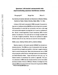
Sep 14, 2006 - manipulated by the gate voltages VgF , where EcF is the effective charging energy and ngF = VgF CgF /2e is the offset reduced gate charge of ...
Maxwell’s Demon Assisted Thermodynamic Cycle in Superconducting Quantum Circuits H.T. Quan,1, 2 Y.D. Wang,1, 2 Yu-xi Liu,1 C.P. Sun,1, 2 and Franco Nori1, 3
arXiv:quant-ph/0512063 v2 14 Sep 2006
1
Frontier Research System, The Institute of Physical and Chemical Research (RIKEN), Wako-shi, Saitama 351-0198, Japan 2 Institute of Theoretical Physics, Chinese Academy of Sciences, Beijing, 100080, China 3 Center for Theoretical Physics, Physics Department, CSCS, The University of Michigan, Ann Arbor, Michigan 48109-1040 (Dated: September 15, 2006) We study a new quantum heat engine (QHE), which is assisted by a Maxwell’s demon. The QHE requires three steps: thermalization, quantum measurement, and quantum feedback controlled by the Maxwell demon. We derive the positive-work condition and operation efficiency of this composite QHE. Using controllable superconducting quantum circuits as an example, we show how to construct our QHE. The essential role of the demon is explicitly demonstrated in this macroscopic QHE. PACS numbers: 05.30.-d, 03.67.-a, 85.25.Cp
Introduction.— A Maxwell demon is a construct that can distinguish the velocities of individual gas molecules and then separate hot and cold molecules into two domains of a container, so that the two domains will have different temperatures [1]. This result seems to contradict the second law of thermodynamics, because one can put a heat engine between them to extract work. The solution of this puzzle [1] refers to the so-called Landauer’s principle [2, 3] that essentially links information theory with fundamental physics [4]. Several quantum heat engines (QHEs) assisted by Maxwell’s demons have been proposed in Refs. [5, 6, 7]. Here, we propose a new QHE model integrated with a built-in quantum Maxwell’s demon performing both: the quantum measurement on the working substance, and the feedback control for the system according to the measurement. We demonstrate the role of Maxwell’s demon in a fully quantum manner. The thermodynamic cycle in our setup contains three fundamental stages: (i) a CNOT operation, making a pre-measurement to extract information from the working substance; (ii) the feedbackaction of the demon controlling the working substance to extract work; and (iii) the disentanglement process that thermalizes the working substance and the demon by two separate thermal baths. The demon plays a role in the first two steps. We further illustrate how to implement our QHE using superconducting qubit circuits [8, 9]. In our setup, the demon-assisted working substance does work via two CNOT operations, which can be realized by single-qubit operations and an easily realized i-SWAP operation. The CNOT operation performs the basic functions of the quantum demon. Maxwell’s demon-assisted thermodynamic cycle in twoqubit system.— Our QHE cycle is similar to a quantum Otto cycle [10] described in Ref. [11] and generalized in Ref. [12]. Here, the QHE, shown in Fig. 1, is a composite system consisting of two qubits: the “working substance” S and the quantum Maxwell’s demon D. They
System’s bath (TS)
Qin 1 0
S
∆S
W
S
S
c
D Demon’s bath (TD)
∆D
1 0
D D
Qout
FIG. 1: (color online). Schematics of the Maxwell’s-demonbased quantum heat engine (QHE). The qubit S is the “working substance” system, which is monitored and then controlled by another qubit D, acting as a Maxwell’s demon. The central circle with the letter “c” denotes a switchable coupling between the S and the D. S plus D form the QHE. Qin and Qout indicate the heat absorbed and released; W denotes the work done. When the erasure of D is included in the cycle, according to Landauer’s principle, the violation of the Second Law is prevented.
are separately coupled to two different heat baths with the temperatures TS and TD . Using the Pauli matrices (F ) σα (F = S, D; α = x, y, z), the model Hamiltonian can be written as X HI = ∆F σz(F ) + EL (σx(S) σx(D) − σy(S) σy(D) ), (1) F =S,D
where ∆F is the level spacing of the qubits and EL is a controllable coupling strength between S and D. Using both the controllable XY interaction and on-site potentials in Eq. (1), we can realize various quantum logic operations [13]. Now, let us study each step of our QHE cycle and calculate the work done and the heat absorbed in each step of the thermodynamic cycle. S1 : S and D are decoupled by setting EL = 0 in Eq. (1) and separately coupled to two heat baths
2 with different temperatures TS and TD . As shown below, whatever are the initial states of S and D, either entangled or separated, after a thermalization, they will reach their respective equilibrium states: ρF (1) = pF (0)|0F ih0F | + pF (1)|1F ih1F |, with F = S or D. Here, pF (1) = exp(−βF ∆F )/zF , and pF (0) = 1/zF , are the Boltzmann probability distributions for two energy levels; zF = 1 + exp(−βF ∆F ) is the partition function with βF = 1/(kB TF ), where kB is the Boltzmann constant. We have chosen the ground state energy as zero. The thermalized state ρ(1) = ρS (1) ⊗ ρD (1) of the total system is 1,1 1,0 ρ(1) = pS,D |1, 1ih1, 1| + pS,D |1, 0ih1, 0|
(2)
0,1 0,0 + pS,D |0, 1ih0, 1| + pS,D |0, 0ih0, 0|,
where for F, F ′ = S, D and q, q ′ = 0, 1, |q, q ′ i ≡ ′ ′ ′ |qS i ⊗ |qD i and pq,q F,F ′ ≡ pF (q) pF ′ (q ) being the joint probabilities. S2 : The second step is a CNOT operation flipping the demon states only when the working substance system is in its excited state [6]. In this step, the demon acquires information about the system. This CNOT process can be realized [13] by the controllable Hamiltonian (1) and is assumed to be so short that the coupling of S and D to the baths can be ignored. Thus, ρ(1), after the second step, is changed to 1,1 1,0 ρ(2) = pS,D |1, 0ih1, 0| + pS,D |1, 1ih1, 1|
(3)
0,0 0,1 |0, 0ih0, 0|. |0, 1ih0, 1| + pS,D +pS,D
The entropy of ρ(2) is equal to that of ρ(1), i.e., measurements do not lead to entropy increase [2, 3, 5]. This agrees well with Landauer’s principle. S3 : In the third step, the demon controls the system to do work according to the information acquired by the demon about the system. Physically, the system experiences a conditional evolution (CEV) Uc which can be ′ realized by the Hamiltonian (1), that is, |qS i ⊗ |qD i→ � ′ q ′ ˜ (Uc ) |qS i ⊗ |qD i and Uc |qS i = |˜ qS i. Here, 1S = � cos θ |1S i + sin θ exp(iϕ) |0S i, and ˜ 0S = − sin θ |1S i + cos θ exp(iϕ) |0S i, are the states of the working substance after the conditional evolution; θ and ϕ are real parameters. A CNOT is a special CEV for θ = π/2. After the third step, the density matrix ρ(2) evolves into 1,1 1,0 ˜ � ˜ 1, 1 1, 1 (4) ρ(3) = pS,D |1, 0i h1, 0| + pS,D �
0,1 ˜ 0,0 +pS,D 0, 1 ˜ 0, 1 + pS,D |0, 0i h0, 0| .
Finally, the system and the demon are decoupled by setting EL = 0 in Eq. (1) and brought into contact with their own baths again, and then a new cycle starts. For each cycle described above, we are now able to calculate the work performed by the heat engine as W = 2 1,0 1,0 ˜ ′′ − (ES′′ + ED − ES − ED ) = ∆S (pS,D − pS,D 1 |1i −
1,1 1,0 ′′ ′′ ˜ 2 p0,1 S,D 0 |1i )+∆D (pS,D −pS,D ), where ES (ES ) and ED (ED ) are the internal energies of the system and demon, respectively, after the third (first) step. The heat absorbed by the system from the heat bath is Qin = ES −ES′′ 2 0,1
1,0 ˜ ˜ 2 = ∆S (p1,0 S,D −pS,D 1 |1i −pS,D 0 |1i ). Based on the above results, the operation efficiency η can be given as η = W/Qin = 1 − (∆D /∆S )ξ
(5)
with � �� �−1 1,0 0,1 1,0 ξ = csc2 θ p1,1 /p − 1 p /p − 1 . S,D S,D S,D S,D
(6)
Equation (5) shows that ξ ≥ 0 (to guarantee the operation efficiency η < 1). The first factor of ξ in Eq. (6) is positive, while the second factor, which can be simplified to exp(−βD ∆D ) − 1, is negative. Thus, we can conclude that the third factor of ξ in Eq. (6) is negative. This results in TS ≥ TD (∆S /∆D ), and it agrees well with the positive-work condition [11, 12] for a simple quantum Otto cycle without Maxwell’s demon. This coincidence is nontrivial since here TS and TD are the temperatures of the baths surrounding qubits S and D in the whole cycle. This is different from the temperatures in Refs. [11, 12], where the two temperatures are defined by two different isochoric steps in thermodynamic cycles. Remarks on the QHE cycle and the roles of the quantum Maxwell’s demon.— Let us further understand each step in the above QHE operations. We first consider the thermalization problems for the two qubits coupled to two separated baths, which can be modelled as two collections of harmonic oscillators with different temperatures, e.g., TS and TD . The baths have the average thermal excitation n(TF , ωF ) = 1/[exp(βF ωF ) − 1] in the mode with frequency ωF (F = S, D) of the baths. After thermalization, the population difference of F can be calculated [16] as hσz(F ) (t)i =
� 1 � (F ) hσz (0)iMF + 1 e−2γF t −(1/MF ) , (7) 2
where MF = 1 + 2 n(TF , ∆F ) is time-independent. The damping rate γF of F depends on the specific physical realization. When t ≫ 1/γF , F will approach its (F ) steady state ρF (1) in Eq. (2) with hσz (t → ∞)is = −1/MF . Then, we can obtain the equilibrium distribution, pF (1) = (1 − 1/MF )/2, of the two-level system, (F ) using pF (1) ± pF (0) = hσz (t)i(1∓1)/2 . It is crucial that (F ) the steady term hσz (t → ∞)is in Eq. (7) is independent of the initial state, since the initial information is erased by quantum dissipation, with damping rate γF . Hence, whatever initial state the total system is (e.g., an entangled state), the final steady state of S or D would be in its own thermal equilibrium state. The CNOT operation in the step S2 can be referred to a one-bit quantum pre-measurement on the quantum
3 (a)
⊗
CgS
L
⊗
S
⊗
CgD
D
VgS
VgD
(b) π 2 Z
π 2 X
X
π 2
X
π 2
Z
X
S i–SwAP
π 2
i–SwAP
Z
i–SwAP
π − 2
π 2
i–SwAP
system S by the Maxwell’s demon [5]. As for the CEV in step S3, we noticed that, when we choose i) the CEV to be a special case θ = π/2, i.e., a CNOT, and ii) the temperature TD to be so low that exp(−βD ∆D ) ≪ 1, i.e., the demon is “erased” nearly to its ground state ρD (1) ≈ |0D i h0D | [15], the efficiency of our QHE Eq. (5) becomes η = 1 − (∆D /∆S ). This is exactly the efficiency of a simple quantum Otto cycle without Maxwell’s demon [10, 11, 12]. Otherwise the operation efficiency (5) is less than the efficiency of a simple quantum Otto cycle. This is because i) when TD is vanishingly small, the demon can be restored to a zero-entropy “standard state” [3, 15] to acquire information about the system in the most efficient way, and ii) among all CEVs the CNOT is the optimum operation to extract work. One might ignore the effect of the demon by only considering the reduced density matrix ρS = TrD [ρ] of S by tracing over the variable of D. After the step S3, one has the reduced density matrix ρS (3) = TrD [ρ(3)]. The following thermalization of ρS (3) restores S into its initial equilibrium state ρS (1) by absorbing heat. Therefore, the net result of ignoring the demon means that there exists a perpetual machine of the second kind, which absorbs heat from a single heat bath and converts it into work. This obvious violation of the second law of thermodynamics leads to the so-called “Maxwell’s demon paradox”. When the demon is included in the thermodynamic cycle, however, the “paradox” disappears and the violation of the second law is prevented. Hence the present concrete model shows the effect of Maxwell’s demon and verifies the prediction of Landauer’s principle. Experimental implementation based on superconducting systems.— The above Maxwell’s demon assisted QHE model can be demonstrated by a realistic system, e.g., the superconducting quantum circuit illustrated in Fig. 2(a), described by the Hamiltonian (1). Here, two qubits S and D are specified to two charge qubits [8] with the controllable level spacings ∆F = EcF |ngF − 1/2| (F = S, D), manipulated by the gate voltages VgF , where EcF is the effective charging energy and ngF = VgF CgF /2e is the offset reduced gate charge of the qubit F . Here, the magnetic fluxes threading the two qubits are set to Φ0 /2. The coupling constant EL = E0 cos(πΦx /Φ0 ) can be tuned to zero by the external magnetic flux Φx through the dc SQUID L, where E0 is the Josephson tunnelling energy. Therefore, the inter-qubit coupling can be switched on and off by the magnetic flux Φx . Below We explain how to implement our QHE by using the circuit in Fig. 2(a). To implement the step S1 in our proposal, we turn off the interaction between two qubits by applying the magnetic flux Φx = Φ0 /2. The two charge qubits are coupled to their own baths, which can be realized by two local temperatures TS and TD . This temperature difference can be guaranteed by temperature gradient. Thus, with a thermalization time of about 1 ∼ 10 µs [17], two superconducting charge qubits can reach their own
π 2
Z
D
FIG. 2: (color online). A Maxwell’s demon QHE implemented by a superconducting circuit. (a) two charge qubits S and D with different localized temperatures function as the working substance and the demon, respectively. VgF and CgF are the gate voltage and capacitance of qubit F . (b) The quantum logic operations (two CNOTs) to simulate the demon are realized by four i-SWAP operations together with several single-bit operations [13], e.g., [Θ]X , a Θ-rotation along the x axis. Here Θ = ±π/2. The quantum control to implement these operations is carried out by the dc SQUID L in (a).
equilibrium states, described by Eq. (2). The population of each qubit is described by the steady term of Eq. (7). After two qubits reach their equilibrium states, the step S2 starts to implement a CNOT operation with the demon being the target qubit, and the working substance being the controlling qubit. This CNOT can be obtained [13] as follows: First, two single-qubit operations, [π/2]X and [π/2]Z , are applied on the system as well as one single-qubit operation, [−π/2]Z , on the demon, here [Θ]i (i = X, Z) denotes a Θ-rotation along the i axis. Second, we turn on the two-qubit interaction by setting Φx = 0 and ngS ≈ ngD ≈ 1/2. Then, two coupled qubits evolve in time t0 = π~/(4E0 ) (about 1 ∼ 10 ns [8]) through the Hamiltonian (1) to get an i-SWAP operation. Third, turn off the two-qubit interaction, and a [π/2]X operation is only applied to the demon. Fourth, the two-qubit interaction is turn on again and the two qubits evolve t0 = π~/(4E0 ). Finally, switch off the twoqubit interaction, and a [π/2]Z operation is applied to the system. After these steps, a CNOT operation is implemented on the two qubits by the quantum circuit in Fig. 2(a) and Eq. (3) is obtained. We now consider the step S3. In our proposed experimental setup in Fig. 2(a), the CEV operation in the step S3 is chosen as a CNOT operation, with the demon being the controlling qubit, and the working substance being the target qubit. This CNOT can be obtained similarly
4 as the step S2. In this case, the work done by the QHE is maximum, since the demon flips the system from the excited state |1iS to the ground state |0iS . After the step S3, the qubit interaction is switched off by Φx = Φ0 /2, then our QHE starts a new cycle. The two CNOT operations used in S2 and S3 are schematically shown in Fig. 2(b). The total time for these two operations in the charge-qubit circuits [8] is ∼ 10 ns, which is much less than the relaxation time 1 ∼ 10 µs [17]. In the above quantum circuits, if the temperature TD is so low that exp(−βD ∆D ) ≪ 1, the efficiency η in Eq. (5) of our proposed QHE approaches η = 1 − ∆D /∆S of a simple quantum Otto heat engine [10, 11, 12]. In the experimental setup, the parameters usually are of the following order of the magnitude [18]: EcS ∼ 10−23 J, |2ngS − 1| ∼ 10−2 , TS ∼ 10−2 K. Hence, exp(−βS ∆S ) ∼ e−1 . If we choose EcS ∼ EcD and TD ∼ (TS /10) ∼ 10−3 K, then we certainly have exp(−βD ∆D ) ∼ e−10 ≪ 1. Using the parameters about ∆D and ∆S of the superconducting qubits, the efficiency η of the QHE can be further given by η =1−
|2ngD − 1| , |2ngS − 1|
(8)
which is independent of TS and TD . Here, we have adjusted the macroscopic quantum circuit to be symmetric with respect to D and S by choosing EcS = EcD . For instance, if ngD = 0.498 and ngS = 0.492, the efficiency becomes η = 0.75. The derived expression, in Eq. (8), for the QHE efficiency could be tested by experiments on superconducting qubit circuits. There are three important conditions for the experimental implementation of our QHE: i) controllable two-qubit operations; ii) two different temperatures TS and TD for the two nearby qubits; and iii) precise measurements of the power of the microwave irradiations. The first one has been discussed above. The second condition could be achieved by a temperature gradient on the chip. For the third condition, a precise measurement of the power spectrum of the microwave is experimentally accessible in these circuits. Hence, the heat Qin absorbed by S and the heat Qout released by D can be measured, when they are in contact with their respective baths in the step S1. Similar to the arguments in Ref. [6, 7, 11, 12], the work produced in this cycle depends on the conservation of energy W = Qin − Qout and does not depend on the specific operation performed. We can also estimate the output power of the QHE. From Eqs. (5) and (8), we have W ∼ ηQin ∼ η ∆S pS (1) ∼ 10−25 J, and the time interval of a cycle is about τ ∼ 10 µs. Hence the output power becomes P = W/τ ∼ 10−20 J s−1 . We emphasize that we are now interested in conceptual designs of new types of QHEs, rather than their engineering applications. In summary, we have studied the operation of a Maxwell’s-demon-assisted QHE and justified the predic-
tions of Landauer’s principle: i) a measurement does not necessarily lead to entropy increase [2, 3, 5]; and ii) the apparent violation of the second law does not hold when the restoration of the demon’s memory is included in the cycle [1, 2, 3, 4, 5, 6, 7], because under certain conditions, our composite QHE is equivalent to a simple quantum Otto engine. We also use superconducting quantum circuits as an example showing how to implement this QHE. FN is supported in part by NSA, LPS, ARO, and NSF. CPS is partially supported by the NSFC and NFRP of China.
[1] H.S. Leff and A.F. Rex (eds.), Maxwell’s Demon 2: Entropy, Classical and Quantum Information, Computing (Bristol, Institute of Physics, 2003). [2] R. Landauer, IBM J. Res. Dev. 5, 183 (1961). [3] See, e.g., C.H. Bennett, Int. J. Theor. Phys. 21, 905 (1982); Sci. Am. 257, 108 (1987). [4] K. Maruyama et al., J. Phys. A 38, 7175 (2005). [5] W.H. Zurek, arXiv: quant-ph/0301076. [6] S. Lloyd, Phys. Rev. A 56, 3374 (1997). [7] M.O. Scully Phys. Rev. Lett. 87, 220601 (2001); M. O. Scully et al., Physica E 29, 29 (2005); Y. Rostovtsev et al., ibid. 29, 40 (2005); Z. E. Sariyanni et al.,ibid. 29, 47 (2005). [8] Y.D. Wang et al., Phys. Rev. B 72, 172507 (2005). [9] Y.X. Liu et al., Phys. Rev. Lett. 96, 067003 (2006). [10] For an Otto type QHE [11, 12] using a potential well (e.g., an infinite square or a harmonic oscillator), the efficieny of the Otto cycle (two isochoric and two adiabatic processes) is 1 − ∆2 /∆1 , where the level-spacing ∆1 (∆2 ) of the first (second) isochoric process is determinded by the width of the potential well. Each isochoric process implies that the level spacing is constant. In our model, the thermalization processes (step 1) play the role of the isochoric processes. The efficiency and positive-work condition of our model becomes that of known engines in [11, 12] under certain conditions. We also noticed the inconsistency in defining Otto type QHE, see e.g., Ref. [14], which do not affect the main idea of our paper. [11] T.D. Kieu, Phys. Rev. Lett. 93, 140403 (2004); Eur. J. Phys. D 39, 115 (2006); E. Geva and R. Kosloff, J. Chem. Phys. 96, 3054 (1992); J. Arnaud, L. Chusseau, F. Philippe, quant-ph/0211072. [12] H.T. Quan et al., Phys. Rev. E 72, 056110 (2005). [13] N. Schuch and J. Siewert, Phys. Rev. A 67, 032301 (2003). [14] M.O. Scully, Phys. Rev. Lett. 88, 050602 (2002); Y.V. Rostovtsev et al., Phys. Rev. A 67, 053811 (2003); M.O. Scully et al., Science 299, 862 (2003); T. Opatrny, et al., Fortschr. Phys. 50, 657 (2002); A.E. Allahverdyan, T. Nieuwenhuizen, Phys. Rev. E 71, 046106 (2005). [15] M.B. Plenio and V. Vitelli, Contemp. Phys. 42, 25 (2001); E. Lubkin, Int. J. Theor. Phys. 26, 523 (1987); V. Vedral, Pro. R. Soc. Lond. A 456, 969 (2000). [16] M. Orszag, Quantum Optics (Berlin, Springer, 1999). [17] J.Q. You and F. Nori, Phys. Today 58, No. 11, 42 (2005). [18] Y. Nakamura, Y. Pashkin, J. Tsai, Nature 398, 786
5 (1999).