Quantum mechanics of null polygonal Wilson loops

Quantum mechanics of null polygonal Wilson loops

arXiv:1401.7307v1 [hep-th] 28 Jan 2014

A.V. Belitskya , S.E. Derkachovb , A.N Manashovc,d a

b

St. Petersburg Department of Steklov Mathematical Institute Fontanka 27, 191023 St. Petersburg, Russia c

d

Department of Physics, Arizona State University Tempe, AZ 85287-1504, USA

Institut f¨ ur Theoretische Physik, Universit¨at Regensburg D-93040 Regensburg, Germany

Department of Theoretical Physics, St.-Petersburg State University 199034, St.-Petersburg, Russia

Abstract Scattering amplitudes in maximally supersymmetric gauge theory are dual to super-Wilson loops on null polygonal contours. The operator product expansion for the latter revealed that their dynamics is governed by the evolution of multiparticle GKP excitations. They were shown to emerge from the spectral problem of an underlying open spin chain. In this work we solve this model with the help of the Baxter Q-operator and Sklyanin’s Separation of Variables methods. We provide an explicit construction for eigenfunctions and eigenvalues of GKP excitations. We demonstrate how the former define the so-called multiparticle hexagon transitions in super-Wison loops and prove their factorized form suggested earlier.

Contents 1 Motivation 1.1 Soft-collinear expansion of polygons . . . . . . . . . . . . . . . . . . . . . . . . . . . . . 1.2 Light-cone operators . . . . . . . . . . . . . . . . . . . . . . . . . . . . . . . . . . . . . .

2 3 5

2 Open spin chain 2.1 Scalar product . . . . . . . . . . . . . . . . . . . . . . . . . . . . . . . . . . . . . . . . . 2.2 Integrals of motion . . . . . . . . . . . . . . . . . . . . . . . . . . . . . . . . . . . . . . .

8 9 10

3 Factorized R-matrices and Hamiltonians 3.1 Intertwiners . . . . . . . . . . . . . . . . . . . . . . . . . . . . . . . . . . . . . . . . . . . 3.2 Hamiltonians . . . . . . . . . . . . . . . . . . . . . . . . . . . . . . . . . . . . . . . . . .

11 11 13

4 Baxter operators and Baxter equations 4.1 Baxter operator Q+ . . . . . . . . . . . 4.2 Baxter operator Q− . . . . . . . . . . . 4.3 Baxter equations . . . . . . . . . . . . . 4.4 Hamiltonians from Baxter operators . .

. . . .

14 14 16 17 18

5 Eigenfunctions 5.1 Recurrence relation . . . . . . . . . . . . . . . . . . . . . . . . . . . . . . . . . . . . . . . 5.2 Integral representation of eigenfunctions . . . . . . . . . . . . . . . . . . . . . . . . . . . 5.3 Proof of orthogonality . . . . . . . . . . . . . . . . . . . . . . . . . . . . . . . . . . . . .

19 19 20 23

6 Scalar product on real line 6.1 Relation between scalar products . . . . . . . . . . . . . . . . . . . . . . . . . . . . . . .

25 26

7 Multiparticle transitions 7.1 Square transitions . . . . . . . . . . . . . . . . . . . . . . . . . . . . . . . . . . . . . . . 7.2 Hexagon transitions . . . . . . . . . . . . . . . . . . . . . . . . . . . . . . . . . . . . . .

28 29 30

8 Conclusions

33

A Parametrization of polygons A.1 Coordinates ↔ twistors . . . . . . . . . . . . . . . . . . . . . . . . . . . . . . . . . . . . A.2 Reference square . . . . . . . . . . . . . . . . . . . . . . . . . . . . . . . . . . . . . . . . A.3 Octagon and decagon . . . . . . . . . . . . . . . . . . . . . . . . . . . . . . . . . . . . .

33 34 35 37

B Feynman graphs

38

C Intertwining relations C.1 Intertwining relation (6.2) . . . . . . . . . . . . . . . . . . . . . . . . . . . . . . . . . . . C.2 Formula (6.13) . . . . . . . . . . . . . . . . . . . . . . . . . . . . . . . . . . . . . . . . .

40 40 42

D Separation of Variables D.1 Diagonalization of BN . . . . . . . . . . . . . . . . . . . . . . . . . . . . . . . . . . . . . D.2 Transformation to SoV . . . . . . . . . . . . . . . . . . . . . . . . . . . . . . . . . . . . .

44 44 45

. . . .

1

. . . .

. . . .

. . . .

. . . .

. . . .

. . . .

. . . .

. . . .

. . . .

. . . .

. . . .

. . . .

. . . .

. . . .

. . . .

. . . .

. . . .

. . . .

. . . .

. . . .

. . . .

. . . .

. . . .

. . . .

. . . .

1

Motivation

Recently, it was suggested that null polygonal super-Wilson loop may serve as a generating function for all scattering amplitudes in (regularized) planar maximally supersymmetric SU (N ) Yang-Mills theory. The equivalence was first established for the so-called Maximally Helicity Violating (MHV) gluon amplitudes, that involve two particles with helicities opposite to the rest, and the holonomy of a gauge connection circulating around a closed contour composed of straight light-like segments [1, 2, 3]. These segments are identified with momenta of incoming gluons involved in the scattering process and one regards the resulting loop as living in a dual coordinates space [4, 2]. The conventional soft and collinear divergences of massless gluon amplitudes emerge in this picture from the ultraviolet singularities stemming from virtual corrections in the vicinity of the cusps where the two adjacent segments meet in a point. However, not only the divergent parts were shown to agree, but also finite contributions to both coincide as well. By uplifting the contour to superspace, the duality establishes the equivalence1 between the vacuum expectation bn value of the super-Wilson loop Wn in N = 4 SYM and the reduced N -particle matrix element A of the S-matrix of the theory [5, 6] that is expected to hold nonperturbatively in ’t Hooft coupling 2 Nc /(4π 2 ). The former is determined by bosonic Aαα˙ and fermionic FαA connections a = gYM    Z Z igYM 1 αα ˙ αA dx Aαα˙ + igYM dθ FαA tr P exp , (1.1) hWn (xi , θi ; a)i = Nc 2 Cn Cn that live on a piece-wise contour in superspace Cn = [X1 , X2 ] ∪ [X2 , X3 ] ∪ · · · ∪ [Xn , X1 ] with cusps located at superpoints Xi = (xi , θi ). Both superfields Aαα˙ and FαA receive a terminating series in the Grassmann variable θ, with their expansion coefficients being determined by the field content of the N = 4 SYM (see, e.g., Ref. [7] for details). The dynamical content of the duality is summarized by the following equation bn (Zi ; a) , hWn (Xi ; a)i = A

(1.2)

where the right-hand side corresponds to the reduced n-particle S-matrix element upon extraction of the conservation laws for the supermomentum (pαα˙ , qαA ) Sn = i(2π)4

δ (4) (pαα˙ )δ (8) (qαA ) b An (Zi ; a) . h12ih23i . . . hn − 1ni

(1.3)

The kinematical variables entering the super-Wilson loop are related to the momentum superb 2 twistors ZiA = (λαi , µiα˙ , χA i ) defining the superscattering amplitude via the relation Xi = Zi−i ∧ Zi .

(1.4)

In addition to the conservation-law delta functions, we traditionally factored out the denominator of the Parke-Taylor tree amplitude [10], where the angle brackets between bosonic twistors are conventionally defined as hiji = λαi λjα . A brute force calculation of the super-Wilson loop represents a challenge on its own even at lowest orders in coupling a, thus exposing inefficiency of usual techniques based of Feynman diagrams. It was noticed however that the left-hand 1

A proper care has to be taken to handle the regularization of ultraviolet divergences [7] in order to maintain supersymmetry of the super-loop and conformal symmetry of the so-called remainder function [8, 9]. 2 A brief summary of our conventions is summarized in Appendix A.1.

2

side of the above relation (1.2) is advantageous in computing the S-matrix since the Wilson loop formalism allows one to break free from limitations of perturbation theory, being more amenable to nonperturbative techniques [1]. Such a techniques was put forward a little while ago and is based on the operator product expansion (OPE) [11]. Recently, a complementary view on this framework was offered by exhibiting its connection to the expansion in terms of light-cone operators with boundary fields set by light-like Wilson lines, or the Π-shaped Wilson loop with field insertions [12, 13]. The renormalization group evolution of the latter was shown to be governed by a noncompact open spin chain [12], whose eigenenergies provide corrections to leading discontinuities of the Wilson loop, while the corresponding eigenfunctions define the coupling of the Gubser-Klebanov-Polyakov (GKP) excitations [14, 15] to the Wilson loop contour as well as their multiparticle transition amplitudes. In this paper we explore the emerging open spin chain. We will focus on the component formalism leaving a fully supersymmetric superspace formulation for future publication. Notice that quite recently a framework that combines the OPE and integrability was proposed in Ref. [16]. It is based on a few conjectured equations obeyed by building blocks of the Wilson loops that are matched to explicit calculations of amplitudes and bootstrapped to all orders in ’t Hooft coupling. The next section follows a similar construction.

1.1

Soft-collinear expansion of polygons

To start with, let us recall the emergence of non-local light-cone operators in the OPE of the super-Wilson loop. We will discuss it in a simplified set-up of restricted kinematics [17], i.e., when the bosonic part of the Wilson loop contour is embedded in a two-dimensional plane3 . The first nontrivial Wilson loop in this kinematics is the octagon. Let us focus on NMHV amplitudes and choose a specific Grassmann component that admits a clear OPE interpretation, say χ2 χ3 χ6 χ7 . It was calculated diagrammatically in Ref. [18] and also making use of the so¯ called Q-equation in Ref. [19]. The subtracted superloop, with ultraviolet divergences eliminated in a superconformally invariant fashion, reads to two loop accuracy  
χ2 χ3 χ5 χ6 2 R + + − − + − 3 a + a ln u (1 + u ) ln u (1 + u ) − 2 ln(1 + u ) ln(1 + u ) + O(a ) , hW8 i = h2367i (1.5) where the conformal cross ratios are u+ =

+ x+ 34 x78 + , x+ 37 x48

u− =

− x− 23 x67 − . x− 26 x37

(1.6)

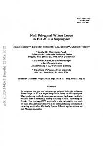
The leading contribution in the OPE of this channel stems from the scalar exchange between the cusps at points x3 and x4 , see Fig. 1 (a). The soft-collinear expansion corresponds to the limit + x+ 32 → 0 and x67 → 0, which results in flattening of the octagon to a square, see Appendix A.2. The subleading perturbative corrections come from a number of Feynman graphs encoding the interaction of the scalar field with the contour, Fig. 1 (b), vertex corrections and independent propagation of a gauge field along with the original scalar, Fig. 1 (c). A natural set of the cusp coordinates, or equivalently twistors, to discuss the OPE is introduced in Appendix A.3. In this 3

To preserve superconformal symmetry this implies that out of four components of the Grassmann χA two of them have to vanish as well. However, this subtlety is not relevant for our present discussion and we will assume that all components of χA i are nonzero at even and odd sites.

3

frame, the remainder function admits the form hW8R i =


 χ2 χ3 χ5 χ6  a + a2 τ ln(1 + e2σ )(1 + e−2σ ) + ln(1 + e−2τ )(1 + e2σ ) + O(a3 ) . 4 cosh τ cosh σ

The afore-introduced soft-collinear asymptotics translates into the τ → ∞ limit, with the remainder function corresponding to a single scalar GKP excitation (also known as a hole) propagating in the OPE channel4 Z ∞ R τ →∞ hW8 i = χ2 χ3 χ5 χ6 du µh (u; a) exp (−τ Eh (u; a) − iσ ph (u; a)) + O(e−3τ ) . (1.7) −∞

Here the energy and momentum of the hole excitation read to one-loop accuracy [14, 15]   Eh (u; a) = 1 − a 2ψ(1) − ψ( 12 + iu) − ψ( 21 − iu) + O(a2 ) , (1.8) 2 ph (u; a) = 2u − 2πa tanh(πu) + O(a ), (1.9) while the measure encoding the coupling of the excitation to the Wilson loop contour is     2 π 3 2 2 µh (u; a) = µh (u) a + a π 1 − . (1.10) + O(a ) , µh (u) = 2 cosh(πu) cosh (πu) In this equation, the O(a2 ) term is merely needed to compensate the O(a2 ) correction to the momentum (1.8) to match the OPE expansion into the exact two-loop data (1.7). By expanding the right-hand side to next-to-leading order in a, we immediately reproduce the τ -enhanced contribution in Eq. (1.7). A similar consideration can be performed for the decagon. Using the conformal frames discussed in Appendix A.3, we can write the remainder function of the χ2 χ3 χ8 χ9 NMHV component [19] of the super-Wilson loop in the form 1 χ2 χ3 χ8 χ9 (1.11) 4 cosh(τ1 − τ2 ) 2 cosh(σ1 − σ2 ) + e−σ1 −σ2   (2 cosh(σ1 − σ2 ) + e−σ1 −σ2 )2 (2 cosh(σ1 − σ2 ) + e−σ1 −σ2 )2 2 × a + a 2τ1 ln + 2τ ln 2 1 + e−2σ2 1 + e−2σ1 1 + e−2σ1 − ln(1 + e−2τ2 ) ln(1 + e−2σ1 )(1 + e−2σ2 ) + ln(1 + e−2τ1 ) ln 1 + e−2σ2 

R hW10 i=

+ 2 ln(1 + e−2τ1 −2τ2 ) ln(1 + e−2σ2 + e2σ1 −2σ2 )

.

As above, the leading asymptotic is governed by a single hole excitation Z ∞ R τ1,2 →∞ hW10 i = χ2 χ3 χ8 χ9 du dv µh (u; a)Hh (u|v; a)µh (v; a) −∞

× exp (−τ1 Eh (u; a) − τ2 Eh (v; a) − iσ1 ph (u; a) − iσ2 ph (v; a)) + O(e−3τ1,2 ) , where the hexagon transition kernel reads to this order in coupling   Hh (u|v; a) = Hh (u|v) a−1 + 2ψ 0 ( 12 + iu) + 2ψ 0 ( 21 − iv) − π 2 + O(a) , 4

Notice that our definition of the rapidity variable differs by a sign from the conventions of Ref. [16].

4

(1.12)

(1.13)

+− ⊗ F

x6

x8 x7

x+

x−

x5 ε

x−

x+

x−

x+

.

x1 ε −1

−1

ε −1

ε −1

x3 x4

(a)

.

x2

0

(b)

0

0

0

(c)

F +− 0

⊗ 0

Figure 1: Single (a,b) and two-particle (c) contributions to OPE of the octagon. The one-loop graph in (a) given by the scalar propagator exchanged between the cusps produces a components of the tree NHMV amplitude. The graph in panel (b) displays one of the perturbative corrections due to the Hamiltonian acting on the light-cone operator. In (c) we show the two-particle contribution that produces subleading effects in the OPE. with the leading term being Hh (u|v) =

Γ( 12

Γ(iv − iu) . + iv)Γ( 12 − iu)

(1.14)

As we recall in the next section, these leading contributions in the asymptotic expansion, i.e., O(e−τ1,2 ), come from the renormalization of a nonlocal operator with a Π-shaped contour, formed by two Wilson lines building up the contour in a given OPE channel and an elementary scalar field insertion, while the subleading effects correspond to more than one GKP excitations sandwiched between the boundary Wilson lines.

1.2

Light-cone operators

Let us cast the above heuristic discussion into an operator language. We will do it for the octagon at two-loop order and then generalize it to an arbitrary number of GKP excitations exchanged in a given OPE channel. As one takes the limit τ → ∞, the top and bottom portions of the contour of the octagon Wilson loop get flatten out and one ends up with a scalar field Z inserted into the top and bottom straight-line segments. Each of these correspond to a Π-shaped light-cone operator of the form Oh (x) = W † (0)[0, x+ ]− Z(x+ )[x+ , ∞]− W (∞) ,

(1.15)

where the boundary fields W (x+ ) stand for the Wilson lines stretched along the light-like direction x− starting at 0 and going to the null infinity 1/ε → ∞, localized at the position x+ on the tangent light-cone,   Z ∞ + − + + − W (x ) = P exp igYM dx A (x , x , 0⊥ ) . (1.16) 0

5

By a suitable gauge choice, i.e., the light-cone gauge A− = 0, one can even eliminate the gauge links between the fields in the composite operator, i.e., [. . . ]− → 1. The contribution of (1.15) to the the leading e−τ term in the OPE reads hW8R i =

aχ2 χ3 χ6 χ7 † hOh (x7 )(1 + aτ H1 )Oh (x3 )i . h23ih67i

(1.17)

For a = 0, this can be easily identified as a propagation of a free scalar from the bottom to the top of the loop, while the O(a) effect induces the τ -enhanced contribution to the two-loop remainder function and arises from the interaction of the scalar field with the Wilson loop contour by means of the light-cone Hamiltonian H1 = H01 + H1∞ ,

(1.18)

with individual Hamiltonians for the interaction with the left and right boundaries being [12] Z 1  dα  2s−1 α O(αx1 ) − O(x1 ) , (1.19) H01 O(x1 ) = 0 1−α Z ∞  dα  O(αx1 ) − α−1 O(x1 ) , (1.20) H1∞ O(x1 ) = α−1 1 respectively. Here we presented them in a generic form suitable for studies of elementary fields of conformal spin s. While for the case at hand, s = 1/2. For a one-particle GKP excitation, the diagonalization of the above Hamiltonian can be easily performed with a plane-wave eigenfunction 1 −s Ψu1 (x1 ) = x−iu , 1

(1.21)

that carries the momentum p(u1 ) = 2u1 and the energy H1 Ψu1 (x1 ) = [2ψ(1) − ψ(s + iu1 ) − ψ(s − iu1 )] Ψu (x1 ) ,

(1.22)

cf. Eq. (1.8). Analogously, we can perform the soft-collinear expansion for the decagon in terms of the light-cone operators (1.15). The formalism can be extended to account for multiparticle effects as well. As one collapses the top and bottom of the loop in the soft limit it gives rise to curvature corrections, actually an infinite series of them in increasing powers of the gluon field strength F +− . The first correction to the asymptotic behavior stems from the diagram shown in Fig. 1 (c) for the octagon. At even higher orders, the OPE involves multiparticle light-cone operators ON (x1 , . . . , xN ) = W † (0)[0, x1 ]X1 (x1 )[x1 , x2 ]X2 (x2 ) . . . XN (xN )[xN , ∞]W (∞) ,

(1.23)

where we stripped the + superscripts off the x-coordinates for brevity since it is the only component that will appear in the analysis that follows. Under renormalization group evolution, these operators mix and one has to solve the resulting eigensystem problem. In this work we will consider a simplified setup when all GKP excitations are of the same type Xn = X and possess a generic conformal spin s. The Hamiltonian HN = H01 +

N −1 X n=1

6

Hn,n+1 + HN ∞ ,

(1.24)

built-up from nearest-neighbor interactions only, in planar limit, is the one-loop dilatation operator acting on the operator (1.23) d ON (x1 , . . . , xN ) = −aHN ON (x1 , . . . , xN ) . d ln µ

(1.25)

Here the pair-wise Hamiltonians (including the boundary ones) can be encoded in a single formula Hn,n+1 ON (. . . , xn , xn+1 , . . . ) (1.26) " # 2s−1 Z 1 dα αxn+1 − xn = ON (. . . , xn , αxn+1 , . . . ) − ON (. . . , xn , xn+1 , . . . ) xn+1 − xn xn /xn+1 1 − α " # 2s−1 Z xn+1 /xn dα xn+1 − αxn 1 + ON (. . . , αxn , xn+1 , . . . ) − ON (. . . , xn , xn+1 , . . . ) . α−1 xn+1 − xn α 1 Their complementary representation in terms of differential operators reads H01 = ψ(1) − ψ(x1 ∂1 + 2s) , Hn,n+1 = 2ψ(1) − ψ(xn,n+1 ∂n + 2s) − ψ(xn+1,n ∂n+1 + 2s) − ln xn /xn+1 , HN ∞ = ψ(1) − ψ(−xN ∂N ) ,

(1.27)

where ψ(x) = d ln Γ(x)/dx is the Euler digamma function. It is important to notice that this is not the form naturally coming from the computation of Feynman graphs contributing to the renormalization of (1.23). Namely, the one-loop light-cone Hamiltonians for interaction of GKP excitations among themselves are not sensitive to the boundary Wilson lines and thus have to enjoy full SL(2, R) invariance [20, 21]. However, it is not the case in the above form due to the presence of the logarithms. The latter emerge from 1/α-factor in the second integral in Eq. (1.26) that was introduced in order to match it to the boundary Hamiltonians (1.19), with all intermediate logarithms canceling telescopically with one another. Therefore, in order to restore the conformal symmetry property, one can shift the logarithms into the boundary terms, such that the reshuffled Hamiltonians will become h01 = ψ(1) − ψ(x1 ∂1 + 2s) − ln x1 = − ln(x21 ∂1 + 2sx1 ) , hn,n+1 = 2ψ(1) − ψ(xn,n+1 ∂n + 2s) − ψ(xn+1,n ∂n+1 + 2s) , hN ∞ = ψ(1) − ψ(−xN ∂N ) + ln xN = − ln ∂N ,

(1.28)

PN −1 with HN = h01 + n=1 hn,n+1 + hN ∞ . Here we used identity (B.6) from Appendix B to recast the boundary Hamiltonians in terms of logarithms. At this point we would like to point out that similar Hamiltonians emerged in the discussion of the Regge limit of scattering amplitudes in Ref. [22]. Thus, the goal of this paper is to solve the spectral problem for the multiparticle Hamiltonian (1.24) HN Ψu (x1 , . . . , xN ) = Eu Ψu (x1 , . . . , xN ) .

(1.29)

The problem turns out to be integrable since the Hamiltonian HN possesses enough integrals of motion with eigenvalues u = (u1 , . . . , uN ) to be exactly solvable. Thus we have the powerful 7

machinery of integrable spin chain at our disposal for constructing the explicit eigenfunctions and finding the corresponding eigenvalues. For the case at hand we are dealing with an open spin chain that does not possess SL(2, R) symmetry due to boundary interactions. In addition, as we can conclude from the one-particle eigenfunction (1.21), the system is not endowed with a vacuum states. As a consequence of this last fact, the traditional methods based on the Algebraic Bethe Ansatz [23, 24] are not applicable and instead one has to rely on the method of the Baxter Q-operator [25] and the Separation of Variables (SoV) [26]. Our subsequent consideration is organized as follows. After introducing a natural Hilbert space for the Hamiltonian and a scalar product that makes it self-adjoint in the next section, we find a complete set of integrals motion commuting with HN . As a next step on the way to solve the spectral problem, we recall the factorization of R-matrices [23, 24] into intertwiners that play a crucial role in our construction. In Section 3, we use them to construct the Hamiltonians and demonstrate their equivalence with the ones arising in the problem of renormalization of the light-cone operators (1.23). Then in Section 4, we construct the Baxter Q-operator as well as its conjugate making use of available techniques developed for SL(2) invariant magnets. Both operators are then used to generate commuting Hamiltonians. In Section 5, we devise an iterative procedure to construct the eigenfunctions of the Hamiltonian. We then cast the latter in a form of a contour integral representation as well as an integral representation in the upper half-plane. The latter is instrumental in demonstration of their orthogonality under the scalar product introduced earlier. To adopt our construction for multiparticle contributions to the null polygonal Wilson loops, we define a new scalar product on the real half-line in Section 6 and establish its relation to the one for the analytically continued functions in the upper half-plane. Then we explicitly compute the square and hexagon transitions in Section 7, where we also prove the factorized ansatz for the latter suggested in Ref. [16]. Finally, we conclude by pointing applications of the current construction to the operator product expansion of polygonal Wilson loops and outline the generalization to include GKP excitations of different spins. Several appendices contain conventions and computational details that we found inappropriate to include in the main body of the paper as well as a complementary construction the wave function in the representation of Separated Variables and its relation to the eigenvalues of the Baxter Q-operator.

2

Open spin chain

The Hamiltonian (1.24) defines a non-periodic one-dimensional lattice model of interacting spins S n = (Sn0 , Sn+ , Sn− ) acting at each site defined by the coordinate of the GKP excitation. They form an infinite-dimensional representation of the sl(2, R) algebra, [Sn+ , Sn− ] = 2Sn0 ,

[Sn0 , Sn± ] = ±Sn± .

(2.1)

Our choice of the representation Sn±,0 for the spin generators S±,0 on the fields X is driven by the form of the pairwise Hamiltonians (1.28) acting on the elementary fields X(x), i.e. [S±,0 , X(xn )] = iSn±,0 X(xn ) [20, 21]. They are taken in the form of differential operators acting on lattice sites Sn+ = x2n ∂n + 2sxn ,

Sn− = −∂n ,

Sn0 = xn ∂n + s ,

(2.2)

where all labels of the representation s are the same for any n. The latter condition defines a homogeneous open spin chain. The spin variable s is assumed to be real and bounded from below by 1/2. 8

2.1

Scalar product

It is convenient to define a scalar product on the space of functions Ψu (x1 , . . . , xN ). Its choice is a matter of convenience but it has to be adapted to the physical problem under consideration. As was explained in Section 1, we are interested in the τ -dependence of correlation functions of the light-cone operators ON which read schematically X † 0 h0|ON (x01 , . . . , x0N )eaτ HN ON (x1 , . . . , xN )|0i = eaτ Eu (Ψ0u (x01 , . . . , x0N )) Ψu (x1 , . . . , xN ) . (2.3) u

Here the functions Ψu are determined by the operator matrix elements between the eigenstate |Eu i of Hamiltonian and the vacuum5 , Ψu (x1 , . . . , xN ) = hEu |ON (x1 , . . . , xN )|0i, and the sum runs over all eigenstates. Although the variables xn are the light-cone coordinates of the fields X entering the Lagrangian of the theory and are, therefore, real, nevertheless distribution amplitudes Ψu (z1 , . . . , zN ) can be regarded as functions of zn in complex plane. It is known that they are analytic functions in upper half-plane and vanish at infinity. As a consequence of this change, the sl(2, R) generators in Eq. (2.2) depend and act on the zn variables accordingly. In what follows we will consider the spectral problem (1.29) on the space of functions of N complex variables zn analytic in the upper half-plane and endowed with a standard SL(2, R) invariant scalar product [27]. Such a formulation appeared to be very useful for constructing the SoV representation for the closed and open SL(2, R) spin chains [28, 29]. The scalar product on the space of functions holomorphic in the upper half-plane6 is defined as follows [27] Z hΦ|Ψi = Dzn (Φ(zn ))∗ Ψ(zn ) , (2.4) where zn = xn + iyn . The integration measure reads Dzn =

2s − 1 dxn dyn (2yn )2s−2 θ(yn ) π

(2.5)

and the integration runs over the upper half-plane due to the presence of the step-function θ(yn ). Under this scalar product the generators (2.2) are anti-self-adjoint Sn0,±


†

= −Sn0,± ,

(2.6)

with hermitian conjugation defined conventionally as hΦ|GΨi = hG† Φ|Ψi .

(2.7)

The Hilbert space of the model is given by the tensor product of Hilbert spaces at each site such that the generalization of the scalar product (2.4) to multivariable functions is straightforward,

⊗N n=1 Vn ,

hΦ|Ψi = 5 6

Z Y N

Dzk (Φ(z1 , . . . , zN ))∗ Ψ(z1 , . . . , zN ) .

(2.8)

k=1

In QCD terminology Ψu (x1 , . . . , xN ) is known as the distribution amplitude. The Hilbert spaces of holomorphic functions are well studied mathematical topic, for a review, see Ref. [30].

9

One can immediately verify that the Hamiltonian HN is a hermitian operator † HN = HN

(2.9)

by virtue of Eq. (2.6). Notice that this is obvious for the boundary Hamiltonians (1.28) that are merely functions of the spin S ± generators acting on the right/left-most sites. These Hamiltonians are not SL(2, R) invariant. The intermediate Hamiltonians can be cast in an SL(2, R) symmetric form [31] and read hn,n+1 = 2ψ(1) − 2ψ(Jn,n+1 ) .

(2.10)

Here Jn,n+1 is an operator related to the two-particle Casimir via the formula Jn,n+1 (Jn,n+1 − 1) = (S n + S n+1 )2 .

(2.11)

These are explicitly self-adjoint. In the following section, we show that there exists a complete set of integrals of motion (commuting with the Hamiltonian) that are hermitian with respect to this scalar product and thus their eigenstates form an orthogonal set. Closing this section we remark that to any operator A acting on the Hilbert space (2.8) we can associate a function A of N holomorphic and N anti-holomorphic variables, i.e., the so-called integral kernel, in a unique way via the relation [AΨ](z1 , . . . , zN ) =

Z Y N k=1

Dwk A(z1 , . . . , zN |w¯1 , . . . , w¯N )Ψ(w1 , . . . , wN ) .

(2.12)

It turns out that integral kernels of operators which we construct in the following sections take a form of two-dimensional Feynman diagrams. All operator identities can be cast into the identities between Feynman diagrams which can be verified with the help of a standard diagram technique that we remind in Appendix B.

2.2

Integrals of motion

We start the construction of the integrals of motion following the conventional R-matrix approach [23, 24]. The Lax operator acting on the direct product C2 ⊗ Vn of an auxiliary two-dimensional space C2 and the quantum space at the n-th site Vn is defined as   u + iSn0 iSn− Ln (u, s) = u + i(σ · S n ) = , (2.13) iSn+ u − iSn0 with a complex spectral parameter u. We also displayed its dependence on the spin parameter s. The product of N copies of this operator in the auxiliary space determines the monodromy matrix T(s) (u),   AN (u) BN (u) (s) TN (u) = L1 (u, s) . . . LN (u, s) = (2.14) CN (u) DN (u) with its elements acting on the quantum space of the chain ⊗N n=1 Vn . As can be easily established from the Yang-Baxter equation with a rational R-matrix [23, 24], each element of the monodromy 10

matrix commutes with itself for arbitrary spectral parameters, i.e., [DN (u), DN (v)] = 0 etc. As we will demonstrate below, the operator DN (u) commutes also with the Hamiltonian (1.24) [DN (u), HN ] = 0 .

(2.15)

It can be easily seen from the form of the Lax operator that the entries of the monodromy matrix are polynomials of degree N in the spectral parameter u with operator valued coefficients. In particular, DN (u) = uN + db1 uN −1 + · · · + dbN .

(2.16)

The expansion coefficients (integrals of motions) dbk , k = 1, . . . , N commute with each other and with the Hamiltonian, [dbk , dbn ] = [dbk , HN ] = 0. Their eigenvalues define a complete set of quantum numbers of the eigenstate. Since the eigenvalues of the operator DN (u) are polynomials in u, its eigenstates can be labelled by the zeroes of the corresponding polynomial, u = (u1 , . . . , uN ) DN (u)Ψu (z1 , . . . , zN ) =

N Y

(u − un )Ψu (z1 , . . . , zN ) =

n=1

N Y

(u − u bn )Ψu (z1 , . . . , zN ) .

(2.17)

n=1

Here the operator u bn are the so-called Sklyanin’s operator zeroes [26], defined by the relation u bk Ψu = uk Ψu . As follows from Eq. (2.13), the integrals of motion dbn are polynomials in the spin generators S n (n = 1, . . . , N ), for instance, 0 db1 = −i(S10 + · · · + SN ),

(2.18)

with the rest dbn being given by n-th order differential operators. Thus, Eq. (2.17) defines a system of N differential equations that once solved yields the eigenfunctions of the open spin chain. By virtue of the property (2.6), the operator DN is self-conjugate (for real u) and thus dbn (and as a consequence u bn ) are hermitian as well. This implies that all eigenvalues un are real.

3

Factorized R-matrices and Hamiltonians

Let us now demonstrate that local Hamiltonians, arising from the R-matrices acting on the direct product of two copies of the quantum space V ⊗ V, indeed coincide with the one coming from diagrammatic calculations alluded to in Section 1.2.

3.1

Intertwiners

To start with let us recall relevant facts about the aforementioned quantum R-matrices. Let ˇ 12 , where Π12 is a permutation operator us represent the R−matrix in the form R12 = Π12 R ˇ 12 the conventional on the product of two spaces, Π12 Ψ(z1 , z2 ) = Ψ(z2 , z1 ). For the operator R RLL−relation [23, 24] takes the following form ˇ 12 (u − v) L1 (u, s1 )L2 (v, s2 ) = L1 (v, s2 )L2 (u, s1 ) R ˇ 12 (u − v) . R

(3.1)

Here L1(2) are the differential operators in z1 (z2 ), according to their expression (2.13) continued in the upper half-plane. In the above equation, we have clearly displayed all parameters which these 11

operators depend on (notice that we will not assume in this section that s1 = s2 ). Equation (3.1) ˇ 12 interchanges the parameters of the Lax operators acting on the first shows that the operator R and the second spaces, (u, s1 ) ↔ (v, s2 ). Making use of the explicit form of the generators it is possible to demonstrate that the Lax operator can be factorized into a product of triangular matrices     1 0 u + isn − i −i∂n 1 0 Ln (u, sn ) = , (3.2) zn 1 0 u − isn −zn 1 As it is obvious from this representation, it is convenient to introduce the following combinations of the spectral parameters u, v and the spins s1 , s2 u± = u ± is1 ; v± = v ± is2 ,

(3.3)

such that L1 (u, s1 ) ≡ L1 (u+ , u− ) and L2 (v, s2 ) ≡ L2 (v+ , v− ). As Eq. (3.1) suggests, the operator ˇ interchanges simultaneously u± with v ± . R A fruitful approach to solving Eq. (3.1) was pioneered in Ref. [32]. It was suggested there to look for the solution of Eq. (3.1) in the form of a product of two operators − ˇ 12 (u − v) = R+ R 12 (u+ |v+ , u− )R12 (u+ , u− |v− ) ,

(3.4)

that exchange corresponding spectral parameters (3.3) independently, i.e., + R+ 12 (u+ |v+ , v− ) L1 (u+ , u− )L2 (v+ , v− ) = L1 (v+ , u− )L2 (u+ , v− ) R12 (u+ |v+ , v− ) ,

(3.5a)

− R− 12 (u+ , u− |v− ) L1 (u+ , u− )L2 (v+ , v− ) = L1 (u+ , v− )L2 (v+ , u− ) R12 (u+ , u− |v− ) .

(3.5b)

These operators change the spin of the sl(2, R) representations and map the Hilbert spaces of the spin chain sites as follows R+ 12 (u+ |v+ , v− ) : Vs1 ⊗ Vs2 → Vs1 −i(v+ −u+ )/2 ⊗ Vs2 +i(v+ −u+ )/2 ,

(3.6a)

R− 12 (u+ , u− |v− ) : Vs1 ⊗ Vs2 → Vs1 +i(v− −u− )/2 ⊗ Vs2 −i(v− −u− )/2 ,

(3.6b)

where we explicitly displayed the parameters labelling the representation. The solution for intertwiners was found in Ref. [32] and they read R+ 12 (u+ |v+ , v− ) =

Γ(z21 ∂2 + iv− − iu+ ) Γ(iv− − iv+ ) , Γ(z21 ∂2 + iv− − iv+ ) Γ(iv− − iu+ )

(3.7a)

R− 12 (u+ , u− |v− ) =

Γ(z12 ∂1 + iv− − iu+ ) Γ(iu− − iu+ ) , Γ(z12 ∂1 + iu− − iu+ ) Γ(iv− − iu+ )

(3.7b)

where z12 = z1 −z2 . These can also be easily cast in the integral form making use of the definition of the Euler Beta function. Note also that the operators R± 12 depend only on the difference of spectral parameters, i.e. + R+ 12 (u+ |v+ , v− ) = R12 (0|v+ − u+ , v− − u+ ) , − R− 12 (u+ , u− |v− ) = R12 (u+ − v− , u− − v− |0) .

12

(3.8)

3.2

Hamiltonians

The local SL(2, R) invariant Hamiltonians arise as coefficients of the leading power in the expansion of the R-matrix in Taylor series in the vicinity of u − v = ε → 0 [31]. The representation in terms of the Euler Gamma functions (3.7a) and (3.7b) then yields, + 2 R+ 12 (u+ |v+ , v− ) = 1 − iεh12 + O(ε ) , 2 − R− 12 (u+ , u− |v− ) = 1 − iεh12 + O(ε ) ,

(3.9) (3.10)

where h− 12 = ψ(2s) − ψ(z12 ∂1 + 2s) .

h+ 12 = ψ(2s) − ψ(z21 ∂2 + 2s) ,

(3.11)

− Comparing their sum h12 = h+ 12 +h12 +2(ψ(1)−ψ(2s)) with the intermediate Hamiltonian (1.28), we immediately find that they coincide up to an additive constant. The commutation relation of these Hamiltonians with the monodromy matrix (2.14) can easily be established from the Yang-Baxter equations (3.5a) and (3.5b) for the intertwining operators by expanding both sides around the point v = u − ε as ε → 0. We get for O(ε) terms ± ± [h± 12 , L1 (u, s)L2 (u, s)] = iM1 L2 (u, s) − iL1 (u, s)M2 ,

(3.12)

where M+ n

 =

1 0 zn 0



M− n

,

 =

0 0 −zn 1

 .

(3.13)

For N -site Hamiltonians, the commutation relations with the monodromy matrix can be established from the above equations (3.12) to be hXN −1 i (s) ± ± hn,n+1 , TN (u) = iM± (3.14) 1 L2 (u, s) . . . LN (u, s) − iL1 (u, s) . . . LN −1 (u, s)Mn . n=1

There are leftover boundary terms in the above equations which have to be cancelled against some boundary Hamiltonians h01 and hN ∞ to enforce the commutativity. We are going to find their form next. To project out the DN (u) entry from the monodromy matrix, one sandwiches the above commutation relations between the two-dimensional vector |↓i = (0, 1)T and its transposed h↓| = (0, 1). These equations in turn can be reduced to a set of local equations for the boundary Hamiltonians, namely, ± [h± N ∞ , LN (u, s)]|↓i = iMN |↓i .

± h↓| [h± 01 , L1 (u, s)] = −ih↓| M1 ,

(3.15)

They receive the following solutions h+ 01 = −ψ(z1 ∂1 + 2s) ,

h− 01 = − ln z1 ,

h+ N∞ = 0 ,

h− N ∞ = − ln ∂N .

(3.16)

Summing these expressions up, we recognize the boundary Hamiltonians (1.28) that emerged from the gauge theory analysis (again up to an additive constant). Thus, finding the eigenfunctions of the Hamiltonian is equivalent to the diagonalization of the operator DN (u), which we address in Section 5 below.

13

4

Baxter operators and Baxter equations

Having in mind a goal of the present study to construct the eigenfunctions for the spin chain in SoV [26], we find in this section the Baxter operators Q± . The latter form a conjugate pair with respect to the scalar product (2.8). We start our consideration by establishing their explicit expression as operators commuting with the element DN of the monodromy matrix. Then we devise finite difference equations that they obey and, finally, we find the local Hamiltonians stemming from them.

4.1

Baxter operator Q+

To start with, let us derive a defining relation that will play a distinguished role in the analyses which follow. Recalling that the intertwiner R+ exchanges u+ and v+ spectral parameters, we can immediately find that for a product of Lax operators. Namely, the string of the R+ -operators 7 + + SN+ (u+ − v+ , u− − v+ ) ≡ R+ N −1,N (v+ |u+ , u− )RN −2,N −1 (v+ |u+ , u− ) . . . R12 (v+ |u+ , u− )

(4.1)

moves the spectral parameter v+ from left to right in the product of the Lax operators SN+ (u+ − v+ , u− − v+ ) L1 (v+ , u− )L2 (u+ , u− ) . . . LN (u+ , u− ) = L1 (u+ , u− )L2 (u+ , u− ) . . . LN (v+ , u− ) SN+ (u+ − v+ , u− − v+ ) .

(4.2)

This can easily be proved by using the defining relation (3.5a) N times. Notice that we cannot immediately identify this product of the Lax operators with the monodromy matrix TN since the first and last Lax operator on the left- and right-hand side, respectively, depend on an alien spectral parameter v+ rather than u+ . However, the correct dependence can be recovered owing to the (right) factorization property of L ! v+ −i 0 u+ −i . (4.3) LN (v+ , u− ) = LN (u+ , u− )FN (u+ |v+ ) , FN (u+ |v+ ) ≡ + zN vu++−u 1 −i Then we find SN+ (u+ − v+ , u− − v+ ) L1 (v+ , u− )TN −1 (u) = TN (u)FN (u+ |v+ ) SN+ (u+ − v+ , u− − v+ ) ,

(4.4)

where the N − 1-site monodromy is TN −1 (u) = L2 (u+ , u− ) . . . LN (u+ , u− ). Next we notice that the intertwiner + R+ 1 (v+ |u+ , u− ) ≡ R01 (v+ |u+ , u− )|z0 =0 =

Γ(z1 ∂1 + iu− − iv+ ) Γ(iu− − iu+ ) Γ(z1 ∂1 + iu− − iu+ ) Γ(iu− − iv+ )

(4.5)

restores the correct spectral-parameter dependence in the 21- and 22-elements of the Lax operator on the left-hand side, + + −1 L1 (v+ , u− ) = R+ , 1 (v+ |u+ , u− )N1 (u+ , u− ; v+ ) [R1 (v+ |u+ , u− )] 7

(4.6)

Here we take into account that the intertwiners depend only on the difference of the spectral parameters, see Eq. (3.8)

14

w1 eiπsN ×

w2

wN

iu−

iu−

−iu+

−iu+

z1

0

z2

zN

Figure 2: The diagrammatic representation of the kernel of the Baxter operator Q+ , Eq. (4.10). where the second-row entries of the matrix operator N+ 1 are the same as in the Lax operator + L1 (u+ , u− ), i.e., h↓|N1 = h↓|L1 ,   iz1 ∂1 +v+ −u− ∂ v+ + iz1 ∂1 −i iz 1 + 1 ∂1 +u+ −u− . (4.7) N1 (u+ , u− ; v+ ) = u− − iz1 ∂1 iz12 ∂1 + (u+ − u− )z1 −1 Substituting this relation into the left-hand side of Eq. (4.4) and freely dragging (R+ to the 1) right of TN −1 , since the latter does not depend on the first lattice site, we project on the 22 entry of the resulting matrix equation with the two-vector h↓|, to find after multiplication by R+ 1 from the right

SN+ (u+ − v+ , u− − v+ )R+ 1 (v+ |u+ , u− )DN (u) + = DN (u)SN (u+ − v+ , u− − v+ )R+ 1 (v+ |u+ , u− ) .

(4.8)

+ Having established the commutativity of S+ N R1 with DN (u), we demonstrate in Section 4.3 that the former taken at the point v+ = 0 obeys a finite-difference Baxter equation (4.28) thus allowing us to identify it with the Baxter operator

Q+ (u) ≡ SN+ (u+ , u− )R+ 1 (0|u+ , u− ) .

(4.9)

The integral kernel (see Eq. (2.12)) of the Baxter operator Q+ (u) takes a rather simple form Q+ ¯1 , . . . , w¯N ) = eiπsN u (z1 , . . . , zN |w

N Y

(zn−1 − w¯n )−iu− (zn − w¯n )iu+ ,

(4.10)

n=1

where z0 = 0. The diagrammatic representation for the kernel (4.10) is shown in Fig. 2. Using the Feynman trick to combine the propagators attached to the same integration vertices, wn , and taking into Eq. (B.4) for the reproducing kernel one gets the following representation for the Baxter operator 

+

Q (u)Ψ(z1 , . . . , zN ) = ×

Z

N 1Y

0 n=1

Γ(2s) Γ(iu− )Γ(−iu+ )

N

¯ n−iu+ −1 Ψ(α1 z1 , α ¯ 2 z1 + α2 z2 , . . . , α ¯ N zN −1 + αN zN ) , dαn αniu− −1 α

which is particularly useful in deriving the light-cone Hamiltonian (1.24). 15

(4.11)

w1

0 iπsN

e

× iu −

wN −1

w2

wN −iu+

−iu+ iu−

z1

z2

zN

Figure 3: The diagrammatic representation of the kernel of the Baxter operator Q− .

4.2

Baxter operator Q−

Making use of the scalar product (2.8), we can find the conjugate Baxter operator Q− (u),
† Q− (u) = Q+ (u∗ ) .

(4.12)

A kernel of this operator can be easily obtained from (4.10) Q− ¯1 , . . . , w¯N ) u (z1 , . . . , zN |w

=e

iπsN

N Y

(zk − w¯k−1 )−iu− (zk − w¯k )iu+ ,

(4.13)

k=1

where w0 = 0. In the diagrammatic form it is shown in Fig. 3. At the same time, the operator Q− can be constructed explicitly by means of the defining relation (3.5b) for the intertwiner R− . The main steps in its construction mimic the derivation + of the operator S+ N R1 commuting with the matrix element DN of the monodromy operator TN that we deduced in the preceding section. By analogy with (4.1), we define the operator − − SN− (u+ − v− , u− − v− ) ≡ R− 12 (u+ , u− |v− )R23 (u+ , u− |v− ) . . . RN −1,N (u+ , u− |v− ) ,

(4.14)

that moves the spectral parameter v− from the right- to the left-most argument in a string of Lax operators SN− (u+ − v− , u− − v− ) L1 (u+ , u− )L2 (u+ , u− ) . . . LN (u+ , v− ) = L1 (u+ , v− )L2 (u+ , u− ) . . . LN (u+ , u− ) SN− (u+ − v− , u− − v− ) .

(4.15)

In the right-hand side of this equation, we can recover the N -site monodromy matrix by using the left factorization of the Lax operator such that  v− 1 u− −v−  iu− −iv− iv− −iu− u− z1 u− . L1 (u+ , v− ) = z1 G1 (v− |u− )L1 (u+ , u− )z1 , G1 (v− |u− ) ≡ 0 1 (4.16) To restore the correct spectral parameter in the right-most Lax operator in the left-hand side of Eq. (4.15), we notice that this can be achieved for the (relevant) second column of LN via the equation iv −iu−

LN (u+ , v− ) = ∂N −

iu −iv−

− N− N (u+ , u− ; v− )∂N

16

,

(4.17)

where N− N (u+ , u− ; v− )   u+ − u− + v− + izN ∂N −i∂N = . −1 2 izN ∂N + (v− + u+ − 2u− )zN + i(u− − v− )(u+ − u− − i)∂N u− − izN ∂N

(4.18)

Substituting Eqs. (4.16) and (4.17) back into the permutation relation (4.15), multiplying the iv −iu iv −iu result from the left and right by z1 − − and ∂N − − , respectively, we project out the 22-entry of iv −iu iv −iu the matrix equation to find the commutativity of DN (u) with the operator z1 − − SN− ∂N − − . Comparing it with the conjugate to Q+ , we can verify that they coincide for the choice of the spectral parameter v− = 0 −iu−

Q− (u) ≡ (Γ(2s)/Γ(−iu+ ))(−z1 )−iu− SN− (u+ , u− )∂N

,

(4.19)

with the diagrammatic representation for its integral kernel shown in Fig. 3. In the integral form, it reads  N  −iu− z1 Γ(2s) − Q (u)Ψ(z1 , . . . , zN ) = Γ(iu− )Γ(−iu+ ) zN Z 1Y N −2s dαn αn−iu+ −1 α ¯ niu− −1 αN × Ψ(α1 z1 + α ¯ 1 z2 , . . . , αN −1 zN −1 + α ¯ N −1 zN , zN /αN ) , (4.20) 0 n=1

where we used the results of Appendix B.

4.3

Baxter equations

In this section we will show that the operator Q± satisfy the first order difference equations in the spectral parameter u. We perform the analysis for the Baxter operator Q− and merely state the result for its hermitian conjugate. In our consideration8 we will follow the procedure developed in Ref. [32]. The stating point is the relation (3.5b) and the factorized form of the Lax operator [33, 34] analogous to (3.2) iu− −iu+ Ln (u+ , u− ) = izniu+ −iu− Zn Wn (u+ , u− )Z−1 . n zn

(4.21)

where  Zn =

1 1/zn 0 1



 ,

Wn (u+ , u− ) =

−iu− 0 zn2 ∂n −iu+ − 1

 .

(4.22) iv −iv−

+ Multiplying (3.5a) from the left by Z−1 1 and from the right sequentially first by Z2 z2 iv− −iv+ −1 then by W2 followed by z2 , we find that the defining equation takes the form

and

− Z−1 1 R12 (u+ , u− |v− )L1 (u+ , u− )Z2 = 8 We can also derive the Baxter equation for the operator Q− making use of the invariance of the monodromy matrix under gauge rotations of the Lax operators,     1 0 1 0 Ln → Ln . −w ¯n−1 1 w ¯n 1

For detail, see Ref. [34, 28].

17

 =

∗ v− (1/z2 − 1/z1 )R− 12 (u+ , u− |v− ) − ∗ v− R12 (u+ , u− |v− ) + i(z1 /z2 )R− 12 (u+ + i, u− + i|v− )

 .

(4.23)

As can easily be seen from the explicit form of the matrix in the right-hand side of Eq. (4.23), it can be brought into a triangular form by setting the spectral parameter v− to zero. This defines the main building block of the recursion,   ∗ 0 −1 − Zn Rn,n+1 (u+ , u− |0)Ln (u+ , u− )Zn+1 = . (4.24) ∗ i(zn /zn+1 )R− n,n+1 (u+ + i, u− + i|0) Taking the product of N − 1 of these local relations with increasing value of indices enumerating the quantum spaces in the chain from left to right, we can identify the result with the Baxter operator up to boundary multiplicative factors. To complete the right boundary, we use the following result   ∗ 0 −1 −iu− MN ∂N LN (u) = , (4.25) −i(u +i) ∗ −izN ∂N − such that sandwiching the emerging matrix equation between the states h↓| and |↓i, we immediately find −iu−

SN− (u+ , u− ) ∂N

−i(u− +i)

DN (u) = −iN z1 SN− (u+ + i, u− + i) ∂N

.

(4.26)

Introducing the Baxter operator via Eq. (4.19), we recover a finite-difference equation that it obeys, i.e., − − uN + Q (u + i) = DN (u)Q (u) ,

(4.27)

where we used the commutativity of the two operators in the right-hand side that was established in the previous section. Taking the hermitian conjugate of this equation, it yields the Baxter equation for operator Q+ (u), + + uN − Q (u − i) = DN (u)Q (u) .

(4.28)

Being first order finite-difference equations, both of them can be easily solved in the operator form with the result N Y Γ(2s)Γ(±iu ∓ ib un ) . Q (u) = Γ(s ± iu)Γ(s ∓ ib u ) n n=1 ±

(4.29)

Here we chose a normalization that matches the integral representations (4.11) and (4.20) for Q± . Herefrom it is obvious that Q± are conjugate to one another (4.12) for real spectral parameter u by virtue of the fact that the Sklyanin’s zeroes u bn are hermitian, u b†n = u bn .

4.4

Hamiltonians from Baxter operators

Finally, having constructed the Baxter operators, we can find Hamiltonians from their expansion in the vicinity of the points u = ±is. A simple calculation yields the result of interest
± Q± (∓is ± ε) = 1 − iε HN + N ψ(2s) − N ψ(1) + O(ε2 ) , (4.30) 18

where + HN = N ψ(1) − ψ(z1 ∂1 + 2s) − ψ(z21 ∂2 + 2s) − . . . − ψ(zN,N −1 ∂N + 2s) , − HN = N ψ(1) − ln z1 − ψ(z12 ∂1 + 2s) − . . . − ψ(zN −1,N ∂N −1 + 2s) − ln ∂N .

(4.31) (4.32)

An immediate inspection demonstrates that their sum is indeed equivalent to (1.24), HN = + − HN + HN . An alternative representation that makes the diagonalization of the Hamiltonians particularly straightforward can be read off from Eq. (4.29), Q+ (−is) HN = i ln − Q (+is) 

0

− 2N (ψ(2s) − ψ(1)) =

N X n=1

[2ψ(1) − ψ(s + ib un ) − ψ(s − ib un )] , (4.33)

with its eigenvalue coinciding with the well-known one-loop energy of N -particle spin-s GKP excitation [14, 15] Eu =

N X n=1

[2ψ(1) − ψ(s + iun ) − ψ(s − iun )] ,

(4.34)

when computed on the eigenfunction Ψu (2.17) of the operator DN that solves the spectral problem (1.29) in question. We are turning to the construction of the wave functions Ψu next.

5

Eigenfunctions

There is a brute force method to find the eigenfunction of the Hamiltonian HN by solving differential equations stemming from DN , see Eq. (2.17). However, this endeavor is hopeless for generic values of N and thus we take a route of devising an algebraic construction of the former.

5.1

Recurrence relation

The formalism is based on a recurrence relation originating from the defining relation (4.4). Namely, projecting both sides of the latter on the 22-component of the matrix equation, we immediately find  
+ 2 SN (u+ − v+ , u− − v+ ) iz1 ∂1 + (v+ − u− )z1 BN −1 (u) + (u− − iz1 ∂1 )DN −1 (u) = DN (u) SN+ (u+ − v+ , u− − v+ ) .

(5.1)

As it stands, this relation does not define a recursion for DN since it gets a contamination from the element BN −1 . We notice however, that we can eliminate the unwanted first term in the left-hand side of this relation by an educated choice of a function ΨN (z1 , . . . , zN ) that both sides iv −iu of this equation act on. Let us take it in the form ΨN (z1 , . . . , zN ) = z1 + − ΨN −1 (z2 , . . . , zN ) then iv −iu−

v+ SN+ (u+ − v+ , u− − v+ )z1 +

=DN (u)SN+ (u+

− v+ , u− −

DN −1 (u)Ψ(z2 , . . . , zN ) iv+ −iu− v+ )z1 Ψ(z2 , . . . , zN ) . 19

(5.2)

Choosing the spectral parameter as v+ = u − u1 and introducing the notation ΛN (u1 ) = SN+ (u1 + is, u1 − is) z1−iu1 −s

(5.3)

DN (u) ΛN (u1 )ΨN −1 (z2 , . . . , zN ) = (u − u1 )ΛN (u1 )DN −1 (u)ΨN −1 (z2 , . . . , zN )

(5.4)

one gets

The solution to this one-term recursion relation is simple and we find for the eigenfunction −iuN −s Ψu (z1 , . . . , zN ) = e−iπsN (N −1)/2 ΛN (u1 )ΛN −1 (u2 ) . . . Λ2 (uN −1 ) zN ,

where −iu

ΛN −n (un+1 ) = Sn+ (un+1 + is, un+1 − is) zn+1n+1

−s

(5.5)

and the operators Sn+ are obtained from SN+ by removing n of the rightmost R+ -factors, i.e., + Sn+ = R+ N −1,N . . . RN −n+1,N −n+2 .

(5.6)

We introduced an overall normalization constant in Eq. (5.5) for later convenience. The above eigenfunction diagonalizes DN DN (u)Ψu (z1 , . . . , zN ) =

N Y

(u − un )Ψu (z1 , . . . , zN ) .

(5.7)

n=1

and is labelled by the zeroes un .

5.2

Integral representation of eigenfunctions

Having found a compact representations for the eigenfunctions (5.5), we are now in a position to cast them in a more explicit integral form that will be extremely useful in proving their orthogonality. This discussion essentially follows an analogous one devised for SL(2) invariant spin chains in Ref. [28]. To start with, let us demonstrate the key manipulations using the two-site eigenfunction as an example, Ψ(u1 ,u2 ) (z1 , z2 ) = e−iπs z1−iu1 −s

Γ(z21 ∂2 + s + iu1 )Γ(2s) −iu2 −s z . Γ(z21 ∂2 + 2s)Γ(s + iu1 ) 2

Recalling the integral representation of the Euler Beta function, we immediately find Z 1 e−iπs Γ(2s) −iu1 −s Ψ(u1 ,u2 ) (z1 , z2 ) = z1 dτ τ s−iu1 −1 τ¯s+iu1 −1 (τ z1 + τ¯z2 )−iu2 −s . Γ(s − iu1 )Γ(s + iu1 ) 0

(5.8)

(5.9)

This integral is proportional to the hypergeometric function z2−iu2 −s 2 F1 (s − iu1 , s + iu2 , 2s|1 − z1 /z2 ). Applying the well-known connection formulas for hypergeometric functions, we can rewrite Ψ(u1 ,u2 ) as follows, agreeing with finding of Ref. [16],    e−iπs Γ(iu1 − iu2 ) s − iu1 , s + iu2 z1 −iu1 −s −iu2 −s Ψ(u1 ,u2 ) (z1 , z2 ) = z z2 (5.10) 2 F1 Γ(s + iu1 )Γ(s − iu2 ) 1 1 − iu1 + iu2 z2 20

VN(1)−1 VN(2)−2 Vn(1)−1 Vn(2) −2

Vn(1)−2

…

… V2(N −2)

V1(1) z1

V1(2) z2

V1(n −1)

… z3

V1(N −1)

… zn

zN −1

zN

Figure 4: A subtree (shown in solid lines) in N -site pyramid (solid and dashed lines) originating (1) from the vertex Vn−1 ending on sites from z1 to zn . +S(u2 |u1 )z1−iu2 −s z2−iu1 −s 2 F1



 s + iu1 , s − iu2 z1 . 1 − iu2 + iu1 z2

The wavefunction admits the form of two plane waves zn−iun with momenta p(un ) = 2un scattering on each other by exchanging their momenta with the two-particle S-matrix of GKP excitations9 [14, 15, 35] S(u1 |u2 ) =

Γ(s + iu2 )Γ(s − iu1 )Γ(iu1 − iu2 ) . Γ(s − iu2 )Γ(s + iu1 )Γ(iu2 − iu1 )

(5.11)

Another integral representation for Ψ(u1 ,u2 ) (z1 , z2 ), regarding it as a holomorphic function in the upper half-plane, can be deduced by means of the formula (B.7) derived in Appendix B such that Z Ψ(u1 ,u2 ) (z1 , z2 ) = Dw z1−iu1 −s (z1 − w) ¯ iu1 −s (z2 − w) ¯ −iu1 −s wiu2 −s . (5.12) This construction can easily be extended to N -site eigenstates. The latter admit a convenient diagrammatic form shown in Fig. 5 for the line-integral representation generalizing Eq. (5.9). The explicit eigenfunction in terms of multiple integrals reads n−N N −1  Y Γ(s + iun )Γ(s − iun ) −iπsN (N −1)/2 Ψu (z1 , z2 , . . . , zN ) = e (5.13) Γ(2s) n=1 9

We would like to point out that due to our choice of momenta in the definition of the plane waves, the S-matrix enters with exchanged rapidities since S(u2 |u1 ) = S(−u1 | − u2 ) compared to Ref. [16].

21

0

α N+ −1 α N+ −2

α N+ α N− −1

α N− −2

(N −1) 1

w

α N+ −1

α N+ −2 w1(N −2)

α N+ −2 −2) w (N 2

… α α1+ α1−

+ 2

α

− 2

(1) 1

w

(2) 1

α

w

α1+ α1−

+ 2

w

(1) 2

α 2−

w (2) N −2

α 2+

α1−

α1+

… z3

z2

z1

α

− 2

zN −2

w

(1) N −1

α1+ zN

zN −1

Figure 5: Diagrammatic representation for N -particle eigenstate (5.15). Here αn± ≡ s ± iun stands for the power of the propagator (see Appendix B for conventions). Each vertex corresponds to a coordinate in the pyramid that is integrated with the measure (2.5). The top leftmost vertex is located at w = 0. ×

Z 0

−1 N −n 1N Y Y

(k)

(k)

s−iun −1

dτn (τn )

n=1 k=1

(1 − τn ) (k)

s+iun −1

N −1  Y

(1)

Vj

−iuj+1 −s

j=0

where the integrand contains a product of vertices along the left edge of the pyramid (see Fig. 4) which branch down in trees ending on zn ’s sites. A few low-order trees read (1)

V0

= z1 ,

(1) V1 (1) V2

= τ1(1) z1 + (1 − τ1(1) )z2 ,



= τ2(1) τ1(1) z1 + (1 − τ1(1) )z2 + (1 − τ2(1) ) τ1(2) z2 + (1 − τ1(2) )z3 , ...

The rest can be easily constructed from the above Feynman graph using the fact that any internal (k) (k) (k+1) . vertex of the tree is parametrized by τ -parameters as Vn+1 = τn(k) Vn + (1 − τn(k) )Vn Making use of the representation (5.13) it is easy to verify that as a function of real variables the eigenfunction Ψu satisfies the following relation Ψu (−x1 , . . . , −xN ) = e−iπ

PN

where all xk > 0.

22

n=1 (s+iun )

Ψu (x1 , . . . , xN ) ,

(5.14)

Finally, the representation for the eigenfunction, determined by the pyramid in Fig. 5, in terms of multiple integrals over the upper half-plane yields Z

(1) (1) −iu2 −s (1) −iu1 −s Ψu (z1 , z2 , . . . , zN ) = z1 Dw1(1) . . . DwN Yu1 z1 , z2 |w¯1(1) . . . Yu1 zN −1 , zN |w¯N −1 (w1 ) −1 Z


(2) (2) −iu3 −s (1) (1) (2) × Dw1(2) . . . DwN Yu2 w1(1) , w2(1) |w¯1(2) . . . Yu2 wN ¯N −2 w1 −2 , wN −1 |w −2 .. . ×

Z

Dw1(N −1) w1(N −1)


−iuN −s


YuN −1 w1(N −2) , w2(N −2) |w¯1(N −1) ,

(5.15)

where we introduced the function Yu (zn , zn+1 |w¯n ) ≡ (zn − w¯n )iu−s (zn+1 − w¯n )−iu−s .

(5.16)

Since these are eigenfunction of a hermitian operator DN , they are orthogonal to each other by default. However, let us demonstrate this explicitly.

5.3

Proof of orthogonality

Let us start with proving the orthogonality of one-site eigenfunction (1.21), Ψu1 (z1 ) = z1−iu1 −s . A simple calculation making use of integral identities from Appendix B yields hΨv1 |Ψu1 i =

2πeπu1 Γ(2s) δ(u1 − v1 ) . Γ(s + iu1 )Γ(s − iu1 )

It can be regarded as a chain rule (B.8) for end-points at w = 0 and w0 = 0, i.e., Z + − iπβ1− hΨv1 |Ψu1 i = e Dz (z − w) ¯ −α1 (w0 − z¯)−β1 |w=w0 =0 ,

(5.17)

(5.18)

where β ± = s ± iv. This will be an instrumental building block of the construction that follows. The orthogonality can be shown inductively, so it is sufficient to demonstrate it for reduction of the scalar product from N to N − 1 sites. First, we have to define the complex conjugate pyramid. It is represented by the same graph as in Fig. 5 where, however, one reverses the direction of arrows on all propagators. As a consequence of this, the integral is accompanied by an additional phase e

iπsN (N −1)

N Y

eiπ(s−iun ) ,

(5.19)

n=1

where the first factor in it comes from the complex conjugation of each of N (N −1)/2 Y -functions zn , z¯n+1 ) = e2πis (wn − z¯n )−iu−s (wn − z¯n+1 )iu−s , Yu∗ (zn , zn+1 |w¯n ) ≡ e2πis Y u (wn |¯ while the second one originates from the conjugation of propagators connecting vertices with the point w = 0, namely, (zn−iun −s )∗ = eiπ(−iun +s) (−¯ zn )iun −s . 23

w

α 2+ α 2− α1+ α1−

α1+ α1−

z1

β1− β1+ β2− β2+ w'

α 2+

β3−

α 2+ α1+

z2

z3

β1− β1+

β1−

α1+ α1−

z2

β1− β1+

β1− β1+ β1+ β2+

β2− w'

α 2+ α 2−

α 2+

α1+ α1−

z1

α 3+

w

α 3+ α 2−

α1++β1− −2s

α 3+

w

β1−

β1+ β1−

β3−

β1+ β1−

z1

z2

α1+ α1− α1+

α1− α1+ β2− β2+

β2− w'

α 2+

β2−

β3−

Figure 6: The scalar product of the eigenfunctions (5.15) for N = 3. The points w and w0 are set to zero. This chain of diagrams exhibits the first level of reduction that yields the delta function δ(u1 − v1 ). The parts of the graph shown in red are the once that are involved in application of chain rule (for vertices) or permutation identity (for bonds). Without loss of generality let us perform the reduction from N = 3 to N = 2 since it can be easily visualized diagrammatically. We will split the induction in two step, i.e., the first one that yields the delta-function and then second one that induces an overall normalization factor. They are shown in Fig. 6 and 7, respectively. We start with the right-most vertex z3 in Fig. 6 and integrate it out making use of the chain rule (B.8) from Appendix B such that after this step the middle graph gets multiplied by the factor e−iπs a(α1+ , β1− ). Next, we use the permutation identity (B.10) twice and move the (red) bond produced in the previous step all the way to the left such that it connects the points w and w0 , both set at zero. If we represent this bond using the chain rule backwards as in Eq. (5.18), we recognize it as the scalar product of one-particle eigenfunction that factorizes off from the graph. Therefore, the starting graph in Fig. 6 is equal to the left-most graph in Fig. 7 multiplied by e−iπ(s−iu1 ) hΨv1 |Ψu1 i .

(5.20)

Notice that the delta function in the inner product hΨv1 |Ψu1 i forces us to set v1 = u1 from now on in the starting graph of the second level of reduction examined in Fig. 7. In the following step, we start by integrating out the two right-most vertices of the left graph in Fig. 7 located at w1(2) and w10(2) and produce the graph to its right times the factor e−2iπs a(α2+ , α1− )a(α1+ , β2− ) .

(5.21)

Next we move the vertical rightmost propagators (shown in red in Fig. 7) from right to left. This step exchanges the momenta u1 ↔ u2 and v2 ↔ u1 , respectively. Finally, integrating the rightmost top and bottom vertices at w2(1) and w20(1) , we acquire extra factors emerging from the chain rules e−2iπs a(α3+ , α1− )a(α1+ , β3− ) .

(5.22)

Putting everything together we find that the leftmost graph in Fig. 6 is equal to the rightmost one in Fig. 7 up to an overall factor e−iπ(s−iu1 ) e−4iπs a(α2+ , α1− )a(α1+ , β2− )a(α3+ , α1− )a(α1+ , β3− )hΨv1 |Ψu1 i . 24

(5.23)

α

− 2

α1+ α1−

α

α

α1+ α1−

z1 − 1

α

+ 2

w′

α

α α1+ β2− β2+

α1+

z1 − 1

− 1

α

α

− 2

α1+ α1−

z2 + 1

+ 2

z2 + 1

− 1

α

α β2− β2+

β2−

β3−

+ 1

α

β

α 3+

α

α 2+ α 2−

α 2+

z1 − 2

w

− 1

α 2+ α 2−

− 2

− 2

β

β

β

z2 + 2

β2−

β

β3−

β3−

w′

α 2+

z1

z2 + 2

α1− α1+

β3−

w′

α 3+

w α1−+α2+ −2s

α

+ 2

α 3+

w

α1++β2− −2s

α 3+

w

w′

Figure 7: The second level of reduction of N = 3 scalar product yielding the scalar product product of two-site eigenfunctions. Here w = w0 = 0. Considering the fact that for a generic N , these two steps yield a phase e−iπ(s−iu1 ) e−2iπs(N −1) , when combined with the overall one stemming from the complex conjugation, it reduces to the overall phase to the one for N − 1-site inner product, namely, e

−iπ(s−iu1 ) −2iπs(N −1) iπsN (N −1)

e

e

N Y

iπ(s−iun )

e

n=1

iπs(N −1)(N −2)

=e

N Y

eiπ(s−iun ) .

(5.24)

n=2

The above construction demonstrates the induction hΨ(v1 ,v2 ,v3 ) |Ψ(u1 ,u2 ,u3 ) i = a(α2+ , α1− )a(α1+ , β2− )a(α3+ , α1− )a(α1+ , β3− )hΨv1 |Ψu1 ihΨ(v2 ,v3 ) |Ψ(u2 ,u3 ) i , (5.25) that can be used to prove the orthogonality. For instance, to finish-up with the three-site case, repeating the same steps for hΨ(v2 ,v3 ) |Ψ(u2 ,u3 ) i inner product, one finds hΨ(v2 ,v3 ) |Ψ(u2 ,u3 ) i = a(α3+ , β2− )a(α2+ , β3− )hΨv2 |Ψu2 ihΨv3 |Ψu3 i .

(5.26)

Without further ado, we just quote the orthogonality relation for arbitrary N hΨv |Ψu i =

N XY P


Y 2πeπun Γ(2s) Γ(iuj − iuk ) δ un − vP (n) , Γ(s − iun )Γ(s + iun ) Γ(s − iuk )Γ(s + iuj ) n=1 k6=j

(5.27)

where we symmetrized with respect to the set of quantum numbers v to account for situations with un = vk for n 6= k. In spite of the fact we found an explicit form of the eigenfunctions Ψu (z1 , . . . , zN ) in Eq. (5.5), we find it instructive to provide yet another representation which is based on the SoV formalism [26] that is discussed in Appendix D.

6

Scalar product on real line

Having determined the eigenfunction of the renormalization group problem for the light-cone operators ON in Eq. (1.23), we can now use them in the calculation of the multiparticle transitions 25

in the OPE of the null polygonal Wilson loops discussed in Section 1.1. However, one realizes that while we dealt in the solution of the open spin chain with integrals defined over the upper half-plane, the transition amplitudes entering the Wilson loops are determined by the overlap integrals on the real positive half-line. The wave functions on the latter space are boundary values of the eigenfunction holomorphic in the upper half-plane. Thus, we have to define a new scalar product. Its choice is driven by the existence of the intertwining factor WN (x1 , . . . , xN ) = (x1 x21 . . . xN,N −1 )2s−1 ,

(6.1)

that changes the spin label of the representation of the operator DN (1−s)

DN

(s)

W N = W N DN ,

(6.2)

where we explicitly displayed them as superscripts. A proof of this intertwining relation is presented in Appendix C. This allows us to propose the following definition of the inner product on the real positive half-line Z ∞ (Φ|Ψ) = DN x Φ∗ (x1 , . . . , xN )WN (x1 , . . . , xN )Ψ(x1 , . . . , xN ) , (6.3) 0

where the measure is DN x = dx1 . . . dxN θ(xN > xN −1 > · · · > x1 ) .

(6.4)

Notice that the integrand is positive-definite in the integration domain. In order to prove that the eigenfunctions Ψu of the previous section are orthogonal with respect to the inner product (6.3) we have to demonstrate that the operator DN is self-adjoint, (Φ|DN (u)Ψ) = (DN (u∗ )Φ|Ψ) ,

(6.5)

for any s ≥ 1/2. This can be verified by assuming that the functions entering (6.3) vanish sufficiently fast as xn goes to infinity and confirming that all boundary terms are absent for xn = xn+1 .

6.1

Relation between scalar products

Let us establish a relation between the scalar products (2.8) and (6.3). Taking into account the defining property of the reproducing kernel (B.4), we can represent a function Ψ with arguments belonging to the real half-line in terms of its analytic continuation in the upper half-plane as follows Ψ(x1 , . . . , xN ) =

Z Y N n=1

(Dzn K(xn , z¯n )) Ψ(z1 , . . . , zN ) ,

(6.6)

where the reproducing kernel reads (see Appendix B for details) K(xn , z¯n ) = eiπs (xn − z¯n )−2s . 26

(6.7)

Analogous relation holds for Φ. Using this representation for the functions Ψ and Φ and substituting then into the scalar product (6.3), we get (Φ|Ψ) = hΦ|X|Ψi ,

(6.8)

where X is an operator with the integral representation [XΨ](w1 , . . . , wN ) =

Z Y N n=1

Dzn X (w1 , . . . , wN ; z¯1 , . . . z¯N )Ψ(z1 , . . . , zN )

(6.9)

and the kernel X (w1 , . . . , wN ; z¯1 , . . . z¯N ) = (Kw1 ,...,wN |Kz¯1 ,...,¯zN ) ,

(6.10)

written in the form of the scalar product (6.3) of the products of reproducing kernels Kw1 ,...,wN (x1 , . . . , xN ) =

N Y n=1

K(xn , wn ) .

(6.11)

Taking into account the action of sl(2, R) generators on the reproducing kernel is symmetric with respect to the interchange of its arguments Sw±,0 K(w, x) = Sx±,0 K(w, x), we immediately establish the commutativity of the operator DN (u) with X DN (u) X = X DN (u) .

(6.12)

Therefore, it shares the same eigenfunctions Ψu with the operator DN that was diagonalized in previous sections. One can easily calculate its eigenvalues X(u) from the equation [X Ψu ](w) = X(u) Ψu (w) .

(6.13)

A direct iterative proof of this relation is given in Appendix C. However, a much easier way to accomplish the same goal is is by comparing the left- and right-hand sides of Eq. (6.13) in the region 0  z1  z2  . . .  zN . The eigenfunction in this asymptotic domain merely takes the −iuN −s form of a product of free plane waves Ψu (z) ∼ z1−iu1 −s . . . zN + . . .. The leading term in the left-hand side of Eq. (6.13), that reads Z [X Ψu ](w) = DN x Kw1 ,...,wN (x1 , . . . , xN )WN (x1 , . . . , xN )Ψu (x1 , . . . , xN ) , (6.14) comes from the integration in the vicinity xk ∼ wk . It implies that we can replace the eigenfunction by the leading term in the asymptotic expansion. Obviously, since xn−1  xn , we can replace accordingly the intertwining factor by its leading order form WN (x1 , . . . , xN ) →

N Y

x2s−1 n

n=1

such that the integrals in Eq. (6.14) decouple and can be easily calculated individually yielding the result that we sought for X(u) =

N Y n=1

e−πun

Γ(s − iun )Γ(s + iun ) . Γ(2s) 27

(6.15)

Thus for the scalar product of an arbitrary function Φ with the eigenfunction Ψu , we get (Φ|Ψu ) = X(u) hΦ|Ψu i .

(6.16)

This equation provides a relation of the scalar products on the line and half plane and it will be instrumental in calculating various integrals which are hopeless to be computed analytically otherwise. Let us note an important difference between the two scalar products. The scalar product on the upper half-plane is an SL(2, R) invariant scalar product. Namely, the group transformations Ts (g) = (⊗T s (g))N of the wave function is defined as s

[T (g)Ψ](z1 , . . . , zN ) =

N Y

−2s

(czn + d)

n=1

 Ψ

azN + b az1 + b ,..., cz1 + d czN + d

 ,

(6.17)


with elements of the group g −1 = ac db being real unimodular matrices, ad − bc = 1. So that Ts (g) are unitary operators with respect to this scalar product, hTs (g)Φ|Ts (g)Ψi = hΦ|Ψi .

(6.18)

On the other hand, contrary to this, the scalar product on the real positive half-line (6.3) is invariant only under scale transformations gλ , (Ts (gλ )Φ|Ts (gλ )Ψ) = (Φ|Ψ) . λ 0 0 λ−1

with the group elements gλ−1 =

7

(6.19)


.

Multiparticle transitions

While in the above discussion we analyzed the eigenfunction of the matrix elements hEu |ON |0i of the light-cone operators (1.23), to apply our findings to the analysis of N -particle contributions in the Wilson loops, we define an N -particle state in the following fashion Z ∞ |Eu i = DN x ψu∗ (x1 , . . . , xN ) ON (x1 , . . . , xN )|0i , (7.1) 0

with ψu (x1 , . . . , xN ) being the wave function of the GKP excitations in the position space [16]. These are related to the eigenfunctions (5.13) found in Section 5 via the relation ψu (x1 , . . . , xN ) = Nu WN (x1 , . . . , xN ) Ψu (x1 , . . . , xN ) ,

(7.2)

where Nu is a normalization coefficient. Indeed, the state |Eu i takes the form of the scalar product (6.3) of the operator ON with the eigenfunction Ψu |Eu i = Nu (Ψu |ON ) |0i.

(7.3)

Obviously it is the eigenstate of the operator DN (u) and, hence, the Hamiltonian. In Ref. [16] the function ψu was normalized in a manner consistent with the Coordinate Bethe Ansatz, such 28

that for large separation between the GKP excitations, zk /zk+1  1, the initial state consists of noninteracting plane waves with unit amplitude YN  −iuN ψu (z1 , . . . , zN ) zn1−s = z1−iu1 . . . zN + ... . (7.4) n=1

zN ···z1

The ellipses stand for the terms z1−iuk1 . . . zN−iukN accompanied by the GKP S-matrices (5.11) for each permutation P as well as power-suppressed O(zk /zk+1 ) contributions. The coefficient Nu that corresponds to the normalization (7.4) takes the form iπsN (N −1)/2

Nu = e

N Y Γ(s − iun )Γ(s + iuk ) . Γ(2s)Γ(iu k − iun ) n>k

(7.5)

It is evident that for physical quantities all dependence on the normalization coefficient drops out. From a technical point of view it is more convenient and natural to accept normalization which preserves the symmetry function under permutation of the separated variables u1 , . . . , uN . However, to make comparison with the results of Ref. [16] easier, we present our calculation of the square and hexagon transitions in the normalization (7.5).

7.1

Square transitions

To start with, let us address the square transitions. Within the context of the operator product expansion for the octagon Wilson loop discussed in Section 1.1, they define its leading asymptotic behavior. For the χ2 χ3 χ5 χ6 component, it reads Z ∞ Z ∞ a R τ →∞ dv Bh (u|v) exp (−τ Eh (u; a) − iσ ph (u; a)) . (7.6) du hW8 i = χ2 χ3 χ5 χ6 2π −∞ −∞ When generalized to multiparticle spin-s GKP excitations, the square transition is determined by the overlap integral of the DN eigenfunction and its complex conjugate both evaluated in the same conformal frame Z ∞ Z ∞ N Y N 0 N ∗ 0 0 Bs (u|v) = D x D x ψv (x1 , . . . , xN ) Gs (x0k , xk ) ψu (x1 , . . . , xN ) , (7.7) 0

0

k=1

connected point-by-point by the propagators for the spin-s excitation which read Gs (x0k , xk ) = (x0k + xk )−2s .

(7.8)

It is a generalization of the one obtained from the OPE of the Wilson loop for the hole excitation, which is a Fourier transform of the measure µh (u) in Eq. (1.10). The integration over the bottom wave function with attached propagators can be performed explicitly. Indeed, taking into account Eqs. (6.14), (6.13) and the relation (5.14), we find Z 0

∞

N

D x

N Y k=1

G (x0k , xk ) ψu (x1 , . . . , xN ) = eiπsN Nu [XΨu ](−x01 , . . . , −x0N ) = Nu 29

N Y n=1

µs (un )Ψu (x01 , . . . , x0N ) ,

(7.9)

where the right-hand side is accompanied by the product of the one-particle measures for spin-s GKP excitations Γ(s + iu)Γ(s − iu) . Γ(2s)

µs (u) =

(7.10)

It reduces to Eq. (1.10) for s = 1/2 corresponding to hole excitation. The above equation allows us to relate the square transitions to the inner product on the real positive half-line Bs (u|v) =

Nu Nv∗

N Y n=1

µs (un ) (Ψv |Ψu ) .

(7.11)

This in turn can be rewritten via the scalar product in the upper half-plane, see Eq. (5.27), and immediately yields the result N

Bs (u|v) = (2π)

N Y n=1

  µs (un ) 1 + S(u2 |u1 )Pu1 u2 + . . . δ N (v − u) ,

(7.12)

where the sum goes over all permutations accompanied by scattering matrices of GKP excitations. For N = 1, 2 our expressions for the square transitions (7.12) reproduces those in Ref. [16].

7.2

Hexagon transitions

The N -particle hexagon10 transitions are defined as follows Hs (u|v) =

N Y

−1 µ−1 s (un )µs (vn )

1

Z

N

0

n=1

D x

0

∞

Z 0

D

N

x ψv0∗

(x01 , . . . , x0N )

N Y

Gs (x0k , xk ) ψu (x1 , . . . , xN ) .

k=1

(7.13) Equation (7.13) is obtained from the square transition by boosting the top wave function to a different conformal frame x0n → x00n = x0n /(1 − x0n ), according to the results of Appendix A.3, such that YN  ∂x00 1−s n 0 0 0 ψv (x1 , . . . , xN ) = ψv (x001 , . . . , x00N ) . (7.14) 0 n=1 ∂xn One can simplify the expression for Hs (u|v) by performing the integrals with respect to unprimed variables xn as was discussed in the preceding section, see Eq. (7.9), Hs (u|v) = Nu

N Y

µ−1 s (vn )

n=1

Z 0

1

DN x0 ψv0∗ (x01 , . . . , x0N ) Ψu (x01 , . . . , x0N ) .

(7.15)

Making a change of variables xn = x0n /(1 − x0n ) and taking into account the definitions (7.14) and (7.2), we can cast Hs (u|v) into the form Hs (u|v) = 10

Nu Nv∗

N Y n=1

s + µ−1 s (vn ) (Ψv |T (g )Ψu ) ,

(7.16)

To this order in perturbation theory, these are identical to the pentagon transitions discussed in Ref. [16].

30

α N− α N− −1 α N− −2

α N+ −1

w1(N −1)

0

α N− −1 − α N+ −2 α N −2

α N+ −2 w1(N −2)

−2) w (N 2

… α α1−

(1) 1

w

− 2

w1(2)

α1+ α1− z2

z1

α

+ 2

w

α

(1) 2

α 2−

− 2

w (2) N −2

α 2+

α1−

α1+

… z3

zN −2

zN −1

w N(1)−1

α 2− α1+ α1−

zN

e u (z1 , . . . , zN ) introduced in Eq. Figure 8: Diagrammatic representation for N -particle function Ψ (7.23).
+1 0 where g + = −1 and the transformation Ts (g) is defined in Eq. (6.17). In explicit form, the +1 transformed wave function reads   N Y xN x1 s + −2s ,..., . (7.17) [T (g )Ψu ](x1 , . . . , xN ) = (1 + xn ) Ψu 1 + x 1 + x 1 N n=1 Using the relation (6.16) adopted to the present case (Ψv |Ts (g + )Ψu ) = X(v) hΨv |Ts (g + )|Ψu i ,

(7.18)

we can derive the hexagon transition in terms of the scalar product in the upper half-plane Hs (u|v) = Nu Nv∗ e−π

P

n

vn

hΨv |Ts (g + )|Ψu i .

(7.19)

Thus the hexagon transition is determined by the matrix element of the group transformation Ts (g + ). In what follows we consider a more general matrix element Tγ (u, v) = hΨv |Ts (gγ+ )|Ψu i , where

gγ+

=



+1 0 −γ +1



(7.20)

. In order to calculate it, it is convenient to perform the inversion first, hΨv |Ts (gγ+ )|Ψu i = hTs (gI )Ψv |Ts (gI gγ+ gI−1 )|Ts (gI )Ψu i , 31

(7.21)


where gI = 0−1 +10 . We immediately find that gI gγ+ gI−1 = gγ− = generates a translation

1 γ 0 1




and, therefore, Ts (gγ− )

[Ts (gγ− )Ψ](z1 , . . . , zN ) = Ψ(z1 − γ, . . . , zN − γ) .

(7.22)

Under inversion, the eigenfunctions Ψu transforms as follows [Ts (gI )Ψu ](z1 , . . . , zN ) = e−iπ

P

n (s+iun )

e u (z1 , . . . , zN ) . Ψ

(7.23)

e u (z1 , . . . , zN ) is shown in Fig. 8. Its explicit analytic The diagrammatic representation11 for Ψ expression can easily be read off according to the Feynman rules of Appendix B. Taking into account (7.22) we find that up to an overall prefactor, the diagram for the matrix element Tγ (u, v) (see the left-most graph in Fig. 9) is given by the mirror reflected diagram in Fig. 6 for the scalar product of two wave functions, where however w = −γ is moved away from zero.

α1−

α1+ α1−

z1

β1+ β2+

α

− 2

α1+ α1−

β1+ β1−

β1+ β1−

z2

z3

z2

z3

β1− β1+

β1−

α1− α1+

α1− α1−

β1− β2+

β2− β2+ β3−

w = −γ

α α 2−

β3−

α 2+ α 2−

z2

z3

β2+

β2− β2− β3+

β2− β2+

w' = 0

− 3

α1−+β1+ −2s

α

− 2

w = −γ α 3− + − α2 α2 α1−+β1+ −2s

α

+ 2

w = −γ α 3− + − α2 α2

w' = 0

w' = 0

Figure 9: The reduction of Tγ (u, v) from N = 3 to N = 2. The analysis goes along the same lines as the calculation for the norm of the eigenfunctions though the reduction starts from left to right, in the direction opposite to steps taken in Section 5.3 since the initial graph defining the current matrix element is a mirror reflection of the one alluded to above, as shown in Fig. 9. A crucial difference from the norm computation arises after the first level of reduction (cf. the right-most graph in Fig. 6 and the middle graph in Fig. 9) and stems from the fact that the (red) line connecting the points w and w0 produces (−γ + i0)i(un −vn ) rather than the delta function δ(un − vn ). Taking this into account and collecting all factors due to chain integrations, we finally obtain Tγ (u, v) = γ

i

P

n (un −vn )

π

e

P

n

vn

N Y

Γ(2s)Γ(ivn − iuk ) . Γ(s + iv n )Γ(s − iuk ) n,k=1

Sending γ → 1, we find a factorized expression for the N -particle hexagon transition QN n,k=1 Hs (un |vk ) , Hs (u|v) = QN QN n>k Hs (un |uk ) n