Quantum nite time availability for parametric oscillators

DOI 10.1515/jnet-2015-0025

| J. Non-Equilib. Thermodyn. 2015; aop

Research Article Karl Heinz Hoffmann, Kim Schmidt and Peter Salamon

Quantum finite time availability for parametric oscillators Abstract: The availability of a thermodynamic system out of equilibrium with its environment describes its ability to perform work in a reversible process which brings it to equilibrium with this environment. Processes in finite time can usually not be performed reversibly thus leading to unavoidable losses. In order to account for these losses the concept of finite time availability was introduced. We here add a new feature through the introduction of quantum finite time availability for an ensemble of parametric oscillators. For such systems there exists a certain critical time, the FEAT time. Quantum finite time availability quantifies the available work from processes which are shorter than the FEAT time of the oscillator ensemble. Keywords: Finite time availability, quantum parametric oscillators, availability, finite time thermodynamics, fast effective adiabatic transitions || Karl Heinz Hoffmann, Kim Schmidt: Institute of Physics, Technical University of Chemnitz, 09107 Chemnitz, Germany, e-mail: [email protected], [email protected] Peter Salamon: Department of Mathematics and Statistics, San Diego State University, San Diego, CA 92182, USA, e-mail: [email protected] Communicated by: Miguel Rubi

1 Introduction Availability has been a useful thermodynamic quantity since Gibbs first introduced it in 1873 [1]. In Gibbs’ formulation, the availability of an equilibrium state is given by the maximum work that can be attained in a process that brings this state into equilibrium with a given environment. 𝐴 = 𝑈 − 𝑈0 − 𝑇0 (𝑆 − 𝑆0 ) − ∑ 𝜇𝑖,0 (𝑁𝑖 − 𝑁𝑖,0 )

(1)

𝑖

where 𝐴 is the availability, 𝑈 is the internal energy, 𝑆 is the entropy, 𝑁𝑖 is the number of moles of chemical species 𝑖, 𝑇 is the temperature, 𝜇 is the chemical potential, and zero subscripts refer to the reference state of equilibrium with the environment. The subsequent work of Gouy and Stodola [2, 3] showed that loss of availability in a process is equal to the environment temperature multiplied by the entropy production. (2)

Δ𝐴 u = −𝑇0 Δ𝑆u

where the subscript u refers to the change in the universe, i.e. summed over all systems. The result of Gouy and Stodola shows that such loss of availability gives a measure of dissipation fully equivalent to entropy production in any thermodynamic process. Subsequently, Keenan’s classic thermodynamics book [4] made availability a cornerstone of engineering analysis. In this context it has been renamed exergy. Exergy analysis of a process pinpoints exactly where the losses of available work happen [5–8], and has been applied for instance to chemical plants [9], heat engines [10], and radiation problems [11, 12]. Later work has extended the definition of availability to non-equilibrium states while retaining its characterizing property as the reversible work available from a process which brings a system to equilibrium with a given environment. The main technical result that made this possible was a proof that the environmental temperature times the Kullback information, 𝐴(𝑝, 𝑝eq ) = 𝑘B 𝑇eq 𝐾(𝑝, 𝑝eq ) = 𝑘B 𝑇eq ∑ 𝑝𝑖 ln(𝑝𝑖 /𝑝𝑖,eq ),

(3)

𝑖

is the work available in a reversible process starting from a system with an arbitrary non-equilibrium

Authenticated | [email protected] author's copy Download Date | 5/27/15 11:42 AM

2 | K. H. Hoffmann, K. Schmidt and P. Salamon, Quantum finite time availability distribution 𝑝 on its energy levels and ending in an equilibrium distribution 𝑝eq without changing any of the energy levels [13–15]. The next development involved exploring the restrictions posed by finite time on the availability concept [16–18]. The basic result here is 𝜏

𝑊 = max(−Δ𝐴 − ∫ 𝑆u̇ d𝑡)

(4)

0

where the maximum is taken over processes taking place in time 𝜏 while satisfying other possible constraints on the process. In typical situations the produced entropy depends on the ratio of the available time to the intrinsic time scales of the dissipative processes [19]. Typically the entropy production will decrease when the available process time gets larger, and disappear completely only in the limit of infinite process time. In the present paper we explore finite time availability associated with certain recently discovered adiabatic processes of a particular quantum system: the parametric harmonic oscillator [20]. While fully reversible, such processes nonetheless have interesting and unusual finite time behavior as regards the work available from changing the frequency of the oscillator. The meaning of the term “adiabatic” has an unfortunate bifurcation in its history. In thermodynamics, it refers to a process in which the system of interest exchanges no heat with its environment. In quantum mechanics on the other hand, it means a process in which the occupation numbers of all states remain constant during the process. These two meanings are quite different. Nonetheless, both are needed for a careful discussion of the availability of our quantum oscillator. To avoid confusion, we use the full phrase quantum adiabatic for its meaning in a quantum mechanical sense and reserve the simpler term adiabatic for the thermodynamic meaning. Quantum adiabatic processes are important by virtue of the quantum adiabatic theorem [21], which states that if the energy levels of a system are changed sufficiently slowly, the occupation numbers of each quantum state are left unchanged, at least in the limit of an infinitely slow process. While this theorem is true in general, there are some classes of systems for which there exist so-called Short-cuts To Adiabaticity (STA), protocols such that those systems can undergo a quantum adiabatic process in a finite time. For these systems some work parameter can be changed according to certain protocols such that the occupation numbers of the eigenstates will remain fixed throughout the process. For instance, for the parametric harmonic oscillator, Chen et al. [22, 23] provide a schedule for the frequency change based on the Ermakov approach. Another frictionless schedule is presented in [24]. Depending on the conditions put onto the controls – here the frequency of the parametric oscillator – such frictionless STAs cannot be arbitrarily fast. In previous work two of us [20] found that there exists a minimum time to perform such a dissipationless transition from an equilibrium state at one temperature to an equilibrium state at another temperature. In that context Fastest Effectively Adiabatic Transitions (FEATs) have been developed. FEATs are effectively adiabatic because the occupation numbers do change during the process, but end up at the same values they had initially, just as the quantum adiabatic process does. Furthermore, the FEAT process for our quantum parametric oscillator provides a means to move our system from an equilibrium state at one temperature to an equilibrium state at another temperature recovering the complete energy difference as work. The fact that FEATs allow us to gain the complete work available in a reversible process in finite time opens a new and fascinating field in thermodynamics. As long as the available process time is longer than the FEAT time the ensemble of parametric oscillators can be cooled down by an appropriate schedule for the work parameter frequency such that the process is totally reversible. But what happens if the available time is not long enough to follow a FEAT? Then dissipation seems unavoidable, and the work available from the process will be reduced, despite the reversible nature of the control exercised. How much work will be available and how that depends on the time provided and the constraints put on the process will be the questions addressed in this paper. In order to do so we first introduce the dynamics of parametric harmonic quantum oscillators, then we present the FEATs for these systems, and then we will discuss the consequences of process times below the FEAT threshold.


K. H. Hoffmann, K. Schmidt and P. Salamon, Quantum finite time availability |

3

2 Parametric harmonic quantum oscillators The controlled dynamics of parametric harmonic quantum oscillators have attracted considerable interest recently [22, 23, 25–27]. This interest stems from their connection with cooling quantum systems to lower and lower temperatures. Parametric harmonic quantum oscillators are used to describe for instance particles in potential wells, where the curvature of the well can be adjusted on time scales much faster than the dynamics of the particles themselves. For convenience one can take the frequency itself as the parameter to control the system. The Hamiltonian of the system is given by 𝐻=

1 2 1 𝑃 + 𝑚𝜔(𝑡)2 𝑄2 . 2𝑚 2

(5)

Here 𝑚 is the mass of the particle, and 𝑄 and 𝑃 are the position and momentum operators, respectively. In order to describe the dynamics of the system, we use the Heisenberg picture. The time development of an operator is given by 𝑑𝑂(𝑡) 𝑖 𝜕𝑂(𝑡) = [𝐻(𝑡), 𝑂(𝑡)] + . (6) 𝑑𝑡 ℏ 𝜕𝑡 For the parametric harmonic quantum oscillator there exists a set of three operators, for which the time derivative of each set member can be expressed as a linear combination of the set members [28]. Follow1 2 ing [20], we use the set containing the Hamiltonian, the Lagrangian 𝐿 = 2𝑚 𝑃 − 12 𝑚𝜔2 𝑄2 and the position𝜔 momentum correlation 𝐶 = 2 (𝑄𝑃 + 𝑃𝑄). Note that all three operators have an explicit time dependence through 𝜔(𝑡). Substituting these operators into the equation of motion (6), one obtains 𝜔̇ 𝐻̇ = (𝐻 − 𝐿), 𝜔

𝜔̇ 𝐿̇ = − (𝐻 − 𝐿) − 2𝜔𝐶, 𝜔

𝜔̇ 𝐶̇ = 2𝜔𝐿 + 𝐶. 𝜔

(7)

The dynamical description can be simplified further by going over to the expectation values of the operators. We use 𝐿 = ⟨𝐿⟩, 𝐶 = ⟨𝐶⟩, and 𝐸 = ⟨𝐻⟩. In addition we add as a fourth equation 𝜔̇ = 𝜔𝑢 to obtain a dynamical description compatible with the control theory requirements. The dynamics can now be completely captured in the following set of differential equations: 𝐸̇ = 𝑢(𝐸 − 𝐿), 𝐿̇ = −𝑢(𝐸 − 𝐿) − 2𝜔𝐶, 𝐶̇ = 2𝜔𝐿 + 𝑢𝐶, 𝜔̇ = 𝜔𝑢. (8)

3 FEATs for oscillators We now recapitulate, how an ensemble of parametric quantum oscillators is transferred from a thermal equilibrium at one temperature to a thermal equilibrium at a lower temperature in finite time using a FEAT. Initially the system is in equilibrium at frequency 𝜔i , i.e. with vanishing Lagrangian and correlation: 𝐿 = 0 and 𝐶 = 0. Our aim is to reach a state with frequency 𝜔f < 𝜔i and again vanishing Lagrangian 𝐿 and correlation 𝐶 in the minimal possible time. The range of frequencies available for acting on the system is limited by 𝜔min = 𝜔f ≤ 𝜔(𝑡) ≤ 𝜔i = 𝜔max .

(9)

In the following the dimensionless frequency ratio 𝜔f /𝜔i will play an important role. We thus introduce 𝑟=

𝜔f . 𝜔i

(10)

The schedule 𝜔opt (𝑡) achieving the desired transition has been determined by control theory, see [20, 25, 26, 29]. It turns out that the optimal control is of the bang-bang type, jumping between extreme allowed 𝜔’s interspersed with constant 𝜔 branches. The first jump occurs immediately at the beginning with a jump from 𝜔i to 𝜔f . After a constant frequency branch at 𝜔f of length 𝜏1 there is a jump up to 𝜔i , followed by a constant


4 | K. H. Hoffmann, K. Schmidt and P. Salamon, Quantum finite time availability frequency branch at 𝜔i of length 𝜏2 . Finally, the frequency jumps down to 𝜔f . The FEAT branch times depend on the frequency limits and are given by 𝜏1 =

1 arccos 𝜙, 2𝜔f

with 𝜙=

𝜏2 =

1 arccos 𝜙, 2𝜔i

𝜔i2 + 𝜔f2 𝑟2 + 1 = . 2 (𝜔i + 𝜔f ) (𝑟 + 1)2

The total FEAT time is 𝜏 = 𝜏1 + 𝜏2 =

1 1 1 ( + ) arccos 𝜙. 2 𝜔i 𝜔f

(11)

(12)

(13)

4 Available work in infinite time Thermal equilibrium for the oscillator is characterized by ⟨𝐿⟩ = ⟨𝐶⟩ = 0. Since any 𝜔(𝑡) represents Hamiltonian dynamics, the von Neumann entropy of the system is perforce constant. This entropy is given by [24] √𝑋 1 ) 𝑆vN = ln(√ 𝑋 − ) + √𝑋 asinh( 4 𝑋 − 14

(14)

where

𝐸2 − 𝐿2 − 𝐶2 . (15) ℏ2 𝜔2 We note that since 𝑆vN is a monotonic function of 𝑋, constancy of 𝑆vN implies that 𝑋 must stay constant. Since 𝑋 can be expressed in terms of 𝐸, 𝐿, and 𝐶, the constancy of 𝑋 can be used to reduce the dimension of the space on which the dynamics of interest in this problem and its control take place. This has been exploited in [25, 29]. Recently [28], 𝑋 has been dubbed the Casimir companion, and its close relationship to the Casimir operator has been emphasized. The Casimir companion has been shown to be generally useful for optimal control problems of quantum systems with a dynamical symmetry. Its value uniquely determines the von Neumann entropy of the system. Our present concern however is to use the value of 𝑋 to find the lowest energy 𝐸fmin that can be reached from an initial state (𝐸i , 𝐿 i , 𝐶i , 𝜔i ). By the invariance of 𝑋, we must have 𝑋=

𝐸i2 − 𝐿2i − 𝐶i2 𝐸f2 − 𝐿2f − 𝐶f2 = , 𝜔i2 𝜔f2 so 𝐸f2 =

𝜔f2 2 (𝐸 − 𝐿2i − 𝐶i2 ) + 𝐿2f + 𝐶f2 , 𝜔i2 i

(16)

(17)

which shows that the lowest possible final energy will be found for 𝐿 f = 𝐶f = 0. We thus obtain 𝐸fmin =

𝜔f √𝐸i2 − 𝐿2i − 𝐶i2 , 𝜔i

(18)

which represents our solution to the minimum energy problem. If the initial state is a thermal equilibrium, 𝐿 i = 𝐶i = 0 and 𝜔 𝐸fmin = f 𝐸i = 𝑟𝐸i . (19) 𝜔i Thus the available work in infinite time is 𝐴 = 𝐸i − 𝐸fmin = (1 − 𝑟)𝐸i .


(20)


5

5 Minimum energy in finite time We now turn to the problem of how much work can be extracted from a process if the available process time 𝑡P is less than the FEAT time 𝜏. In that case it is no longer possible to transfer the system from its initial equilibrium state to an equilibrium state, while at the same time extracting all of the available work. Obtaining the appropriate time control of the frequency leads again to an optimal control problem, which has been treated in [20]. The result is a bang-bang control with three frequency jumps and two intermediate branches with constant frequency. The jump sequence is 𝜔i → 𝜔f → 𝜔i → 𝜔f . The times 𝑡1 and 𝑡2 spend on the constant frequency branches remain to be determined. In order to do so we determine the final energy 𝐸f (𝑡1 , 𝑡2 ). The dynamical state of the system is described by 𝑠 = (𝐸, 𝐿, 𝐶, 𝜔)tr . The initial state is 𝑠i = (𝐸i , 0, 0, 𝜔i )tr , where the initial energy 𝐸i = 1 by choice of units. If the frequency is kept unchanged, the dynamics of the system (8) simplifies considerably. The energy 𝐸 is constant and the point (𝐿, 𝐶) performs a counterclockwise rotation in the 𝐿𝐶-plane, described here by the transition from state 𝑠ℓ to 𝑠ℓ+1 :

𝑠ℓ+1

1 0 = 𝑊(𝜔ℓ , 𝑡ℓ )𝑠ℓ = ( 0 0

0 cos 2𝜔ℓ 𝑡ℓ sin 2𝜔ℓ 𝑡ℓ 0

0 − sin 2𝜔ℓ 𝑡ℓ cos 2𝜔ℓ 𝑡ℓ 0

0 𝐸ℓ 0 𝐿 ) ( ℓ) . 0 𝐶ℓ 1 𝜔ℓ

(21)

The frequency jumps go beyond the dynamics given in (8). From the continuity of the momentum ⟨𝑃⟩ and position ⟨𝑄⟩ at a jump one obtains

𝑠ℓ+1

1 + 𝑎2 1 1 − 𝑎2 = 𝐽(𝜔ℓ+1 , 𝜔ℓ )𝑠ℓ = ( 0 2 0

1 − 𝑎2 1 + 𝑎2 0 0

0 0 2𝑎 0

0 𝐸ℓ 0 𝐿ℓ )( ), 0 𝐶ℓ 2𝑎 𝜔ℓ

(22)

where 𝑎 = 𝜔ℓ+1 /𝜔ℓ . The final state 𝑠f for the bang-bang control can now be expressed as (23)

𝑠f = 𝐽(𝜔f , 𝜔i )𝑊(𝜔i , 𝑡2 )𝐽(𝜔i , 𝜔f )𝑊(𝜔f , 𝑡1 )𝐽(𝜔f , 𝜔i )𝑠i . In particular, we are interested in the final energy 𝐸f of that state which can be expressed as

(24)

𝐸f = 𝑐0 + 𝑐1 (cos(2𝑟𝑡1 ) + cos(2𝑡2 )) − 𝑐1 cos(2𝑟𝑡1 ) cos(2𝑡2 ) + 𝑐2 sin(2𝑟𝑡1 ) sin(2𝑡2 ) with 𝑐0 = (𝑟2 + 1)3 /8𝑟2 ,

𝑐1 = −(𝑟2 − 1)(𝑟4 − 1)/8𝑟2 ,

opt The remaining problem is to find the optimal times 𝑡1

opt and 𝑡2

𝑐2 = −(𝑟2 − 1)2 /4𝑟2 .

opt under the condition that 𝑡1

(25) opt 𝑡2

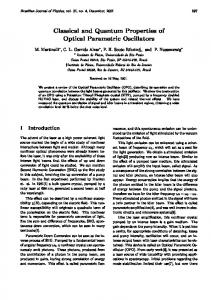
+ = 𝑡P . Inserting 𝑡2 = 𝑡P − 𝑡1 into (24), taking the derivative with respect to 𝑡1 and setting it to zero leads to a transcendental equation. It can be solved in closed form only for certain cases. Thus we resort to a numerical minimization for the remainder of this paper. The resulting process with optimized branch times is called a Maximum Availability Transition (MAT). opt opt Figure 1 shows the final energy for the system for optimized times 𝑡1 and 𝑡2 as a function of the total available process time 𝑡P . The system presented has 𝜔i = 1, 𝜔f = 0.5, and 𝐸i = 2. This leads to a FEAT time 𝜏 ≈ 0.736. From (19) follows that the minimal energy reachable is 𝐸fFEAT = 1. This can be seen in Figure 1 for times larger than the FEAT time. In the limit of the available process time towards zero the final energy approaches its limit 𝐸fSUD . This can be obtained by a sudden frequency jump 𝜔i → 𝜔f from 𝑠SUD = 𝐽(𝜔f , 𝜔i )𝑠i and leads to (1 + 𝑟2 ) 𝐸i . (26) 𝐸fSUD = 2 An interesting feature of 𝐸fmin (𝑡P ) is its graph, which seems to possess a point symmetry with respect to the point (𝜏/2, 𝐸fSUD − 𝐸fFEAT ).


6 | K. H. Hoffmann, K. Schmidt and P. Salamon, Quantum finite time availability

opt

opt

Figure 1. The final energy of a system with optimized branch times 𝑡1 and 𝑡2 as a function of the total available process time 𝑡P . The vertical red line indicates the FEAT time 𝜏 ≈ 0.736. For system details see text.

opt

opt

Figure 2. The Maximum Availability Transition (MAT) times ratio 𝑡2 /𝑡1 as a function of the available process time in units of the FEAT time 𝑡P /𝜏. Note that the MAT times ratio is always larger than the frequency ratio 𝑟. opt

opt

In Figure 2 the MAT times ratio 𝑡2 /𝑡1 is shown as a function of the available process time in units of the FEAT time 𝑡P /𝜏. The different curves represent different frequency ratios 𝑟. For process times 𝑡P approaching the FEAT time 𝜏 the MAT times ratio approaches the frequency ratio 𝑟 which it attains in the FEAT case. A surprising result is that the MAT times ratio becomes one for vanishing process times 𝑡P . This feature remains to be analyzed in the future.

6 Available work in finite time The work available in a finite process time 𝑡P depends on the frequencies 𝜔i and 𝜔f between which the process occurs and on the initial energy 𝐸i . It is determined as 𝐴(𝑡P ) = 𝐸i − 𝐸fmin (𝑡P ). The work available in a FEAT is 𝐴 FEAT = 𝐸i − 𝐸fFEAT = (1 − 𝑟)𝐸i .

(27)

The work available by a sudden frequency jump 𝜔i → 𝜔f can be determined from (26): 𝐴 SUD = 𝐸i − 𝐸fSUD =

(1 − 𝑟2 ) 𝐸i . 2

(28)

Figure 3 shows both quantities 𝐴 FEAT and 𝐴 SUD as a function of the frequency ratio 𝑟. If appropriately scaled by the initial energy of the system, 𝐴 FEAT is a linear function of 𝑟 and decays from one to zero as 𝑟 increases from zero to one. 𝐴 FEAT on the other hand decreases quadratically from 0.5 to zero.



7

Figure 3. The available work in a FEAT and the available work in a sudden frequency jump as a function of the ratio 𝑟 of the final and the initial frequency. Note that the curves approach each other for ratios close to one.

Figure 4. The quantum finite time availability in units of the FEAT availability is shown as a function of the process time in units of the FEAT time. This allows comparison of different frequency ratios 𝑟. Note that for small 𝑟 the availability stays close to one for process times down to one half of the FEAT time.

In Figure 4 the available work 𝐴(𝑡P ) is shown as a function of the available process time 𝑡P . In order to compare different 𝜔i and 𝜔f combinations we rescaled the time by the FEAT time and the available work by the FEAT availability. If the frequency ratio 𝑟 is on the order of one, then the finite time availability shows a sigmoidal behavior between 𝐴 SUD and 𝐴 FEAT which nearly looks point symmetric with respect to half the FEAT time. For smaller ratios 𝑟 this symmetry is lost and the available work decays quite slowly from its FEAT value for decreasing process time.

7 Conclusion In summary the concept of quantum finite time availability adds a new aspect to the long established finite time availability. It describes the potential work which can be obtained from a process which is too short to gain all the work from bringing a thermodynamic ensemble of quantum systems into thermal equilibrium with an environment defining the minimal value for its work parameter. The critical time in the context of parametric oscillators is the FEAT time, which is the minimal time needed to gain all potential work. One of the open questions this leaves in its wake is for which systems such FEATs exist. Can STAs followed by STIRAP-like processes [30] rearrange populations to give equilibrium states for more general systems, and thus make FEATs more generally possible? To date, the only system besides the quantum harmonic oscillator for which FEATs have been found are spin systems [31, 32].


8 | K. H. Hoffmann, K. Schmidt and P. Salamon, Quantum finite time availability Another direction of future research is the dependence of the quantum finite time availability on the limitations of the work parameter schedules. From our work on the quantum formulation of the control problem [20, 25, 29] we know that a three-jump control with two appropriately chosen wait times is optimal when the frequency ratio 𝑟 is not too large. In particular, this is the case when the ratio is obtained from the initial and final equilibrium frequencies. However, for large frequency ratios 𝑟, controls with more than three jumps may perform better [33], and thus one can introduce quantum finite time availability for different classes of FEATs depending on the number of jumps in their bang-bang controls. Regardless of how generally FEAT processes exist, our examples show the consequences of driving a system faster than the FEAT time: some of the energy must inevitably be leaked into parasitic modes. Our examples [20, 32] have a single such mode and hence are easier to analyze. Generally what we start with as availability in the system ends up either as work or as residual availability in such parasitic modes. This must perforce be the case since the processes we consider are reversible. Thus we could extract the energy from these modes by for example reversing the process we followed to reach the state, and then redoing it slowly. But this ignores the reason we sought a faster than FEAT control in the first place. Presumably this reflects an urgency that does not allow for the time required to go back and do it better. The most common reason we are aware of is if the faster than FEAT process is the adiabatic branch of a heat pump cycle and this branch is to be followed immediately by a contact to a heat bath. In such an event the temporarily foregone availability stored in the parasitic modes dissipates, even when the contact is to a heat bath at the contact temperature [34, 35]. In the latter case, the entropy increase will occur in the system via the decay of these oscillations without any change in energy. It is this feature of parasitic oscillations that points to their relevance for our discussion of availability. Availability stored in such modes is in a very precarious position – any subsequent thermal contact will decay these oscillations and dissipate the availability stored in them.

References [1] [2] [3] [4] [5] [6] [7] [8] [9] [10] [11] [12] [13] [14] [15] [16] [17]

J. W. Gibbs, A method of geometrical representations of the thermodynamic properties of substances by means of surfaces, Trans. Conn. Acad. Arts Sci. 2 (1873), 382–404. L. G. Gouy, Sur l’energie utilisable, J. Phys. 8 (1889), 501–518. A. Stodola, Steam and Gas Turbines, McGraw-Hill, New York, 1910. J. H. Keenan, Availability and irreversibility in thermodynamics, Brit. J. Appl. Phys. 2 (1951), no. 7, 183–192. J. Szargut, D. R. Morris and F. R. Steward, Exergy Analysis of Thermal, Chemical, and Metallurgical Processes, Hemisphere Publishing, New York, 1987. R. U. Ayres, L. W. Ayres and K. Martin’as, Exergy, waste accounting, and life-cycle analysis, Energy 23 (1998), no. 5, 355–363. A. Valero, Thermoeconomics as a conceptual basis for energy-ecological analysis, in: International Workshop on Advances in Energy Studies. Energy Flows in Ecology and Economy (Porto Venere 1998), 415–444. G. Tsatsaronis, Thermoeconomic analysis and optimization of energy systems, Prog. Energy Combust. Sci. 19 (1993), no. 3, 227–257. T. J. Kotas, The Exergy Method of Thermal Plant Analysis, Exergon Publishing Company, London, 2012. Y. Izumida and K. Okuda, Work output and efficiency at maximum power of linear irreversible heat engines operating with a finite-sized heat source, Phys. Rev. Lett. 112 (2014), 180603. V. Badescu, Lost available work and entropy generation: Heat versus radiation reservoirs, J. Non-Equilib. Thermodyn. 38 (2013), no. 4, 313–333. V. Madadi, T. Tavakoli and A. Rahimi, First and second thermodynamic law analyses applied to a solar dish collector, J. Non-Equilib. Thermodyn. 39 (2014), no. 4, 183–197. F. Schlögl, Produzierte Entropie als statistisches Maß, Z. Phys. 198 (1967), no. 38b, 559–568. I. Procaccia and R. D. Levine, Potential work: A statistical-mechanical approach for systems in disequilibrium, J. Chem. Phys. 65 (1976), no. 8, 3357–3364. F. Schlögl, Probability and Heat, Vieweg, Braunschweig, 1989. R. C. Tolman and P. C. Fine, On the irreversible production of entropy, Rev. Mod. Phys. 20 (1948), no. 1, 51–77. B. Andresen, M. H. Rubin and R. S. Berry, Availability for finite-time processes. General theory and a model, J. Phys. Chem. 87 (1983), no. 15, 2704–2713.



9

[18] B. Andresen, R. S. Berry, M. J. Ondrechen and P. Salamon, Thermodynamics for processes in finite-time, Accounts Chem. Res. 17 (1984), no. 8, 266–271. [19] P. Salamon and R. S. Berry, Thermodynamic length and dissipated availability, Phys. Rev. Lett. 51 (1983), no. 13, 1127–1134. [20] P. Salamon, K. H. Hoffmann, Y. Rezek and R. Kosloff, Maximum work in minimum time from a conservative quantum system, Phys. Chem. Chem. Phys. 11 (2009), 1027–1032. [21] P. Ehrenfest, Adiabatische Transformationen in der Quantentheorie und ihre Behandlung durch Niels Bohr, Naturwisschensch. 11 (1923), 543–550. [22] X. Chen, A. Ruschhaupt, S. Schmidt, A. del Campo, D. Guery-Odelin and J. Gonzalo Muga, Fast optimal frictionless atom cooling in harmonic traps: Shortcut to adiabaticity, Phys. Rev. Lett. 104 (2010), 063002. [23] X. Chen and J. Gonzalo Muga, Transient energy excitation in shortcuts to adiabaticity for the time dependent harmonic oscillator, Phys. Rev. A 82 (2010), 053403. [24] Y. Rezek, P. Salamon, K. H. Hoffmann and R. Kosloff, The quantum refrigerator: The quest for absolute zero, Europhys. Lett. 85 (2009), 30008. [25] A. M. Tsirlin, P. Salamon and K. H. Hoffmann, Change of state variables in the problems of parametric control of oscillators, Automat. Remote Control 72 (2011), no. 8, 1627–1638. [26] D. Stefanatos, J. Ruths and J.-S. Li, Frictionless atom cooling in harmonic traps: A time-optimal approach, Phys. Rev. A 82 (2010), no. 6, 063422. [27] A. del Campo, J. Goold and M. Paternostro, More bang for your buck: Super-adiabatic quantum engines, Sci. Rep. 4 (2014), 6208. [28] F. Boldt, J. D. Nulton, B. Andresen, P. Salamon and K. H. Hoffmann, Casimir companion: An invariant of motion for Hamiltonian systems, Phys. Rev. A 87 (2013), 022116. [29] P. Salamon, K. H. Hoffmann and A. Tsirlin, Optimal control in a quantum cooling problem, Appl. Math. Lett 25 (2012), 1263–1266. [30] U. Gaubatz, P. Rudecki, S. Schiemann and K. Bergmann, Population transfer between molecular vibrational levels by stimulated raman scattering with partially overlapping laser fields. A new concept and experimental results, J. Chem. Phys. 92 (1990), no. 9, 5363–5376. [31] F. Boldt, K. H. Hoffmann, P. Salamon and R. Kosloff, Time-optimal processes for interacting spin systems, Europhys. Lett. 99 (2012), 40002. [32] K. H. Hoffmann and P. Salamon, Finite-time availability in a quantum system, Europhys. Lett. 109 (2015), 40004. [33] D. Stefanatos, H. Schättler and J.-S. Li, Minimum-time frictionless atom cooling in harmonic traps, SIAM J. Control Optim. 49 (2011), 2440–2462. [34] W. Muschik, A concept of non-equilibrium temperature, Int. J. Eng. Sci. 15 (1977), no. 6, 377–389. [35] W. Muschik, Contact temperature and internal variables: A glance back, 20 years later, J. Non-Equilib. Thermodyn. 39 (2014), no. 3, 113–121. Received April 30, 2015; accepted May 5, 2015.
