Quantum phase transitions without thermodynamic limits

Quantum Phase Transitions Without Thermodynamic Limits Dorje C. Brody∗ , Daniel W. Hook∗ , and Lane P. Hughston†

arXiv:quant-ph/0511162v3 18 Apr 2006

†

∗ Blackett Laboratory, Imperial College, London SW7 2BZ, UK Department of Mathematics, King’s College London, The Strand, London WC2R 2LS, UK (Dated: February 1, 2008)

A new microcanonical equilibrium state is introduced for quantum systems with finite-dimensional state spaces. Equilibrium is characterised by a uniform distribution on a level surface of the expectation value of the Hamiltonian. The distinguishing feature of the proposed equilibrium state is that the corresponding density of states is a continuous function of the energy, and hence thermodynamic functions are well defined for finite quantum systems. The density of states, however, is not in general an analytic function. It is demonstrated that generic quantum systems therefore exhibit second-order (continuous) phase transitions at finite temperatures. PACS numbers: 05.30.-d, 05.30.Ch, 45.20.Jj

The derivation of phase transitions in quantum statistical mechanics typically requires the introduction of a thermodynamic limit, in which the number of degrees of freedom of the system approaches infinity. This limit is needed because the free energy of a finite system is analytic in the temperature. But phase transitions are associated with the breakdown of the analyticity of thermodynamic functions such as the free energy. Hence in the canonical framework the thermodynamic limit is required to generate phase transitions. Although the existence of this limit has been shown for various systems (see, e.g., [1]), the procedure can hardly be regarded as providing an adequate description of critical phenomena. One can consider, alternatively, a derivation based on the microcanonical ensemble. The usual construction of this ensemble [2] is to define the entropy by setting S = kB ln nE , where nE is the number of energy levels in a small interval [E, E + ∆E]. The temperature is then obtained from the thermodynamic relation T dS = dE. This approach, however, is not well formulated because (a) it relies on the introduction of an arbitrary energy band ∆E, and (b) the entropy is a discontinuous function of the energy. To resolve these difficulties, a scheme for taking the thermodynamic limit in the microcanonical framework was introduced in [3]. For finite systems, however, the difficulties have remained unresolved. The purpose of this paper is to demonstrate the following: (i) if the microcanonical density of states is defined in terms of the relative volume, in the space of pure quantum states, occupied by the states associated with a given energy expectation E, then the entropy of a finitedimensional quantum system is a continuous function of E, and the temperature of the system is well defined; and (ii) the density of states so obtained is in general not analytic, and thus for generic quantum systems predicts the existence of second-order phase transitions, without the consideration of thermodynamic limits. It is remarkable in this connection that similar types of second-order transitions have been observed recently for

classical spin systems, for which the associated configuration space possesses a nontrivial topological structure [4]. The paper is organised as follows. We begin with the analysis of an idealised quantum gas to motivate the introduction of a new microcanonical distribution. This leads to a natural definition of the density of states Ω(E). Unlike the number of microstates nE , the microcanonical density Ω(E) is continuous in E. As a consequence, we are able to determine the energy, temperature, and specific heat of elementary quantum systems, and work out their properties. In particular, we demonstrate that in the case of an ideal gas of quantum particles, each particle being described by a finite-dimensional state-space, the system exhibits a second-order phase transition, where the specific heat decreases abruptly. Ideal gas model. Let us consider a system that consists of a large number N of identical quantum particles (for simplicity we ignore issues associated with spinˆ total for the Hamiltonian of the statistics). We write H ˆ i (i = 1, 2, . . . , N ) for the Hamilcomposite system, and H tonians of the individual constituents of the system. The interactions between the constituents are assumed to be weak,P and hence to a good approximation we have ˆ total = N H ˆ i . We also assume that the constituents H i=1 are approximately independent and thus disentangled, so that the wave function for the composite system is approximated by a product state. If the system as a whole is in isolation, then for equilibrium we demand that the total energy of the composite system should be fixed at some value Etotal . In ˆ total i = Etotal . It follows that other words, we have hH PN ˆ h H i = E . Now consider the result of a hyi total i=1 pothetical measurement of the energy of one of the constituents. In equilibrium, owing to the effects of the weak interactions, the state of each constituent should be such that, on average, the result of an energy measurement should be the same. That is to say, in equilibrium, the state of each constituent should be such that the expectation value of the energy is the same. Therefore, writing

2 E = N −1 Etotal , we conclude that in equilibrium the gas ˆ i i = E. That is to say, the has the property that hH state of each constituent must lie on the energy surface EE in the pure-state manifold for that constituent. Since N is large, this will ensure that the uncertainty in the total energy of the composite system, as a fraction of the expectation of the total energy, is vanishingly small. Indeed, it follows from the Chebyshev inequality that " # ˆ total − Etotal | ˆ i − hH ˆ i i)2 i |H 1 h(H (1) Prob >x ≤ ˆ i i2 |Etotal | N x2 hH for any choice of x > 0. Therefore, for large N the energy uncertainty of the composite system is negligible. For convenience, we can describe the distribution of the various constituent pure states, on their respective energy surfaces, as if we were considering a probability measure on the energy surface EE of a single constituent. In reality, we have a large number of approximately independent constituents; but owing to the fact that the respective state spaces are isomorphic we can represent the behaviour of the aggregate system with the specification of a probability distribution on the energy surface of a single “representative” constituent. Microcanonical equilibrium. In equilibrium, the distribution is uniform on the energy surface, since the equilibrium distribution should maximise an appropriate entropy functional on the set of possible probability distributions on EE . From a physical point of view we can argue that the constituents of the gas approach an equilibrium as follows: On the one hand, weak exchanges of energy result in all the states settling on or close to the energy surface; on the other hand, the interactions will induce an effectively random perturbation in the Schr¨odinger dynamics of each constituent, causing it to undergo a Brownian motion on EE that in the long run induces uniformity in the distribution on EE . We conclude that the equilibrium configuration of a quantum gas is represented by a uniform measure on an energy surface of a representative constituent of the gas. The theory of the quantum microcanonical equilibrium state presented here is analogous in many respects to the symplectic formulation of the classical microcanonical ensemble described in [5]. There is, however, a subtle difference. Classically, the uncertainty in the energy is fully characterised by the statistical distribution over the phase space, and for a microcanonical distribution with support on a level surface of the Hamiltonian the energy uncertainty vanishes. Quantum mechanically, however, although the statistical contribution to the energy variance vanishes, there remains an additional purely quantum-mechanical contribution. Hence, although the energy uncertainty for the composite system is negligible for large N , the energy uncertainties of the constituents will not in general vanish. An expression for ∆H will be given in equation (9) below.

Density of states. To describe the equilibrium represented by a uniform distribution on the energy surface EE , it is convenient to use the symplectic formulation of quantum mechanics. Let H denote the Hilbert space of states associated with a constituent. We assume that the dimension of H is n + 1. The space of rays through the origin of H is a manifold Γ equipped with a metric and a symplectic structure. The expectation of the Hamiltonian along a given ray of H then defines a Hamiltonian ˆ i |ψi/hψ|ψi on Γ, where the ray function H(ψ) = hψ|H ψ ∈ Γ corresponds to the equivalence class |ψi ∼ λ|ψi, λ ∈ C\0. The Schr¨odinger evolution on H is a symplectic flow on Γ, and hence we may regard Γ as the quantum phase space. Our approach to quantum statistical mechanics thus unifies two independent lines of enquiry, each of which has attracted attention in recent years: the first of these is the “geometric” or “dynamical systems” approach to quantum mechanics, which takes the symplectic structure of the space of pure states as its starting point [6]; and the second of these is the probabilistic approach to the foundations of quantum statistical mechanics in which the space of probability distributions on the space of pure states plays a primary role [7]. The level surface EE in Γ is defined by H(ψ) = E. The entropy associated with the corresponding microcanonical distribution is S(E) = kB ln Ω(E), where Z δ(H(ψ) − E)dVΓ . (2) Ω(E) = Γ

Here dVΓ denotes the volume element on Γ. In a microcanonical equilibrium the temperature is determined intrinsically by the thermodynamic relation T dS = dE, which implies that kB T = Ω(E)/Ω′ (E), where Ω′ (E) = dΩ(E)/dE. Since the density of states Ω(E) is differentiable, the temperature is well-defined. Other thermodynamic quantities can likewise be precisely determined. For example, the specific heat C(T ) = dE/dT is given by C = kB (Ω′ )2 /[(Ω′ )2 − ΩΩ′′ ]. Consider a large system composed of two independent parts, each in a state of equilibrium. Each subsystem is thus described by a microcanonical state with support on the Segr´e variety corresponding to disentangled subsystem states. Let us write Ω1 (E1 ) and Ω2 (E2 ) for the associated state densities, where E1 and E2 are the initial energies of the two systems. Now imagine that the two systems interact weakly for a period of time, during which energy is exchanged, following which the systems become independent again, each in a state of equilibrium. As a consequence of the interaction the state densities of the systems will now be given by expressions of the form Ω1 (E1 + ǫ) and Ω2 (E2 − ǫ), for some value of the exchanged energy ǫ. The value of ǫ can be determined by the requirement that the total entropy S(E) = kB ln[Ω1 (E1 +ǫ)Ω2 (E2 −ǫ)] should be maximised. A short calculation shows that this condition is satisfied if and only if ǫ is such that the temperatures of the two

3 systems are equal. This argument shows that the definition of temperature that we have chosen is a natural one, and is physically consistent with the principles of equilibrium thermodynamics. Phase transitions. The quantum microcanonical ensemble introduced here is applicable to any isolated finite-dimensional quantum system for which the ideal gas approximation is valid. The volume integral in (2) can be calculated by lifting the integration from Γ to H and imposing the constraint that the norm of |ψi is unity. Then we can write: Z   hψ|H|ψi ˆ 1 − E dVH , (3) δ(hψ|ψi − 1) δ Ω(E) = π H hψ|ψi where dVH is the volume element of H. Making use of the standard Fourier integral representation for the delta function, and diagonalising the Hamiltonian, we find that (3) reduces to a series of Gaussian integrals (see [8] for details). Performing the ψ-integration we then obtain the following integral representation for the density of states: Ω(E) = (−iπ)n

Z∞

−∞

dν 2π

Z∞

−∞

n+1 dλ i(λ+νE) Y 1 e . (4) 2πi (λ + νEl )

 δj −1 m 1 d (−1)m−1 π n Y Ω(E) = (n − 1)! j=1 (δj − 1)! dEj m X

(Ek − E)n−1

k=1

m Y 1{Ek >E}

l6=k

El − Ek

,

(5)

where 1{A} denotes the indicator function (1{A} = 1 if A is true, and 0 otherwise). In (5) we let m denote the number of distinct eigenvalues Ej (j = 1, 2, . . . , m), and we let δj denoteP the multiplicity associated with the energy Ej . Thus m j=1 δj = n + 1. In the nondegenerate case, for which δj = 1 for j = 1, 2, . . . , m, we have n+1 n+1 Y 1{Ek >E} (−π)n X n−1 Ω(E) = . (Ek − E) (n − 1)! El − Ek k=1

(6)

l6=k

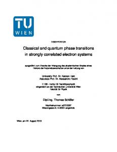
With these expressions at hand we proceed now to examine some explicit examples. Nondegenerate spectra. In the case of a Hamiltonian with a nondegenerate spectrum of the form Ek = ε(k − 1), k = 1, 2, . . . , n + 1, where ε is a fixed unit of energy, the density of states (6) reduces to Ω(E) = ε−1

n n−1 (−π)n X (−1)k (k − E/ε) . (n − 1)! k!(n − k)! k>E/ε

WHEL

3

2

1

E 1

2

3

4

5

FIG. 1: Density of states Ω(E) for nondegenerate (n + 1)level systems for n = 3, 4, 5, with energy eigenvalues Ek = k (k = 0, . . . , n). Ω(E) is n − 2 times differentiable in E.

l=1

The two integrals appearing here correspond to the deltafunctions associated with the energy constraint H(ψ) = E and the norm constraint hψ|ψi = 1. Carrying out the integration we find that the density of states is given by

×

We see that Ω(E) is a polynomial of degree n − 1 in each interval E ∈ [Ej , Ej+1 ], and that for all values of E it is at least n − 2 times differentiable. In Fig. 1 we plot Ω(E) for several values of n. For a system in equilibrium the accessible values of E are those for which Ω′ (E) ≥ 0. States for which Ω′ (E) < 0 have “negative temperature” in the sense of Ramsey [9].

(7)

The structure of the space of pure states in quantum mechanics is intricate, even for relatively elementary systems. In particular, as the value of the energy changes, the topological structure of the energy surface undergoes a transition at each eigenvalue [10]. For example, in the case of a nondegenerate three-level system, the topology of the energy surface changes according to: Point → S 3 → S 1 × R2# → S 3 → Point, as the energy is raised from Emin to Emax (R2# denotes a two-plane compactified into S 2 at a point corresponding to the intermediate eigenstate). These structural changes in the energy surfaces induce a corresponding nontrivial behaviour in the thermodynamic functions. As an illustration we consider a four-level system and compute the specific heat as a function of temperature. The result is shown in Fig. 2, where we observe that the specific heat drops abruptly from 2kB to 21 kB at the critical temperature Tc defined by kB Tc = 21 ε. Therefore, this system exhibits a second-order phase transition, in this case at the critical energy Ec = ε. This example shows that the relationships between phase transitions and topology discovered recently in classical statistical mechanics [11] carry over to the quantum domain where, arguably, they may play an even more basic role. For a system with a larger number of nondegenerate eigenstates, the specific heat also increases abruptly as T is reduced. In this case the specific heat is continuous, and the discontinuity is in a higher-order derivative of the energy. For a system with n + 1 nondegenerate energy eigenvalues, the (n − 1)-th derivative of the energy with respect to the temperature has a discontinuity. The phe-

4 nomenon of a continuous phase transition is generic, and is also observed if the eigenvalue spacing is not uniform. Degenerate spectra. In a system with a degenerate spectrum, the phase transition can be enhanced. In particular, the volume of EE increases more rapidly as E approaches the first energy level from below, if this level is degenerate. This leads to a more abrupt drop in the specific heat (Fig. 2). CHTL 3 2.5 2 1.5 1

at E = Emax we note that the first moment of Ω(E) is given by the integral of H(x) over Γ. Hence by use of a trace identity obtained in [12] we have Z Z Emax πn ¯ H(ψ) dVΓ = u Ω(u) du = H. (10) n! Γ Emin However, the integral of Ω(E) is the volume π n /n! of Γ, and the desired result follows. Using the explicit formulae obtained earlier for Ω(E) we are then able to calculate the energy uncertainty associated with the equilibrium state of a finite quantum system. It remains to be seen whether the new ensemble can be put to the test in some definitive way, and in particular whether the phase transitions it predicts actually correspond to observable phenomena. DCB acknowledges support from The Royal Society. The authors thank M. Kastner, T.W.B. Kibble, and an anonymous referee for helpful comments.

0.5 T 0.25

0.5

0.75

1

1.25

1.5

FIG. 2: Specific heat for a nondegenerate four-level system (dotted line, n = 3, Ej = 0, 1, 2, 3), a four-level system having a degenerate first excited state (dashed line, n = 4, Ej = 0, 1, 1, 2, 3), and a quantum Ising chain (solid line, J = 1/4, B = 1). In the quantum Ising chain, we have C(T ) ∼ (T − Tc )−2 away from Tc , whereas in the vicinity of Tc we have C(T ) ∼ (T − Tc )−13 for T > Tc . (We set kB = 1 here.)

As an example, we consider a quantum Lenz-Ising ferromagnetic P chain with threePspins. The Hamiltonian is ˆ = −J 3 σzk σzk+1 − B 3 σzk , where σzk denotes H k=1 k=1 the third Pauli matrix for spin k, and J, B are constants. We have in mind a gas of weakly interacting molecules, each modelled by a strongly-interacting quantum Ising chain. The eigenvalues of the Hamiltonian are E1 = −3J − 3B, E2,3,4 = J − B, E5,6,7 = J + B, and E8 = −3J + 3B. As the temperature is reduced, the specific heat grows rapidly in the vicinity of the critical point Tc = (2J + B)/3kB (Fig. 2), where the system exhibits a discontinuity in the second derivative of the specific heat. We note that when B is small the critical temperature is close to that of the classical mean-field Ising model. Density matrix and energy uncertainty. Finally, we show the existence of a natural energy band associated with the quantum microcanonical distribution. The microcanonical density matrix for the energy E is Z 1 ˆ µ ˆE = δ(H(ψ) − E)Π(ψ) dVΓ . (8) Ω(E) Γ

ˆ Here Π(ψ) = |ψihψ|/hψ|ψi denotes the projection operator onto the state |ψi ∈ H corresponding to the point ψ ∈ Γ. The squared energy uncertainty is (∆H)2 = ˆ 2 . A calculation then shows that ˆ 2 ) − [tr(ˆ µE H)] tr(ˆ µE H Z n+1 E ¯ 2 (H − u) Ω(u) du, (9) (∆H) = Ω(E) Emin ¯ = tr(H)/(n ˆ where H + 1) denotes the uniform average of the energy eigenvalues. To check that ∆H vanishes

[1] D. Ruelle, Statistical mechanics: rigorous results (Imperial College Press, London, 1999). [2] K. Huang, Statistical mechanics, 2nd ed. (John Wiley and Sons, New York, 1987). [3] R.B. Griffiths, J. Math. Phys. 6 1447 (1965). [4] M. Kastner and O. Schnetz, J. Stat. Phys. 122 1195 (2006). [5] A.I. Khinchin, Mathematical foundations of statistical mechanics (Dover, New York, 1949); C. J. Thompson, Mathematical statistical mechanics (Macmillan, New York, 1972). [6] T.W.B. Kibble, Commun. Math. Phys. 65, 189 (1979); J. Anandan and Y. Aharonov, Phys. Rev. Lett. 65, 1697 (1990); A. Ashtekar and T.A. Schilling, in On Einstein’s Path, A. Harvey, ed. (Springer-Verlag, Berlin, 1998); A. Benvegn` u, N. Sansonetto, and M. Spera, J. Geom. Phys. 51, 229 (2004). [7] E.T. Jaynes, Phys. Rev. 108, 171 (1957); A.Y. Khinchin, Mathematical foundations of quantum statistics (Graylock Press, Toronto, 1960); D.C. Brody and L.P. Hughston, J. Math. Phys. 39, 6502 (1998); S. Goldstein, J.L. Lebowitz, R. Tumulka, and N. Zangh`ı, Phys. Rev. Lett. 96, 050403 (2006); G. Jona-Lasinio and C. Presilla, quant-ph/0603245. [8] D.C. Brody, D.W. Hook, and L.P. Hughston, quant-ph/0506163; C.M. Bender, D.C. Brody, and D.W. Hook, J. Phys A38, L607 (2005). [9] N.F. Ramsey, Phys. Rev 103, 20 (1956). [10] D.C. Brody and L.P. Hughston, J. Geom. Phys. 38, 19 (2001). [11] R. Franzosi and M. Pettini, Phys. Rev. Lett. 92, 060601 (2004); M. Kastner, ibid. 93, 150601 (2004); M. Kastner, Physica A359, 447 (2006). [12] G.W. Gibbons, J. Geom. Phys. 8, 147 (1992).