Quantum Probability and Quantum Information Theory Hans Maassen Radboud University, Toernooiveld 1, 6525 ED Nijmegen, Netherlands,
[email protected]
1 Introduction From its very birth in the 1920’s, quantum theory has been characterized by a certain strangeness: its seems to run counter to the intuitions that we humans have about the world we live in. According to these ‘realistic’ intuitions all things have their definite place and sharply determined qualities, such as speed, color, and weight. Quantum theory, however, refuses to precisely pinpoint them. With respect to this apparent shortcoming of the theory different points of view can be taken. It could be suspected that quantum theory is incomplete, that it gives a coarse description of a reality that is actually more refined. This is the viewpoint once taken by Einstein, and it still has adherents today. It calls for a search for finer mathematical models of physical reality, often referred to as ‘hidden variable models’. One such attempt is Bohm’s theory of non-relativistic quantum mechanics. However, the work of John Bell in the 60’s and of Alain Aspect in the 80’s strongly favors the opposite point of view: their work has made clear that such models with an underlying realistic structure are necessarily afflicted with a certain weakness: they must at least allow action at a distance. This we regard as a bad property for a theory which aims to describe a physical world where no signals have been observed to travel faster than light. And apart from that, the hidden variable theories which have been found so far are highly artificial and do not predict any new phenomena. It is for these reasons that we decide to accept quantum theory with its inherent strangeness. We note, in passing, that that there is no paradox in quantum mechanics: the theory does not contradict itself. It is only at variance with our intuition, which we think must be adapted.
2
Hans Maassen
1.1 Quantum Probability So quantum mechanics does not predict the results of physical experiments with certainty, but calculates probabilities for their possible outcomes. Now, the mathematical theory of probability obtained a unified formulation in the 1930’s, when Kolmogorov introduced his axioms, defining the universal structure (Ω, Σ,P) I of a probability space. For a long time this theory of probability (dealing with probability distributions, stochastic processes, Markov chains, martingales, etc.) remained completely separate from the mathematical development of quantum mechanics (involving vectors in a Hilbert space, hermitian operators, unitary transformations, and such like). In the 1970’s and 1980’s people around Accardi, Lewis, Davies, K¨ ummerer, building on ideas of von Neumann’s and Segal’s, developed a unified framework, a generalized, ‘non-commutative’, probability theory, in which classical probability theory and quantum mechanics can be discussed in unison. It consists of ordinary Hilbert space quantum theory, with the emphasis moved towards operators on Hilbert space, and the algebras which they generate. The main objective of this course is to sketch the outlines of this framework, and show its usefulness for information theory. 1.2 Quantum Information In Shannon’s (classical) information theory, a single unit, the bit, serves to quantify all forms of information, be it in print, in computer memory, CDROM or strings of DNA. Such a single unit suffices, because different forms of information can be converted into each other by copying, according to fixed ‘exchange rates’. The physical states of quantum systems, however, cannot be copied into such ‘classical’ information, but can be converted into each other. This leads to a new unit of information: the qubit. Quantum Information theory studies the handling of this new form of information by information-carrying channels. We shall treat the basic properties of these channels, and some impossibilities as well as new possibilities connected with quantum information. 1.3 Quantum Computing It was Richard Feynman who first thought of actually employing the strangeness of quantum mechanics to do things that would be impossible in a classical world. The idea was developed in the 1980’s and 1990’s by David Deutsch, Peter Shor, and many others into a flourishing branch of science called ‘quantum computing’: how to make quantummechanical systems perform calculations more efficiently than ordinary computers can do. This research is still in a predominantly theoretical stage: the quantum computers actually built are as yet extremely primitive and can by no means compete with even the simplest pocket calculator, but expectations are high.
Quantum Probability
3
1.4 This Course We start with an introduction to quantum probability. In Section 2 we demonstrate the ‘strangeness’ of quantum phenomena by very simple polarization experiments, culminating in Bell’s famous inequality, tested in Aspect’s equally famous experiment. Bell’s inequality is a statement in classical probability that is violated in quantum probability and in reality. Taking polarizers as our starting point, in Sections 3 and 4 we build up the new probability theory in terms of algebras of operators on a Hilbert space. In Section 5 operations on these algebras will be characterized, and some aspects in which they differ from classical physical operations They are subject to certain strange limitations: the impossibility of copying, of coding information into bits, of jointly measuring incompatible observables, of observation without perturbing the object (Cf. Section 6.) But they also open up surprising possibilities: entangling remote systems, teleportation of this entanglement, sending two bits in a single qubit. (Cf. Section 7.) We shall leave the further luring perspectives to other courses in this School: highly efficient algorithms for sorting, Fourier transformation and factoring very large numbers.
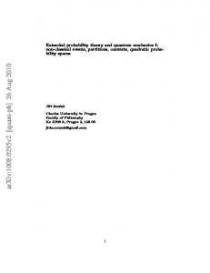
2 Why Classical Probability does not Suffice (This section is based on [6].) 2.1 An Experiment with Polarizers To start with, we consider a simple experiment. In a beam of light of a fixed color we put a pair of polarizing filters, each of which can be rotated around the axis formed by the beam. As is well known, the light falling through both filters changes in intensity when the filters are rotated relative to each other. Starting from the orientation where the resulting intensity is maximal, and rotating one of the filters through an angle α, the light intensity decreases with α, vanishing for α = 12 π. If we call the intensity of the beam before the filters I0 , after the first I1 , and after the second I2 , then I1 = 12 I0 , (we assume the original beam to be unpolarized), and I2 = I1 cos2 α.
(1)
So far the phenomenon is described well by classical physics. During the last century, however, it has been observed that for very low intensities (monochromatic) light comes in small packages, which were called photons, whose energy depends on the color, but not on the total intensity. So the intensity must be proportional to the number of these photons, and formula (1) must be given a statistical meaning: a photon passing through the
4
Hans Maassen
I0
I1
I2
α
Fig. 1. Two polarizers in conjunction
first filter has a probability cos2 α to pass through the second. Formula (1) then only holds on the average, for large numbers of photons. Thinking along the lines of classical probability, we may associate to a polarization filter in the direction α a random variable Pα , taking the value Pα (ω) = 0 if the photon ω is absorbed by the filter and Pα (ω) = 1 if it passes through. For two filters in the directions α and β these random variables then should be correlated as follows: E(P I α Pβ ) = P[P I α = 1 and Pβ = 1] =
1 2
cos2 (α − β).
(2)
Here we hit on a difficulty: the function on the right hand side is not a possible correlation function! This can be seen as follows. Take three polarizing filters, having polarization directions α1 , α2 and α3 respectively. We put them on the optical bench in pairs. They should give rise to random variables P1 , P2 and P3 satisfying E(P I i Pj ) = 12 cos2 (αi − αj ). Proposition 1. (Bell’s 3 variable inequality) For any three 0-1-valued random variables P1 , P2 , and P3 on a probability space (Ω,P) I the following inequality holds: I 1 = 1, P2 = 0] + P[P I 2 = 1, P3 = 0]. P[P I 1 = 1, P3 = 0] ≤ P[P Proof. P[P I 1 = 1, P3 = 0] = P[P I 1 = 1, P2 = 0, P3 = 0] + P[P I 1 = 1, P2 = 1, P3 = 0] ≤ P[P I 1 = 1, P2 = 0] + P[P I 2 = 1, P3 = 0]. t u In our example, we have P[P I i = 1, Pj = 0] = P[P I i = 1] − P[P I i = 1, Pj = 1] = 21 − 12 cos2 (αi − αj ) = 12 sin2 (αi − αj ). Bell’s inequality thus reads
Quantum Probability 1 2
sin2 (α1 − α3 ) ≤
1 2
sin2 (α1 − α2 ) +
1 2
5
sin2 (α2 − α3 ),
which is clearly violated for the choices α1 = 0, α2 = 16 π and α3 = 31 π, where it says that 1 1 3 ≤ + . 8 8 8 This example suggests that classical probability cannot even describe this simple experiment! Remark The above calculation could be summarized as follows: we are in fact looking for a family of 0-1-valued random variables (Pα )0≤α