Density functional theory can accurately predict chemical and mechanical properties of nano- structures, although at a high computational cost.
Copyright © 2007 American Scientific Publishers All rights reserved Printed in the United States of America
Journal of Nanoscience and Nanotechnology Vol. 8, 1–12, 2007
Quasicontinuum-Like Reduction of Density Functional Theory Calculations of Nanostructures Dan Negrut1� ∗ , Mihai Anitescu2 , Anter El-Azab3 , and Peter Zapol4 1
Materials Science Program, Department of Mechanical Engineering, The University of Wisconsin, Madison, WI 53706, USA 2 Mathematics and Computer Science Division, Argonne National Laboratory, Argonne, IL 60439, USA 3 School of Computational Science, Florida State University, Tallahassee, FL 32306, USA 4 Materials Science and Chemistry Divisions, Argonne National Laboratory, Argonne, IL 60439, USA Density functional theory can accurately predict chemical and mechanical properties of nanostructures, although at a high computational cost. A quasicontinuum-like framework is proposed to substantially increase the size of the nanostructures accessible by simulations. It takes advantage of the near periodicity of the atomic positions in some regions of nanocrystalline materials to establish an interpolation scheme for the electronic density in the system. The electronic problem embeds interpolation and coupled cross-domain optimization techniques through a process called electronic reconstruction. For the optimization of nuclei positions, computational gains result from explicit consideration of a reduced number of representative nuclei interpolating the positions of the rest of nuclei following the quasicontinuum paradigm. Numerical tests using the Thomas-FermiDirac functional demonstrate the validity of the proposed framework within the orbital-free density functional theory.
Keywords:
Nanostructures have dimensions in the range of 1∼100 nm and typically contain 102 ∼108 atoms. Density functional theory (DFT) methods within the Kohn-Sham approach1 are typically applied to systems with fewer than 100 atoms. Contemporary implementations of order-N methods2 such as SIESTA,3 ONETEP,4 and CONQUEST5 that exhibit linear scaling of computation time with system size enable an increase in the number of atoms by one to two orders of magnitude. Studies of larger systems such as quantum dots and nanoparticles at the electronic structure level resort to tight-binding methods,6 kp method,7 or empirical pseudopotential method.8 These methods require parameterizations to empirical or first-principles data, and do not typically reproduce all structural and electronic properties with high accuracy across a full range of possible geometries. Even larger system sizes are accessible to interatomic potential methods but these methods cannot account for spin and charge relaxation and conjugation effects, which are important in modeling reactions, electronic excitation, and bond breaking processes. Therefore, new computational paradigms are needed that enable larger scale electronic structure calculations. ∗
Author to whom correspondence should be addressed.
J. Nanosci. Nanotechnol. 2007, Vol. 8, No. 4
A combination of methods with different fidelity is often used to reduce computational effort if only local information is needed with high accuracy. An example of such an approach is the ONIOM method9 for computations of chemical properties. However, such schemes have an inherent problem with conditions at the boundaries of different fidelity regions. Another approach to reduce computational effort, called the quasicontinuum method, is based on explicit treatment of only representative atoms and on interpolations for the rest. It has been successfully used in atomistic studies of mechanical properties with classical potentials and recently with electronic-level calculations. This type of approach is particularly suitable for many nanostructures because large regions of the structures are perturbed relatively little as compared to periodic structures and, therefore, can be treated by using interpolation schemes. The present work proposes a quasicontinuum-like technique that renders electronic structure information at the nanoscale. The proposed methodology follows in the steps of the quasicontinuum approach10–12 for mechanical analysis at the nanoscale. Specifically, this is an extension of the work in,11� 12 because, rather than considering a potentialbased interatomic interaction that has a limited range of validity and is difficult to generalize to inhomogeneous
1533-4880/2007/8/001/012
doi:10.1166/jnn.2007.013
1
RESEARCH ARTICLE
1. INTRODUCTION
RESEARCH ARTICLE
Quasicontinuum-Like Reduction of DFT Calculations of Nanostructures
materials, the methodology proposed uses an ab initio method. At the same time it is a generalization of the method proposed in Ref. [10] because, rather than considering electron density within each mesh discretization element separately, the proposed method treats the electronic density distribution in all elements in an overall optimization framework. The approach proposed does not rely on a strict periodicity assumption; it merely assumes that the material displays a nearly periodic structure in certain regions of the nanostructure. However, in order to bridge the gap between subatomic scale associated with the electron density and the nanoscale associated with the structures investigated, we have assumed that almost everywhere in the nanostructure the optimized structure results in only small deformations of periodic structure. This assumption is referred to as near-periodicity, because the nonperiodic part of the state variables is approximated as a macroscopic smoothly varying field. As explained later, the nearperiodicity assumption enables the use of interpolation for electronic structure reconstruction. A second assumption made is that only small deformations are present in most of the material. The nanostructure is considered to have an initial reference configuration D0 ⊂ �3 . The structure undergoes a deformation described by a deformation mapping ��r0 � t� ∈ �3 , which gives the location r in the global Cartesian reference frame of each point r0 represented in the undeformed material frame. As indicated, the mapping might depend on time t. The variable t does not necessarily represent the time contemporary with the structure under consideration. In a static simulation framework this variable might be an iteration index of an optimization algorithm that solves for the system ground state. The components of the deformation gradient F are introduced as
� FiJ = 0i
rJ where upper-case indices refer to the material frame, and lower-case indices to the Cartesian global frame. Thus, F = 0 �, where 0 represents the material gradient operator. Using the repeated index summation rule, the deformation of an infinitesimal material neighborhood dr0 about a point r0 of D0 is expressed as dri =
FiJ drJ0
If u = r − r0 , the concept of small distortion is equivalent to requiring that the spectral radius of the 3 × 3 matrix � = u�r0 � be sufficiently small; that is, F �� 0 u�r0 �� < � is expected to hold almost everywhere in the domain D0 , for a suitable chosen value of �. With the two assumptions introduced, computational savings are due to a two-tier interpolation-based approach 2
Negrut et al.
that reduces the dimension of the problem. First, the electronic structure will be evaluated in some domains by interpolation using adjacent regions in which a DFTbased approach is used to accurately solve the electronic structure problem; this procedure is called electronic density reconstruction. Second, the positions of the nanostructure nuclei will be expressed in terms of the positions of a reduced set of so-called representative nuclei, repnuclei. The proposed approach solves only for the positions of these repnuclei; the entire deformation field (mapping) is defined based on an appropriate representation for ��r0 � t�. Following the quasicontinuum paradigm,11� 12 we define this mapping based on the displacement of repnuclei: � ��r0 � t� = ��r0 RJ0 ���RJ0 � t� (1) J ∈�
where � represents the index set associated with the repnuclei. Once the displacements of the repnuclei ��RJ0 � t� for J ∈ � are available, the displacement of any point in the nanostructure is obtained by interpolation using the shape functions �.
2. THE IONIC PROBLEM AND QUASICONTINUUM APPROACH Finding the stable configuration of a nanostructure (called hereafter the Ionic Problem) reduces to minimizing the total energy Etot with respect to the positions of the nuclei. More precisely, the equilibrium configuration of a nanostructure is provided by that distribution of the nuclei that minimizes the energy Etot = Ee + Eext + Enn where Enn is the internuclear interaction energy, Ee is the electronic ground-state energy for the corresponding nuclear distribution, and Eext is the electron-nuclei interaction energy defined as � Eext ���r�� ˆ �RI �� = − ��r�V ˆ ext �r� �RI ��dr =−
M � � A=1
ˆ ZA ��r� dr r − RA
ˆ ZA ��r� dr is the ionic r − RA potential, which depends on the positions of the nuclei �RI �, and ZA is the atomic number of nucleus A. The electronic structure computation is approached here as the solution of a constrained minimization problem according to the� Hohenberg-Kohn theorem,13 min� Etot ���r��, subject to ��r�dr = Ne , where Ne represents the number of electrons present in the system. The solution to this problem depends parametrically on the locations of the nuclei RI , I = 1� � � � � M, a consequence of where Vext �r� �RI �� =
�M
A=1
J. Nanosci. Nanotechnol. 8, 1–12, 2007
Negrut et al.
Quasicontinuum-Like Reduction of DFT Calculations of Nanostructures
the Born-Oppenheimer approximation. Subsequently, the optimization of nuclei positions in the entire system is the solution of min�RI � Etot . Let us consider the optimization problem min Etot = min Ee + Eext + Enn �RI �
�RI �
subject to the constraint that for a nuclear configuration �RI � the energy Ee is the electron ground-state energy. Under this assumption, the first-order optimality conditions from the Hellmann-Feynman theorem14 yield FK =
Eext Enn + =0
RK
RK
where FK , K = 1� � � � � M, is interpreted as the force acting on nucleus K and Enn =
M �
M �
ZA ZB A=1 B=A+1 R B − RA
The Hellmann-Feynman theorem leads, for each nucleus K, to �
��r� ˆ
J. Nanosci. Nanotechnol. 8, 1–12, 2007
(3) This effectively reduces the dimension of the problem from 3M (the �x� y� z� coordinates of the nuclei), to 3Mrep , where Mrep is the number of nodes in the atomic mesh, which is the number of elements in �. Following the quasicontinuum paradigm, the selection and the number of the repnuclei is based on an energetic argument and tailors the computational mesh to the structure of the deformation field.11 The sum in the expression of FJ above is most likely not going to be the simulation bottleneck (solving the electron problem for �ˆ is significantly more demanding), but fast-multipole methods17–19 can be considered to speed the summation. Denoting by Pi , i = 1� � � � � Mrep , the position of the representative nucleus ni , we can group the set of nonlinear equations of Eq. (3) into a nonlinear system that is solved for the relaxed configuration of the structure: f1 �P1 � P2 � � � � � PMrep � = 0 f2 �P1 � P2 � � � � � PMrep � = 0 ··· fMrep �P1 � P2 � � � � � PMrep � = 0 where fJ is obtained based on Eq. (3). The solution of this system is found by a Newton-like method. Evaluating the Jacobian information is straightforward and not detailed here. We note that in Eq. (3) a connection is made back to Eq. (1); the position of an arbitrary nucleus A in cell ! is computed based on interpolation using the nodes � �!�, one of many choices available (one could consider repnuclei from neighboring cells, for instance). Effectively, this provides in Eq. (1) an expression for ��RA0 � t�, which depends only on J ∈ � �!� rather than J ∈ �.
3. THE ELECTRONIC PROBLEM The electronic problem refers to the computation of the ground-state electron density given the positions of nuclei in the nanostructure. Scaling considerations and accuracy requirements established DFT as the most viable candidate 3
RESEARCH ARTICLE
M � RA − R K r − RK dr + ZA =0 3 r − RK 3 R A − RK A=1� A =K (2) which thus allows one to solve the nuclear equilibrium problem by using only the ground state solutions of the electron density problem to find forces on ions to the first order and not the values and the derivatives of the kinetic and exchange energies. Once the electron density is available, the equilibrium conditions FK = 0, K = 1� � � � � M, can be imposed right away. The major computational consequence of this result is that how the actual ground state electron density ��r� ˆ was obtained is irrelevant; there is also no need to have an explicit energy functional of the electron density �. Moreover, the gradient of the energy with respect to the atomic positions at the current electron density has the same property.15 Therefore, the groundstate electron density can be computed with a stand-alone software package that requires only the current atomic positions. Since we use an iterative technique to solve the electronic density problem this means that we compute only an approximation of the ground state energy �. ˆ Therefore, the expression of FK , K = 1� 2� � � � � M in (2) is only an approximation of the gradient of the energy with respect to �RK �, K = 1� 2� � � � � M. Nonetheless, for optimization algorithms of the type discussed here, FK , K = 1� 2� � � � � M need not be calculated exactly, rather they should only provide a search vector whose angle with the exact gradient is bounded away from �/2.16 Therefore, the approach proposed can tolerate inexact values of the ground density �. ˆ When a local quasicontinuum approach is used, the equilibrium conditions are imposed only for repnuclei, that is, only for J ∈ �. The positions of the remaining atoms
FK =
in the system is then expressed in terms of the positions of the repnuclei. The repnuclei become the nodes of an atomic mesh, and interpolation is used to recover the position of the remaining nuclei. Concretely, if the atomic mesh is denoted by �, ! is an arbitrary cell in this mesh, � �!� represents the set of nodes associated with cell !, and �L is the shape function associated with node L in cell !, � r −RJ ˆ dr FJ = ��r� r −RJ 3 � 0 �� L∈� �!� RL �L �RA �−RJ + ZA � = 0� J ∈ � L∈� �!� RL �L �RA0 �−RJ 3 !∈� A∈!
Quasicontinuum-Like Reduction of DFT Calculations of Nanostructures
for handling this task. In a general form, the electronic contributions to the total energy in a density functional framework can be written as
RESEARCH ARTICLE
Ee ��� = T ���r�� + E
Har
which has been further improved on31–33� 20 � THyb ��� = TvW ��� + *) T)
xc
���r�� + E ���r��
where T ���r�� is the kinetic energy functional, E Har ���r�� is the electron–electron Coulomb repulsion energy, and E xc ���r�� is the exchange and correlation energy. The ground-state electron density is the function ��r� ˆ that minimizes Ee ��� + Eext ���r�� �RI �� with respect to the electron density subject to a charge conservation constraint, � ��r�dr ˆ − N = 0, and the requirement that the density stay nonnegative. The orbital-free DFT (OFDFT) methods (see, for instance, Ref. [20]), based on the explicit approximations to the unknown exact functional are attractive as they are numerically easier to formulate and solve than the most widely used Kohn-Sham approach (KS-DFT)1 and there is no need for orbital localization and orthonormalization. Compared to the KS-DFT approaches that typically require the solution of a nonlinear algebraic eigenvalue problem, the OFDFT approaches result in optimization problems based on a methodology that scales linearly and is relatively simple to implement. The main difficulty lies in providing good quality approximate functionals, since the exact functionals are not known. This is particularly true in the case of the kinetic energy functional, which is otherwise easily obtained in traditional KS-DFT. Efforts to find accurate functionals have been quite successful for several simple metal systems. OFDFT has recently been used in molecular dynamics simulations for accurate representation of interatomic forces in order to reproduce and provide an explanation for calorimetry results in Na clusters,21 for the studies of several thousand atoms near a metallic grain boundary,22 for predicting of the dislocation nucleation during nanoindentation of Al3 Mg (Ref. [23]) used in combination with the quasicontinuum method,12� 24 and for the metal-insulator transition in a two-dimensional array of metal nanocrystal quantum dots.25 Approximations for the exchange and correlation energy functionals, K���, are discussed, for instance, in Refs. [26] and [27]. Providing suitable expressions for the kinetic energy functional remains a challenging task and, because of reduced transferability, is the factor that prevents widespread use of the approach. The simplest explicit functional is due to Thomas and Fermi28� 29 � 5 TTF ��� = CF � 3 �r�dr where CF is a constant. This crude approximation has been improved upon by the von Weizsäcker form of the kinetic energy functional,30 1 � ��r� 2 TvW ��� = TTF ��� + dr 8 ��r� 4
Negrut et al.
T) =
� �
)
�) �r��) �r� �w) �r − r� � ��r��drdr�
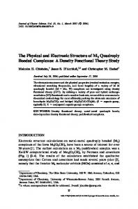
where the function w) �r − r� � ��r�� is an electron densitydependent kernel that is formulation dependent. Within the framework of OFDFT for electronic structure computation a model reduction approach is pursued that relies on the near-periodicity assumption introduced above.34� 35 The entire domain of interest is first meshed and divided into subdomains. Using a finite element approach one can express the kinetic, exchange correlation, Coulomb, and electron-nuclei interaction energies in terms of the values of the electron density at grid points. Since the bulk of a nanostructure often displays quasiperiodic conditions, not all the density grid point values will be considered as “degrees of freedom.” Instead, in order to reduce the overall dimension of the optimization problem, only the density value at grid points of so-called active subdomains are considered actual degrees of freedom. Among the active subdomains is a subset of reconstruction subdomains, which are used in recovering the value of the electron density in the nonreference subdomains. The latter are called passive subdomains. If there are no passive subdomains, no reconstruction process is involved, and the proposed approach becomes an OFDFT domain partitioning scheme in which all the degrees of freedom are accounted for, and the subdomains are treated in parallel. The value of the density in the passive subdomains is implicitly accounted through the interpolation operator acting on the reconstruction subdomains in a self-consistent manner. In its simplest representation, the reconstruction of the electron density in a passive subdomain Di (see Fig. 1) is characterized by two sets of parameters: the reconstruction weights , ) �i�, and the reconstruction vectors T) �i�, where a Greek superscript is used to indicate the index of an active subdomain Y) . The reconstruction vector T) �i� takes the point r in subdomain Di to its image in the reconstruction subdomain Y) , and , ) �i� is the weight with which the subdomain Y) participates in the reconstruction of the electron density in subdomain Di . Generalizing this D1
D2
D3
Y1
Y2 Y3
D4
D5
D6
D7
D8
D9
D10 D11 D12 D13
Y4
Reconstruction subdomain
Y5
Y6
Y7
Mesh node FE cell Quadrature point
Fig. 1. Partitioning of the computational domain: D3 , D7 and D11 reconstruction subdomains; D1 , D2 , D12 , and D13 active subdomains; D4 , D5 , D6 , D8 , D9 , and D10 passive subdomains.
J. Nanosci. Nanotechnol. 8, 1–12, 2007
Negrut et al.
Quasicontinuum-Like Reduction of DFT Calculations of Nanostructures
� is a function that depends on the electron denidea, if Q sity, the proposed reconstruction ansatz calls for a com� at a point r that belongs to a putation of the value of Q passive subdomain Di as a linear combination of values of � evaluated at suitably chosen points in the the function Q reconstruction subdomains, which are determined based on the underlying near-periodicity assumption of the material. Referring to Figure 1, since in this example there are 7 � active subdomains, Q�r� in subdomain Di is expressed by � ) �, for r) ∈ Y) � ) ∈ interpolation in terms of values Q�r �1� � � � � 7�: � ) � )� � , �i�Q�r Q�r� =
The integrand / is represented as the product of two com� � depends on the value ¯ ponents: /�r� = Q���r�� r�L�r�. Q of the density at the location r and possibly on the spatial component r itself (to simplify the notation, without any loss of generality, this component will be denoted by � Q�r��. The component L¯ does not depend on the electron density �. For instance, in the case of the electron-nuclei interaction, I�/� = Ene = − �
)∈��i�
where ��i� represents the union of all reconstruction subdomains Y) involved in the reconstruction of subdomain Di , and the reconstruction weights , are determined based on the type of interpolation considered. The deformation field factors into the reconstruction scheme. Concretely, in 0 � � t�� is replaced the proposed reconstruction ansatz Q���r in passive subdomains with a linear combination of values in the reconstruction subdomains taking into account the underlying near-periodicity of the material: � ) 0 0 � � � t�� = , �i�Q���r + T) �i�� t�� Q���r )∈��i�
3.1. Formulation Framework The calculation of electron energy Ee requires the evaluation of integrals of the form � I�/� = /�r�dr J. Nanosci. Nanotechnol. 8, 1–12, 2007
��r�
M �
ZA dr r − RA A=1
� Q���r�� r� = ¯ L�r�
=
�M
��r�
−ZA A=1 r−RA
The other energies for the Thomas-Fermi-Dirac functional can be cast into this form as well, with the double integral component being treated separately. With Dt = ��D0 � t�, � � 0 0 � L�r�dr � ¯ ¯ Q�r� = Q���r Ee = � t��L���r � t��J �r0 � t�dr0 Dt
D0
where J �r0 � t� = det� 0 ��r0 � t�� . The notation Q�r0 � = 0 0 � ¯ Q���r � t�� and L�r0 � = L���r � t��J �r0 � t� will be used; and although there is a time dependency involved, it will be omitted for brevity. Likewise, the zero superscript, which indicates that the integration is with respect to the initial configuration, will be dropped to simplify the notation. With this, Ee requires the computation of quantities like � Q�r�L�r�dr I�/� = D0
As far as the nomenclature is concerned, at a point r, the Q�r� component is reconstructed according to the proposed ansatz and thus computed as a linear combination of functions evaluated at remote points. The component L�r� is evaluated at the local point r. This partitioning is used to compute the integral I�/� in terms of electron density values from the active subdomains using a suitably chosen quadrature rule: I�/� = =
u �
�
�
i=1 !i� j ∈��Di � k∈Q�i� j� u � � i=1 k∈Q�i�
wi� j� k Q�ri� j� k �L�ri� j� k �
wi� k Q�ri� k �L�ri� k �
where u is the total number of subdomains and, for k ∈ Q�i� j�� ri� j� k /wi� j� k , represent the quadrature points/weights in cell !i� j of mesh ��Di � for computing the integral I�/� on the subdomain Di . Note that in order to keep the notation simple, the j subscript associated with the cell has been dropped. Reconstruction is applied to get Q�ri� k �: Q�ri� k � =
� )∈��i�
, ) �i�Q�ri� k + T) �i�� =
� )∈��i�
, ) �i�Q�ri�) k � 5
RESEARCH ARTICLE
where in a perfect crystal the reconstruction vector would be chosen based on the primitive vectors of the Bravais lattice (see, for instance, Ref. [36]). Referring back to the example presented in Figure 1, ��4� = ��5� = ��6� = �3� 4�; in other words, the reconstruction of the subdomains D4 , D5 , and D6 is based on values of the density in subdomains Y3 and Y4 . Similarly, �−1 �)� represents the set of all the subdomains that have the values of the density reconstructed based on values from Y) ; for instance, �−1 �3� = �3� 4� 5� 6�, in other words, the reconstruction subdomain Y3 is implicated in the reconstruction of D3 , D4 , D5 , and D6 . In general, the subdomains Di may be thought to be of identical shape, in which case the interpolation approach is reminiscent of the gap-tooth method37 where the reference subdomains are the “teeth.” Herein, however, the reconstruction by interpolation of the density is also carried out in the gaps, and not only at the boundary of the teeth, because of the long-range electrostatic interactions. It is reasonable to expect that there will be parts of the nanostructure where the reconstruction pproach is not applicable because of the breakdown of the near-periodicity assumption. In these cases, all subdomains spanning such volumes will be active, effectively leading to a domain decomposition approach to OFDFT calculations.
⇒
�
Quasicontinuum-Like Reduction of DFT Calculations of Nanostructures
This is the case when the same subdomains are involved in the reconstruction of the value of ri� k for k ∈ Q�i� and might not be the case if the partitioning of the overall domain in subdomains Di and Y) is not done carefully. In what follows the clout Cn) �i� of a node n in the mesh ��Y) � relative to the subdomain Di represents the set of indices k for which the associated quadrature point ri� k ∈ Di , when subjected to the reconstruction translation, falls within a cell of ��Y) � for which n is a node. Using this notation and linear shape function-based interpolation, we obtain � wi� k L�ri� k �Q�ri� k � k∈Q�i� � � p � � � ) ) ) ) = Q�rn ��n �ri� k � wi� k L�ri� k � , �i� )=1 n∈� �! ) �ri� k �� k∈Q�i� � � � wi� k L�ri� k ��n) �ri�) k � = Q�rn) �, ) �i� k∈Cn) �i�
RESEARCH ARTICLE
)∈��i� n∈��Y) �
where ! ) �ri� k � is a function that returns the cell in the mesh ��Y) � in which the quadrature point ri� k ∈ Di falls when subjected to the reconstruction translation, and � �!� returns the set of node points associated with the cell !. Typically, a node n has several cells that it belongs to, and a shape function is associated to each pair (node n, cell it belongs to). This aspect is acknowledged, but for simplicity the notation does not reflect this dependency. Defining � = , ) �i� wi� k L�ri� k ��n) �ri�) k � 4)←i n 4)n �L� =
�
4)←i n
the dependency of the kernel at node n in the subdomain Y) is explicitly indicated to depend on the expression of the local function component L: 4)n = 4)n �L�. The integral and its derivative with respect the value of the electron density at a node n of the mesh ��Y) � are expressed as I�/� =
) = 1� � � � � p. The kernel vector is constant and evaluated once; the vector Q��� ˆ changes with the value of the density and in an iterative process should be evaluated at each iteration. A matrix-vector notation describes the above procedure more concisely. For a subdomain Di and a reconstruction subdomain Y) � ) ∈ ��i�, a quadrature matrix is defined to capture the concept of a clout associated with a node n in Y) relative to the subdomain Di . Thus, Q)←i� � ∈ �q�i� ��×y�)� has as many rows as there are quadrature points q�i� �� in the subdomain Di , and a number of columns equal to the number of nodes y�)� in the reconstruction subdomain Y) , for ) ∈ ��i�. The superscript � is necessary to differentiate between different quadrature types in the case of a double integral, as will be the case shortly. The notation suggests that this matrix refers to the outermost integral; for a double integral a superscript is used to refer to a quantity defined in relation to the innermost integral. Note also that the number of quadrature points q�i� �� depends on what quadrature rule is considered for integration and that the factor , ) �i� that indicates the weight of the subdomain Y) in the reconstruction of the subdomain Di is also rolled into the expression for Q)←i� � . For a quadrature point ri� k ∈ Di , the entry �k� n� is nonzero provided k ∈ Cn) �i�. Therefore, the clout of a node n is the set of rows with nonzero entries in the column associated with this node. A nonzero entry assumes the form Q)←i�� �k� n� = , ) �i�wi� k �n) �ri�) k �
k∈Cn) �i�
i∈�−1 �)�
p �
Negrut et al.
�
)=1 n∈��Y) �
4)n Q�rn) � = 4�L� · Q��� ˆ
I�/�
Q ) ��ˆ � = 4)n �L� )
�ˆ n
� n
Defining
� � � � i� = L ri�� 1 � � � L ri�� q�i� �� L
then, for i ∈ �−1 �)�, we have � i� Q)←i� � 4)←i = L
Approximation of a double integral will now be established for the Coulomb integral: J ��� =
Here y�)� represents the number of nodes in the reconstruction subdomain Y) , and Q�rn) � is the value of the function Q evaluated at the node n of the mesh ��Y) ). The notation Q��� ˆ emphasizes that this vector depends on the value of the density � but only at a discrete set of locations, that is, the nodes of the meshes ��Y) �, for 6
1 � � ��r���r� � drdr� 2 r − r�
Defining first
where � 4�L� = 411 �L������41y�1� �L���������4p1 �L������4py�p� �L� � �
1 �
�
p � T Q��� ˆ = Q r11 �����Q ry�1� ��������Q r1p �����Q ry�p�
(4)
Lr =
� ��r� � dr� r� − r
we can approximate the Coulomb integral as J ��� =
p � ) � � 1� ) �n , ) �i� wi�k L�ri�k ��n) �ri�k � 2 )=1 n∈��Y � i∈�−1 �)� k∈C ) �i� )
n
Furthermore, L�ri� k � =
p �
�
6=1 m∈��Y6 �
46m �i� k��6m
J. Nanosci. Nanotechnol. 8, 1–12, 2007
Negrut et al.
Quasicontinuum-Like Reduction of DFT Calculations of Nanostructures
where the notation 46m �i� k� indicates that the kernel 46m �i� k� corresponds to the local function r� − ri� k −1 . Using the notation � � )6 Knm = , ) �i�wi� k 46m �i� k��n) �ri�) k � i∈�−1 �)� k∈Cn) �i�
leads to 1 J ��� = �T K� 2 11 K12 � � � K1p K K21 K22 � � � K2p K= ��� ��� ��� ��� Kp1 Kp2 � � � Kpp � � )6 K)6 = K)←i� 6←j = �Knm �
T � where �ˆ = �ˆ 11 � � � � � �ˆ 1y�1� � � � � � �ˆ p1 � � � � � �ˆ py�p� and � 4 = 4�1�
Then, � j �i� k�Q6←j� ∈ �1×y�6� 46←j �i� k� = L
1 H��� ˆ = Hd ��� ˆ + �K + KT � 2
˜ j �i� 1� L ··· ˜ j �i� q�i� ��� L
� T � i� �� j� � 6←j� ˜ K)←i� 6←j = Q)←i� � L Q
(6)
Note that 46←j �i� ∈ �q�i� �×y�6� and K)←i� 6←j ∈ �y�)�×y�6� . Implementation details for the parallel evaluation of the method’s associated kernels are discussed in Ref. [38]. 3.2. The Optimization Problem The formalism � introduced for the computation of an integral I�/� = /�r�dr hinges on the partitioning /�r� = Q�r�L�r� and has been applied to the Thomas-FermiDirac DFT, leading to the following optimization problem: 1 4 5 min Etot = −CX 4 · �ˆ 3 + CF 4 · �ˆ 3 + 4ne · �ˆ + �ˆ T K�ˆ 2 0 = 4 · �ˆ − Ne 0 ≤ �ˆ J. Nanosci. Nanotechnol. 8, 1–12, 2007
� ˆ = diag H1 ���� ˆ � � � � Hp ��� ˆ Hd ��� � � �
) �− 13 1 ) �− 23 ) ) 2 H ��� ����� ˆ = diag 41 − CX �ˆ 1 C �ˆ 3 F 1 3 � �� �− 1 1
�− 2 2
4)y�)� CF �ˆ )y�)� 3 − CX �ˆ )y�)� 3 3 3
The value of the electron density should always remain positive, and therefore the minimization is best approached in the framework of bound constrained optimization. Bound-constrained optimization problems (BCOPs) have the form min�f �x�; l ≤ x ≤ u�
46←j �i� 1� � i� �� j� Q6←j� =L ··· 46←j �i� = 6←j 4 �i� q�i� ���
Then,
where
where f ; �n �→ � is a nonlinear function with continuous first- and second-order derivatives, the vectors l and u are fixed, and the inequalities are taken componentwise. A classical result16 shows that the bound-constrained optimization problem has a unique solution on the feasible region = = �x ∈ �n ; l ≤ x ≤ u� when the function f ; �n �→ R is strictly convex. This result holds for unbounded =, and the components of l and u are allowed to be infinite. For the projection operator if xi ∈ �li � ui � di � T= d i = min�di � 0� if xi = li max�di � 0� if xi = ui x∗ is a solution of the BCOP if and only if the projected gradient T= f �x∗ � = 0. Given a tolerance !, an approximate solution to the BCOP is any x ∈ = such that �T= f �x�� ≤ ! Note that this holds whenever x is sufficiently close to x∗ . Algorithms for solving these problems are usually 7
RESEARCH ARTICLE
and
�
The Hessian is evaluated as
with K)←i� 6←j yet to be defined. Corresponding to the quadrature point associated with the outer integral, ri�� k , a row vector is defined as � � j �i� k� = ri�� k − rj� 1 −1 � � � ri�� k − rj� q�j� � −1 L (5)
� i� �� j� = L
ZA A=1 r − RA
Defining for an exponent c ∈ �+ a diagonal matrix
�c
�c
�c �c � D��c � = diag �11 � � � � � �1y�1� � � � � � �1p � � � � � �py�p�
n = 1� � � � � y�)�� m = 1� � � � � y�6�
M �
we obtain the gradient of the cost function � � � 2 4 � 1 5 CF D �ˆ 3 − CX D �ˆ 3 + 4Tne ˆ = 4T Etot = g��� 3 3 � 1
+ �ˆ T K + KT 2
i∈�−1 �)� j∈�−1 �6�
Define
4ne = 4
Quasicontinuum-Like Reduction of DFT Calculations of Nanostructures
Negrut et al.
generalizations of well-known methods for unconstrained optimization. For unconstrained optimization, Newton’s method, for example, solves a linear system involving the Hessian matrix of second derivatives and the gradient vector. Each iteration of active-set methods fixes a set of variables to one of their bounds and solves an unconstrained minimization problem using the remaining variables. A set of three algorithms used in conjunction with the electronic structure computation problem is presented and discussed in 38. These algorithms are part of the Toolkit for Advanced Optimization (TAO) library.39� 40 TAO provides optimization software for the solution of scientific applications on high-performance architectures. These applications include minimizing energy functionals that arise in differential equations and molecular geometry optimization. Various software packages are available for solving these problems, but TAO provides the portability and scalability necessary for parallel optimization on high performance computers (Linux clusters, IBM BG/L, etc.).
PREPROCESSING Partition D in Di (i = 1,…, u) Select reconstruction domainsYα (α = 1,…, p) Mesh domains Yα (α = 1,…, p) Provide ραinit in Yα (α = 1,…, p) Select repnuclei Initialize deformation mapping Φ to identity
Reconstruct ρ from ρinit
OFDFT: find ρnew TAO optimization step
RESEARCH ARTICLE
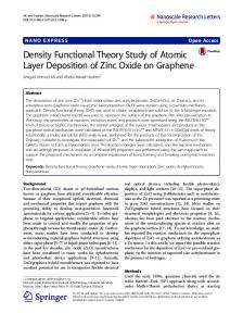
4. PROPOSED COMPUTATIONAL SETUP Given a nanostructure the goal is to determine the electron density distribution as well as the positions of the nuclei, that is, the mapping �. Here we do not consider dynamics of the nuclei. As indicated in Figure 2, the proposed computational approach has three principal modules: the preprocessing stage, the electronic problem and the ionic problem. Preprocessing is carried out once at the beginning of the simulation. A domain D0 is selected to include the nanostructure investigated. The partitioning of D0 into u subdomains Di � i = 1� � � � � u, is done to mirror the underlying periodicity of the structure. The subdomains D?�1� through D?�p� become the active subdomains and, as in Figure 1, they are denoted by Y1 through Yp . A set of values of the electron density is required at the nodes of the discretization mesh; the initial guess for the electron density could be an overlap of isolated atom electron densities throughout the nanostructure or, when practical, could be obtained based on periodic boundary conditions assumption by computing it in a domain Dj and then cloning for the remaining domains Dk . Preprocessing concludes with the initialization of the deformation map � to identity. With a suitable norm, the new electron density �new is compared to �init , and the computation restarts the electronic problem after setting �init = �new unless the corrected and initial values of the electron density are close. This iterative process constitutes the first inner loop of the algorithm. The ionic problem uses the newly computed electron density to reposition the nuclei. The nonlinear system in Eq. (3) provides the position of the repnuclei; the other nuclei are positioned based on the quasicontinuum paradigm according to Eq. (1). The nonlinear system is solved by an iterative method that leads to the second inner loop, which has four steps: 8
ELECTRONIC PROBLEM
ρ init = ρ new
ρ new− ρ init < ε? Only if nuclei positions change Reposition nuclei based on ρnew
IONIC PROBLEM
Reevaluate deformation mapping Φ Fig. 2. Computational flow. Proposed approach has three stage; an iterative loop spans the last two stages: the Electronic and Ionic Problems.
(a) evaluate the integral of Eq. (3); when necessary, evaluate its partial with respect to Pi ; (b) evaluate the double sum of Eq. (3), which is based on a partitioning of the structure, and, when necessary, evaluate its partial derivative with respect to the position of the representative atoms; (c) carry out a quasi-Newton step to update the positions Pi of the Mrep representative nuclei; and (d) go back to (a) if no convergence results. The precision in determining the positions of the nuclei is directly influenced by the accuracy of the electron density ��r�. Thus, an important issue, not addressed by this work, is the sensitivity of the solution of the nonlinear system in Eq. (3) with respect to ��r�. It remains to be determined what level of approximation of the electron density suffices for solving the ionic problem at a satisfactory level of accuracy. After determining the position of the nuclei, the algorithm computes the new deformation J. Nanosci. Nanotechnol. 8, 1–12, 2007
Negrut et al.
Quasicontinuum-Like Reduction of DFT Calculations of Nanostructures
mapping � according to Eq. (1). If the overall change in the position of repnuclei at the end of the ionic problem is smaller than a threshold value, the computation stops; otherwise the new distribution of the nuclei is the input to a new electronic problem (second stage of the algorithm). In summary, the algorithm passes through the preprocessing stage once. It then solves the electronic problem (the first inner loop) and proceeds to the ionic problem (the second inner loop). The outer loop (electronic problem, followed by ionic problem) stops when there is no significant change in the position of the repnuclei.
5. PRELIMINARY NUMERICAL RESULTS The fact that quasicontinuum method represents a meaningful reduction model approach has already been established.10–12� 24 The focus of the numerical experiments presented here is on model reduction as applied to the electronic problem. The approach proposed for the solution of the electronic problem has been investigated in the context of undeformed topologies. In other words, for the deformation gradient 0 ��r0 � t�, J �r0 � t� = det� 0 ��r0 � t�� = 1. 5.1. String of Atoms Example
(a) Relative error for 13/7 (245)
(b) Relative error for 13/5 (221) Fig. 3. Relative error surface for the 13-subdomain scenarios using (a) 7 and (b) 5 active subdomains. In parentheses we show the number of optimization iterations. The number of active subdomains considered in the algorithm reflects in the quality of the numerical solution: more active subdomains result in a larger number of degrees of freedom, which positively impacts ability to relax to lower energy levels and reduces boundary artifacts.
J. Nanosci. Nanotechnol. 8, 1–12, 2007
9
RESEARCH ARTICLE
Our first example is a three-dimensional variation of the one dimensional case analyzed in the previous section. The size of each of the 3D subdomains surrounding a hydrogen atom is 3 × 3 × 3 (all units henceforth are atomic
units). A full simulation with no reconstruction is provided as the reference solution. Two scenarios with seven and five active subdomains were subsequently considered; all meshes in this numerical experiment are uniform. In the first scenario, the subdomains D1 , D2 , D3 , D7 , D11 , D12 , and D13 were active; only D3 , D7 , and D11 were used for reconstruction. In the second scenario, the subdomains D1 , D2 , D7 , D12 , and D13 were active; only D2 , D7 , and D12 were used for reconstruction. For this test, the number of nodes/cells in the active subdomains is as follows: 28561/22464 for the nonreconstruction case (13/13), 15379/12096 for the 7/13, and 10985/8640 for the 5/13 case. All meshes considered herein, uniform or variable, are made up of hexahedrons. Figure 3 displays the relative errors; shown are only the regions where the relative error is larger than 5%. The results show a slight improvement in the seven-subdomain case; as the number of active subdomains increases, the quality of the results improve. Because of the dimension reduction, the size of the optimization problem decreases, thereby leading to a reduction in the number of iterations. Moreover, each iteration is computationally less expensive. The large relative errors are explained by the small values assumed by the electron density away from the nuclei where in practice it is expected to be zero. This and the boundary artifacts explain the accumulation of the 5% relative error isosurfaces far away from the nuclei and close to the boundary of the solution domain. While an exact quantitative characterization of the boundary artifacts remains to be produced, they are traced back to at least two sources. First,
Quasicontinuum-Like Reduction of DFT Calculations of Nanostructures
the small pockets of nonzero electron density are explained by a slow convergence rate of the optimization algorithm that currently does not use Hessian information and stops before clearing these pockets in remote corners of the nanostructure. Second, and more important, the assumption of underlying periodicity of the solution when used in conjunction with a small number of reconstruction subdomains (few degrees of freedom) limits the capacity of the electron density to relax due to these periodicity constraints that must be numerically satisfied. As expected and illustrated in the results corresponding to the 5 active subdomains case, the situation is exacerbated as fewer degrees of freedom are available in the energy minimization step of the method. In spite of these boundary artifact, it should be noted that the differences in total energy are small for both the 7 and 5 active subdomain cases (about 0.007%; see Table I). The results reported were obtained by running in parallel with 13 processes on a Linux cluster.
RESEARCH ARTICLE
5.2. Slab of Atoms Example Figure 4 shows the results obtained for the 5 × 5 subdomain 3D slab. Of the 25 subdomains considered for this simulation, one subdomain per nucleus of a hydrogen atom, only nine subdomains of darker color were considered active and used for reconstruction purposes. Figure 4(a) displays the electron density distribution on a mid-Z slice for the reconstructed domain (9/25). Figure 4(b) displays the subdomain structure of the slab, and Figure 4(c) shows the relative error produced through reconstruction. Compared to the reference case, the relative error in the total value of the electronic energy was 0.03%. The number of nodes/cells for the 5 × 5 case with all subdomains active was 33275/25000. For the 9/25 reconstruction scheme, the number of unknowns was reduced from 33275 to 11979. The 3D simulation was run in parallel using 25 processes on a Linux cluster.
Negrut et al.
(a) Electronic distribution for 25/25
D21
D22
D23
D24
D25
D16
D17
D18
D19
D20
D11
D12
D13
D14
D15
D6
D7
D8
D9
D10
D1
D2
D3
D4
D5
(b) Domain setup
5.3. Nonuniform Mesh Results Our third test investigated the effect of mesh adaptivity. An example consisting of a string of five hydrogen atoms was run in parallel on IBM BlueGene/L using five processes with no reconstruction. The solution on a uniform mesh is plotted in Figure 5(a); the variable mesh solution is presented in Figure 5(b). Although in both cases the number of mesh points is comparable, the total energy in the nonuniform case has a slightly smaller value, which Table I. Uniform mesh summary of the results. TAO-BLMVM optimization constraints are 10−6 for absolute and 10−5 for relative convergence tolerance. Active subdomains Number of iterations Total energy
10
13
7
5
605 −14.257
245 −14.256
221 −14.256
(c) Relative error for 9/25 Fig. 4. 5 × 5 three dimensional slab simulation scenario results. The reconstruction approach leads to good results in spite of topology dominated by large boundary to volume ratio.
indicates that it corresponds to a more relaxed distribution of the electron density. The peak electron density values are also higher for the variable mesh case because of a refined mesh capable of capturing fast variations in the vicinity of the nuclei. The energy values are slightly different in the two situations (a difference of 12%, from −5.8 to −5.2). In Figure 5 a “smearing” effect is noticed in the constant-size mesh, where the relatively higher values of the electron density occupy larger volumes but with lower peaks. Both simulations use the same optimization J. Nanosci. Nanotechnol. 8, 1–12, 2007
Negrut et al.
Quasicontinuum-Like Reduction of DFT Calculations of Nanostructures
13-atom example run with 7 active subdomains, the uniform mesh size scenario led to an energy of −14.257 in 245 iterations. The variable mesh case led to −15.54 in 3299 iterations, which is an order of magnitude increase in the number of iterations.
6. CONCLUSIONS
(a) Fixed mesh (– 5.1829/212)
Fig. 5. Density distribution for the 5-subdomain example using (a) a uniform mesh and (b) an adaptive mesh. Above each result we show the associated mesh. In parentheses we give the total energy/number of iterations. As anticipated, an adaptive mesh shows higher electron density peaks. Convergence speed if very slow though, and either Hessian information, or multigrid approach will have to be employed to address this issue.
settings (absolute and relative convergence tolerance). In each of the five subdomains, the number of nodes/cells was 10999/7712 for the variable mesh and 11661/9216 for the uniform mesh. The number of iterations in the nonuniform mesh case is much larger (2181 as opposed to 212). However, the nonuniform mesh results were obtained without using any acceleration strategy. The poor convergence speed can be addressed by a better mixing method,41� 42 multigrid approach and by providing Hessian information, which, while straightforward in the proposed approach, is not implemented yet. When one brings into the picture the reconstruction component, the trend noticed above persists. For the J. Nanosci. Nanotechnol. 8, 1–12, 2007
Acknowledgment: This work was supported in part by the Mathematical, Information, and Computational Sciences Division subprogram of the Office of Advanced Scientific Computing Research, Office of Science, and in part by the Office of Basic Energy Sciences-Materials Sciences, both under U.S. Department of Energy Contract 11
RESEARCH ARTICLE
(b) Nonuniform mesh (–5.8705/2181)
Density functional theory can accurately predict chemical and mechanical properties of nanostructures, although at a high computational cost. A quasicontinuum-like framework is proposed to substantially increase the size of the nanostructures accessible by simulations. The approach combines a model reduction paradigm and parallel computation capabilities to increase the size and reduce the simulation time associated with large simulations. The entire domain of interest is first meshed and divided into subdomains. The kinetic, exchange correlation, Coulomb, and electron-nuclei interaction energies are expressed in terms of grid values of the electron density in a subset of so-called active subdomains. The resulting form of the energy is minimized subject to the charge conservation constraint. The implementation leverages a domain-decomposition paradigm, and for parallel simulation support it builds on top of the MPICH2 library and the Toolkit for Advanced Optimization. One salient feature of the proposed approach is that the function and gradient evaluations, as well as the optimization stage, are run in parallel. The reconstruction errors were shown to depend on the extent of model reduction. For a test problem consisting of a three-dimensional string of one-electron atoms, the proposed approach led to a threefold reduction in the number of iterations for convergence, while maintaining small values of relative error for the total energy and the electron density in the regions of interest (boundary artifacts led to larger values in these boundary regions). The method could be improved in three ways. First, and most importantly, more advanced forms of the kinetic and exchange and correlation energy functionals need to be chosen, and the effective core potentials for many electron atoms have to be implemented. Second, for larger problems, cut-off techniques and fast-multipole methods43 need to be considered. These would ease memory limitations and allow the simulation of large reconstruction tests that go beyond the current proof-of-concept applications. Third, the reconstruction approach should be extended to the DFT Kohn-Sham approach because it has a significantly larger user base than OFDFT.
Quasicontinuum-Like Reduction of DFT Calculations of Nanostructures
No. DE-AC02-06CH11357. Emil Constantinescu and Toby Heyn are acknowledged for their support in generating the three-dimensional results reported in the paper, and we thank Nick Schafer for reading the manuscript and providing feedback. Use of computer resources from Argonne National Laboratory Computing Resource Center and US DOE National Energy Research Scientific Computing Center is gratefully acknowledged.
RESEARCH ARTICLE
References and Notes 1. W. Kohn and L. J. Sham, Phys. Rev. 140, A1133 (1965). 2. S. Goedecke and G. E. Scuseria, Computing in Science and Engineering 5, 14 (2003). 3. J. M. Soler, E. Artacho, J. D. Gale, A. Garcia, J. Junquera, P. Ordejón, and D. Sánchez-Portal, J. Phys.: Condens. Matt. 14, 2745 (2002). 4. C.-K. Skylaris, P. D. Haynes, A. A. Mostofi, and M. C. Payne, J. Chem. Phys. 122, 084119 (2005). 5. D. R. Bowler, R. Choudhury, M. J. Gillan, and T. Miyazaki, Phys. Stat. Sol. (b) 243, 989 (2006). 6. R. Santoprete, B. Koiller, R. B. Capaz, P. Kratzer, Q. K. K. Liu, and M. Scheffler, Phys. Rev. B 68, 235311 (2003). 7. O. Stier, M. Grundmann, and D. Bimberg, Phys. Rev. B 59, 5688 (1999). 8. L. W. Wang and A. Zunger, J. Phys. Chem. 98, 2158 (1994). 9. T. Kerdcharoen and K. Morokuma, Chem. Phys. Lett. 355, 257 (2002). 10. M. Fago, R. L. Hayes, E. A. Carter, and M. Ortiz, Phys. Rev. B70, 100102 (2004). 11. J. Knap and M. Ortiz, J. of the Mechanics and Physics of Solids 49, 1899 (2001). 12. E. Tadmor, M. Ortiz, and R. Phillips, Philosophical Magazine A 73, 1529 (1996). 13. P. Hohenberg and W. Kohn, Phys. Rev. 136, B864 (1964). 14. M. Levy and J. P. Perdew, Phys. Rev. A 32, 2010 (1985). 15. M. Anitescu, D. Negrut, T. Munson, and P. Zapol, Density Functional Theory-Based Nanostructure Investigation: Theoretical Considerations: Tech. Rep. ANL/MCS–P1252–0505, Argonne National Laboratory, Argonne, Illinois (2005). 16. J. Nocedal and S. J. Wright, Numerical Optimization, SpringerVerlag, New York (1999). 17. A. W. Appel, J. Sci. Stat. Comput. 6, 85 (1985).
Negrut et al.
18. L. Greengard, The Rapid Evaluation of Potential Fields in Particle Systems, MIT Press, Cambridge, Massachusets (1987). 19. H. G. Petersen, D. Soelvason, J. W. Perram, and E. R. Smith, J. Chem. Phys. 101, 8870 (1994). 20. L.-W. Wang and E. A. Carter, Theoretical Methods in Condensed Phase Chemistry Progress in Theoretical Chemistry and Physics, edited by S. D. Schwartz, Kluwer, Dordrecht (2000), pp. 117–184. 21. A. Aguado and J. M. Lopez, Phys. Rev. Lett. 94, 233401 (2005). 22. S. C. Watson and P. A. Madden, Phys. Chem. Comm. 1, 1 (1998). 23. R. Hayes, G. Ho, M. Ortiz, and E. Carter, Philos. Mag. 86, 2343 (2006). 24. R. E. Miller and E. B. Tadmor, J. Comput. Aided Mater. Des. 9, 203 (2002). 25. S. C. Watson and E. A. Carter, Comput. Phys. Commun. 128, 67 (2000). 26. W. Koch and M. C. Holthausen, A Chemist’s Guide to Density Functional Theory, John Wiley & Sons Inc., New York (2001), 2nd edn. 27. R. M. Martin, Electronic Structure: Basic Theory and Practical Methods, Cambridge University Press, Cambridge, U.K. (2004). 28. L. H. Thomas, Proc. Camb. Phil. Soc. 23, 542 (1927). 29. E. Fermi, Rend. Accad. Lincei 6, 602 (1927). 30. C. F. von Weizsacker, Z. Phys. 96, 431 (1935). 31. K. M. Carling and E. A. Carter, Modelling Simul. Mater. Sci. Eng. 11, 339 (2003). 32. M. Foley and P. A. Madden, Phys. Rev. B 53, 10589 (1996). 33. F. Perrot, J. Phys.: Condens. Matter 6, 431 (1994). 34. D. Negrut, M. Anitescu, T. Munson, and P. Zapol, Proceedings of IMECE 2005, ASME International Mechanical Engineering Congress and Exposition (2005). 35. M. Anitescu, D. Negrut, P. Zapol, and A. El-Azab, Mathematical Programming (2006). 36. N. Ashcroft and N. Mermin, Solid State Physics, W. B. Saunders Company, Philadelphia (1976). 37. Y. Kevrekidis, C. W. Gear, and J. Li, Phys. Lett. A 190 (2003). 38. D. Negrut, M. Anitescu, A. El-Azab, S. Benson, and P. Zapol, Journal of Computational Physics (2006). 39. S. J. Benson, L. C. McInnes, J. Moré, and J. Sarich, TAO User Manual (Revision 1.8): Tech. Rep. ANL/MCS-TM-242, Mathematics and Computer Science Division, Argonne National Laboratory (2005), http://www.mcs.anl.gov/tao 40. S. J. Benson, L. C. McInnes, and J. J. Moré, ACM Transactions on Mathematical Software 27, 361 (2001). 41. D. G. Anderson, J. Assoc. Comput. Mach. 12, 547 (1965). 42. C. G. Broyden, Math. Comput. 19, 577 (1965). 43. L. Greengard, Science 265, 909 (1994).
Received: 12 December 2006. Accepted: 26 February 2007.
12
J. Nanosci. Nanotechnol. 8, 1–12, 2007