the Fourier components of the dipolar field for large wave vectors. In this paper we ..... magnetization component mx perpendicular to the external field direction ...
PHYSICAL REVIEW B
VOLUME 57, NUMBER 22
1 JUNE 1998-II
Quasistatic remagnetization processes in two-dimensional systems with random on-site anisotropy and dipolar interaction: Numerical simulations D. V. Berkov and N. L. Gorn INNOVENT e.V., Go¨schwitzer Strasse 22, D-07745 Jena, Germany and Institute of Physical High Technologies, Helmholtzweg 4, D-07743 Jena, Germany ~Received 29 September 1997! We have developed a method that enables a fast and exact evaluation of the long-range interaction field by simulating the lattice dipolar systems with periodic boundary conditions. The method is based on the combination of the fast-Fourier-transformation technique and the modified Ewald method for the lattice sum calculation. We have used our algorithm for simulations of the quasistatic remagnetization processes in twodimensional hexagonal lattices of dipoles with the uniaxial on-site anisotropy ~anisotropic Heisenberg model with the long-range dipolar interaction!, which can be considered as a plausible model of a thin polycrystalline magnetic film with the intergrain exchange and with each crystallite having its own single-grain anisotropy. During the remagnetization process we observe typical ripplelike magnetization structures well known from the experimental observations. The parameters of these structures as functions of the exchange and anisotropy strength are studied. @S0163-1829~98!03522-X#
I. INTRODUCTION
Numerical simulation of strongly interacting manyparticle models is currently one of the most important tools for gaining information about a large variety of physical systems1 such as standard ferro- and antiferromagnetic Heisenberg models, exchange and dipolar spin glasses, and ferrofluids, among others.2,3 Micromagnetic simulations of equilibrium magnetization structures ~see, e.g., Refs. 4–7! and remagnetization dynamics in magnetic materials and thin films ~such as those performed in Refs. 8 and 9! can also be considered as simulations of many-particle models where one particle can be associated with a single cell arising from the discretization of a continuous problem. Among the systems listed above, those with the longrange interparticle interaction, mainly Ruderman-KittelKasuya-Yosida ~RRKY! or dipolar, are the most difficult to simulate for the obvious reason that the evaluation of an interaction field on each particle requires the summation of contributions from all other system particles. Thus the computer time for any algorithm using the straightforward summation grows as ;N 2 (N being a particle number!, so that using this simplest method only simulations for system having up to N;103 particles are possible even with modern supercomputers.10 The corresponding calculation can be greatly accelerated if we do not expect the formation of any long-range magnetization ~or polarization! structures such as magnetic domains. A good example of such a situation is the simulations of the quasistatic remagnetization processes in disordered systems without the strong nearest-neighbor exchange in a homogeneous external field.4,11,12 In this case only the field contribution from the particles in the so-called near zone ~i.e., from particles that are inside a sphere with the radius R rest around the given particle! should be calculated explicitly. The contributions from the rest of the system particles, i.e., from the particles outside this sphere, can be computed 0163-1829/98/57~22!/14332~12!/$15.00
57
as the Lorentz cavity field13 because on the large scale the magnetization is assumed to be homogeneous. The question how to choose the restriction radius R rest has to be solved separately in each concrete case, but in most applications4,12,14 it is sufficient to set this radius to be of the same order of magnitude as the mean interparticle distance. Thus only a small fraction of particles is contained in the near zone making the operation count for the interaction field evaluation proportional to ;nN, where the number of particles n in the near zone is n!N and, more importantly, independent of the system size. In such cases simulations for up to several thousand particles can be easily performed even with moderate computer facilities.4,12 The problem is much worse for the systems having both the strong nearest-neighbor exchange interaction and the relatively weak but long-range dipolar interaction. The interplay between these two forces may create complicated domain structures where the magnetization ~confining further discussion to magnetic systems! can be considered as homogeneous only on a very large length scale ~much larger than the average domain size!. This means that even methods using some artificial cutoff radius ~such as the Lorentz cavity method! would be extremely time consuming due to the very large value of this restriction radius required to obtain adequate results. Fortunately, for the lattice systems of this kind the methods using the fast-Fourier-transformation ~FFT! techniques for the dipolar field evaluation became available in the past decade.5,6,15 The methods are based on the observation that the dipolar field on the ith lattice site created by all other system moments
Hi 5
( jÞi
3ei j ~ ei j m j ! 2 m j r 3i j
~1!
can be rewritten as 14 332
© 1998 The American Physical Society
57
QUASISTATIC REMAGNETIZATION PROCESSES IN . . .
H ai 5
b ( W ab ij mj , b , jÞi
~2!
where a , b 5x,y,z, unit vectors ei j in Eq. ~1! are defined as ei j 5ri j /r i j , and the vectors ri j 5ri 2r j connect the cells i and j @we use the one-dimensional ~1D! notation for simplicity#. For the translationally invariant ~regular! lattice r i j depends on the site numbers i and j via their difference u i2 j u only, so the elements of the interaction matrices W ab ij also depend only on this difference. In this case the expression ~2! for the dipolar field components H ai 5
( ( W uabi2 j um bj jÞi b
~3!
can be recognized as an example of the discrete convolution. In Eq. ~3! the configuration of the magnetization components m bj plays the role of a signal and the interaction matrices W uab i2 j u can be viewed as the response functions in terms of the signal processing from where the whole formalism comes. Such a convolution is normally performed via the FFT using the corresponding theorem that under certain conditions ~see below! the Fourier transform of the field H ak is the dot product of the Fourier transforms of the interaction b coefficients W ab k and magnetic moments m k , H ak 5
b (b W ab k mk .
~4!
The major gain arises from the fact that the Fourier components of the magnetization can be evaluated all simultaneously in ;N ln N operations (N is the total number of lattice sites! using the FFT algorithm; the inverse Fourier transform from H ak to the field components in real space H ai 5H a (ri ) requires the same effort. Finally, the multiplication ~4! requires only ;N operations ~for N lattice sites we have N independent Fourier components!. Hence the evaluation of the dipolar field for all lattice sites can be performed in ;N ln N operations only, which ensures the nearly linear dependence of the calculation time on the particle number, almost as in systems with the short-range interaction. Using this idea, large-scale 2D and 3D micromagnetic simulations ~with the cell number N;105 ) have been performed.6,9,16 The implementation of this basically very simple idea meets, however, serious technical difficulties that are due to the conditions implied by the convolution theorem. The first condition formulated in terms of the signal processing theory requires that the signal should be a periodic function of time which in our case means the spatial periodicity of the magnetization configuration. The second condition requires that the response function should have a finite duration ~this is the counterpart of the requirement concerning the compactness of the kernel support in the convolution theorem for continuous functions! meaning for our situation that the interaction should be cut off at some finite distance. Both conditions are violated in the micromagnetic applications: ~i! The magnetization configuration is, generally speaking, not periodic and ~ii! the dipolar interaction is a long-range one and no physically reasonable cutoff radius can be introduced due to its quite slow decay (;r 23 ).
14 333
The conceptually simplest way to resolve these difficulties exists for the finite systems, i.e., ~i! magnetization configurations that are finite by themselves, such as small particles,16 or ~ii! those systems for which only their finite region creates the dipolar field, such as domain walls embedded in an infinite homogeneously magnetized medium6!. For such a finite system one can apply the zero padding technique, which is normally used in the signal processing to avoid aliasing due to the nonperiodicity of the signal. For the evaluation of the dipolar field the application of this technique means that we should first double the size of the initial lattice padding the magnetization configuration with zeros in all directions and second cut off the dipolar interaction matrices in Eq. ~3! at the distance equal to the size of the initial lattice. Then we can treat our system as a periodic magnetization configuration consisting of replicas of our initial system separated by areas of the same size having zero magnetization. There is no interaction between various replicas due to the cutoff of the dipolar matrices, so all physics of this artificial periodic configuration is still determined by the interaction inside one replica, as it was for the initial system. On the other hand, both conditions of the convolution theorem, the periodicity of the magnetization configuration and the finite range of the interaction, are fulfilled now and we can safely apply this theorem to evaluate the dipolar field.5,6,9 Important as they are, finite ~or, generally speaking, nonperiodic! magnetization configurations obviously do not cover the whole range of physically interesting problems. Simulations of magnetic systems with periodic boundary conditions are necessary, e.g., in classical micromagnetics, where periodic structures such as striped domains or bit structures arising in information storage media are important for various applications. Another very common situation where periodic systems appear are the Monte Carlo simulations of the thermodynamical properties for various lattice models, where periodic boundary conditions are almost unavoidable to reduce the influence of the finite-size effects.17 For systems with periodic boundary conditions the convolution theorem cannot be applied directly for the dipolar field calculations. The reason is that although the magnetization configuration is now periodic by the very definition of the periodic boundary conditions ~for, e.g., 3D problems the simulation region is supposed to be replicated infinitely many times in the x, y, and z directions!, the interaction between various replicas of the simulated system is essential ~in fact, this interaction is the main reason to use such boundary conditions at all! and hence the dipolar interaction cannot be truncated at any distance. This means that the second condition necessary for the application of the convolution theorem, the finite duration of the response function, is violated. In such cases one usually attempts to establish the connection between the Fourier components of the magnetization configuration and the dipolar field Hdip using the Poisson equation. This connection is then applied to calculate Hdip for any given periodical magnetization distribution. The method provides satisfactory results for the smooth magnetization changes along the lattice, but fails for the rapid mag-
14 334
D. V. BERKOV AND N. L. GORN
netization oscillations due to the ‘‘unpleasant’’ behavior of the Fourier components of the dipolar field for large wave vectors. In this paper we describe the modification of this method, which allows the rapid and exact calculation of the dipolar field for dipole lattices with periodic boundary conditions. Details of the method are given in Sec. II. The application of our method for the calculation of the quasistatic ~temperature T50) remagnetization processes in the 2D dipole system with the random uniaxial on-site anisotropy is described in Sec. III. In particular, this system is supposed to provide a reasonable model of polycrystalline magnetic thin films with uniaxial single-grain anisotropy when the anisotropy axes of the individual grains are distributed randomly in space. In Sec. IV results of our simulations are compared with experimental observations made during the remagnetization of such films. Further possible applications of our method are discussed in Sec. V. II. EVALUATION OF THE DEMAGNETIZING FIELD
To explain the principal difficulty arising from the Poisson equation method, we begin with the Poisson equation for the scalar magnetic potential D f ~ r! 524 pr ~ r! ,
~5!
where r (r) is the density of artificial ‘‘magnetic charges’’ defined via the magnetization M(r) as r (r)52¹M(r). The magnetic charge density of a single dipole m located at the point r can be expressed using the gradient of the corresponding d function as r (r)52 m¹ d (r).18 For a 2D N x 3N y lattice of magnetic dipoles the corresponding magnetic charge density is
(
i, j51
mi j ¹ d ~ ri 2ri j ! ,
~6!
where the lattice plane is chosen as the Oxy plane; in this plane lie the vector ri and vectors ri j that define the lattice node locations. For the sake of simplicity we also assume that magnetic dipoles have only x and y components ~oriented in the lattice plane! so that mi j 5 m xi j ex 1 m iyj ey . For such a lattice with periodic boundary conditions the charge density ~6! is also periodic in the Oxy plane; expanding mi j and d (ri 2ri j ) into a Fourier series and d (z) into a Fourier integral, we obtain the Fourier expansion of the charge density as
r ~ ri ,z ! 52 3
i 2 p DS
E
`
2`
dq z e iq z z
( @ m x~ q ! q x 1 m y ~ q ! q y # e iq –r ,
$ qi %
i
Applying the Laplace operator to this Fourier transform of the magnetic potential, substituting the result together with the expansion ~7! into the initial Poisson equation, and using the orthogonality properties of the Fourier harmonics on a finite lattice, we obtain the Fourier components of the magnetic potential as
f ~ qi ,q z ! 52
i
i
i
~7!
where DS is the area of one lattice cell in the Oxy plane, m x(y) (qi ) are the Fourier transforms of the dipole component arrays m x(y) i j , and the discrete sum is taken over the wave vectors corresponding to the lattice under consideration. The same Fourier transformation should be done for the magnetic potential ~expansion into the Fourier series in the Oxy plane and into the Fourier integral in the z direction!.
4 p i m x ~ qi ! q x 1 m y ~ qi ! q y • , DS q2
~8!
where q 2 5q2i 1q 2z . For further calculations we need the Fourier components of this potential in the Oxy plane, i.e., f (qi ,z50). They can be easily evaluated as
f ~ qi ,z50 ! 5
1 2p
E
`
2`
dq z f ~ qi ,q z ! ,
~9!
leading to the final result 2 p i m x ~ qi ! q x 1 m y ~ qi ! q y • f ~ qi ,z50 ! 52 . DS qi
~10!
In several applications, in particular, in numerical simulations using the ‘‘equation-of-motion’’ algorithms, the dipolar field Hdip itself ~rather than magnetic potential! is required. Fourier components of this field can be found using the standard relation Hdip52¹ f , which for the Fourier components reads H x (qi )52iq x f (qi ) and H y (qi )52iq y f (qi ), so that for the field Fourier components one finally obtains H x ~ qi ,z50 ! 52
2 p m x ~ qi ! q 2x 1 m y ~ qi ! q y q x • , DS qi
2 p m x ~ qi ! q x q y 1 m y ~ qi ! q 2y • H ~ qi ,z50 ! 52 . DS qi y
N x ,N y
r ~ r! [ r ~ ri ,z ! 52 d ~ z !
57
~11!
Note the difference between this result and the corresponding formulas for the stray field components used in Refs. 19 and 20 @i.e., Eq. ~6! in Ref. 20#. The formulas given in Refs. 19 and 20 are incorrect ~wrong power dependence on the wave vector components! which may be due to the absence of the d (z) function in the definition of the charge density in the papers cited above and the following absence of the integration ~9! over q z . The required stray field components at the lattice nodes H x (ri j ) and H y (ri j ) ~where magnetic moments are located! can now be obtained in the same way as by the application of the convolution theorem for finite systems, i.e., ~i! calculating the Fourier components m x(y) (qi ) of the magnetization arrays m x(y) via a FFT algorithm (;N ln N operations!, ~ii! ij multiplying them by the corresponding components of the wave vector qi to obtain the Fourier transform ~11! of the stray field H x(y) (qi ) (;N operations!, and ~iii! performing the inverse FFT to obtain the real space components of Hdip ~again ;N ln N operations!. The main problem when using this algorithm is due to the following two circumstances: First, for the finite lattice with the periodic boundary conditions we have at our disposal only a finite number of the Fourier components and, second, the Fourier components of the dipolar field ~11! do not, generally speaking, tend to zero for the large values of the wave
57
QUASISTATIC REMAGNETIZATION PROCESSES IN . . .
vector q ~they even diverge as ;q when q x ;q y ;q and q →`). The first circumstance forces us to cut off the Fourier spectrum of the dipolar field at the maximal wave vector components q x ;1/Dx and q y ;1/Dy, where Dx and Dy are the sizes of a single lattice cell. Due to the second circumstance this means a sharp ~abrupt! cut off of the Hdip Fourier spectrum, which may lead, as it is well known, to large artificial oscillations of the dipolar field. These oscillations can be observed very clearly if one tries to evaluate ~using the algorithm described above! the dipolar field of a single dipole placed somewhere on the lattice. In the classical micromagnetics this problem is often not very serious because the variation of the magnetization components along the lattice are quite slow due to the strong exchange interaction between the neighboring cells, i.e., both m xi j and m iyj are smooth functions of the node position (i, j). Hence their Fourier components for the large wave vectors (q x ;1/Dx, q y ;1/Dy) are very small thus leading to small Fourier components of Hdip @see Eq. ~11!#. In this case the cutoff of the Hdip Fourier spectrum at the maximal wave vectors available does not introduce any substantial oscillations because the spectrum components for these large q’s are already small by themselves. This is the reason why the direct evaluation of the dipolar field using the relations such as Eq. ~11! can provide satisfactory results ~see, e.g., Refs. 15 and 21!. However, in many systems such a ‘‘pleasant’’ behavior of the magnetization components ~their smooth variation! is clearly not the case. For example, even in classical micromagnetics rapid changes of the magnetization between the neighboring cells are possible if polycrystalline samples with the weakened exchange across the grain boundaries are simulated ~see, e.g., Refs. 7 and 19!. The problem is always present also in the Monte Carlo simulations of the thermodynamical properties of various lattice models22,23 where differences between the magnetic moments on the adjacent lattice sites are large at least above the ordering temperature. In these examples the error resulting from the sharp cutoff of the field spectrum is uncontrollable and hence some methods to resolve this difficulty are clearly needed. One obvious way to avoid the problem of the rapid field oscillations resulting from the abrupt magnetization changes along the lattice is to introduce some artificial magnetization variation inside a single cell ~i.e., to mimic the magnetization behavior in nature!. This is equivalent to the enhancement of the lattice spatial resolution and obviously removes the artificial field oscillation mentioned above because much larger Fourier vectors are now available, for which the Fourier components of the magnetization tend to zero due to a smooth variation of the magnetization inside a single cell. Thus the problem is removed exactly for the same reason as described above for the system with the smooth magnetization changes along the initial lattice. However, the price to be paid for such a simple solution is the corresponding growth of the computational time and required computer memory due to the larger number of lattice sites resulting from the lattice refinement. For this reason we propose another method that enables exact calculation of the dipolar ~or any other long-range! field on finite lattice systems with the periodic boundary conditions without introducing any magnetization distribution
14 335
inside a single cell thus avoiding the increase of the computational time due to the lattice refinement. The method is based on the combination of the Poisson equation method explained above and the modified Ewald method that is normally applied for the evaluation of the Coulomb lattice sums.13,24 Following the basic idea of the Ewald method we add and subtract at each lattice node (i, j) ~which carries the dipole moment mi j ) an artificial ‘‘Gaussian dipole’’ with the charge density given by @here and below the d (z) dependences of the charge density are omitted for simplicity#
r i j ~ r! 52
1 ~ 2 p ! 3/2a 5
F
3exp 2
@~ x2x i j ! m xi j 1 ~ y2y i j ! m iyj #
~ r2ri j ! 2
2a 2
G
,
~12!
where the choice of the ‘‘dipole width’’ a will be discussed later. One can easily verify that the total dipole moment of the distribution ~12! is 2 mi j . After this operation the charge density of the system can be written as the sum of two parts
r ~ r! 5 r A ~ r! 1 r B ~ r! ,
~13!
where the first part N x ,N y
r A ~ r! 52 2
(
mi j ¹ d ~ r2ri j !
i, j51
N x ,N y
1
(
@~ x2x i j ! m xi j 1 ~ y2y i j ! m iyj #
~ 2 p ! 3/2a 5 i, j51
S
3exp 2
~ r2ri j ! 2
2a 2
D
~14!
contains the sum of the pointlike dipoles ~6! @r (r) of the initial system# and the contribution of the ‘‘negative’’ Gaussian dipoles given by Eq. ~12! and the second part
r B ~ r! 5
N x ,N y
1 ~2p! a
(
3/2 5 i, j51
S
3exp 2
@~ x2x i j ! m xi j 1 ~ y2y i j ! m iyj #
~ r2ri j ! 2
2a 2
D
~15!
represents the density of the ‘‘positive’’ Gaussian dipoles that is added to cancel the second sum in Eq. ~15!. The gain achieved by this transformation is the same as in the standard Ewald method.13,24 The total dipole moment of the first part r A (r) connected with each lattice site is zero because the total moment of the negative Gaussian dipole exactly compensates the pointlike dipole of the initial system at each lattice site. For this reason the field created by the first part of the charge density r A (r) associated with each lattice site rapidly tends to zero ~see below! and may be treated as a short-range interaction. On the other hand, the second part r B (r) of the charge density is relatively smooth ~it is described not by the pointlike dipoles but by the smooth Gaussian distribution at each lattice site!, so the field created by this part can be safely calculated using the Poisson equation technique ~see the corresponding arguments above!.
14 336
D. V. BERKOV AND N. L. GORN
More precisely, the field created by the first part of the magnetic charge density r A (r) associated with the lattice site (i, j) is H xA,i j ~ r! 5
F
3 ~ x2x i j !~ mi j Dri j ! ~ Dr i j !
2
A
5
2
mx
G F
~ Dr i j ! 3
f G ~ Dri j !
G
2 ~ x2x i j !~ mi j Dri j ! ~ Dr i j ! 2 exp 2 , p 2a 2 ~ Dr i j ! 2 a 3 ~16!
y H A,i j ~ r! 5
F
3 ~ y2y i j !~ mi j Dri j !
2
~ Dr i j !
A
5
2
my
G F
~ Dr i j ! 3
f G ~ Dri j !
G
2 ~ y2y i j !~ mi j Dri j ! ~ Dr i j ! 2 exp 2 , p 2a 2 ~ Dr i j ! 2 a 3 ~17!
where Dri j 5r2ri j and the function f G (r) is defined via the standard error function erf(x) as f G ~ r! 512erf
S D r
a A2
1
A
S D
2r r2 exp 2 2 . pa 2a
~18!
From Eqs. ~17! and ~18! it can be seen that the field created by a single lattice node decays for r@a as exp(2r2/2a) and hence by the evaluation of the dipole field H dip A due to the part A of the charge density only the contributions from several nearest neighbors of each cell ~i.e., from those for which Dr i j ;a) should be taken into account. This means that the H dip A evaluation takes ;N operations for the whole lattice. The field H dip B due to the second part of the charge density ~15! can be calculated exactly as it was done for the lattice of the pointlike dipoles @see Eqs. ~5!–~11!#. The result is that the Fourier components of H dip B can be obtained from the Fourier transform ~11! of the field created by the point dipoles by multiplying the components ~11! by the factors exp(2q2i a2/2). These factors assure that H dip B (qi ) tend to zero for large wave vectors so that the spectrum cutoff due to the finite number of the Fourier components used does not lead to any artificial field oscillations. The last methodical problem is the choice of the Gaussian dipole width a. From Eqs. ~17! and ~18! it can be seen that a should be chosen as small as possible to ensure rapid decay of the short-range field H dip A , so that by its calculation only the contributions from the few nearest neighbors could be taken into account. On the other hand, a should not be too small because otherwise the factors exp(2q2i a2/2) that should cause the decay of the large-q Fourier components of H dip B will be not sufficiently small even for the largest available y wave vector components q xmax;1/Dx and q max ;1/Dy. We found that the choice a5max(Dx,Dy) for which the contributions from the three nearest-neighbor shells have to be taken into account by the H dip A evaluation provides the optimal compromise between the calculation speed and accuracy.
57
III. NUMERICAL SIMULATIONS OF 2D HEXAGONAL LATTICE SYSTEMS
Using the method introduced above, we have performed numerical simulations of quasistatic remagnetization processes in a 2D system of magnetic moments located on the hexagonal lattice with lattice constant ~the nearest-neighbors distance! a hex and periodic boundary conditions. The system can be viewed as an anisotropic 2D Heisenberg model with the long-range ~in this case dipolar! interaction. It can also be treated as a plausible model of a thin polycrystalline magnetic film where each crystallite has its own magnetic anisotropy. In this case the hexagonal lattice is supposed to model the hexagonal structure of certain kinds of magnetic thin films.25,26 The total system energy includes the energy of magnetic moments in the external field E ext , the local anisotropy energy E an , the energy of the exchange interaction between the nearest neighbors E exch and the dipolar ~also called demagnetizing! interaction energy E dip : E tot5E ext1E an1E exch1E dip .
~19!
Keeping in mind that the magnitude m i of the magnetic moment at each lattice site is usually constant ~which is the case for a standard Heisenberg model and by the micromagnetical simulations when a material is supposed to be well below its Curie temperature!, it is convenient to introduce the unit vectors mi 5 mi / m i defining the direction of magnetic moments at the ith lattice site and express the energy as a function of the orientations of these vectors. In this notation the energy in the external field is E ext52
(i m i~ mi Hext i !
~20!
~here and below we use for simplicity the 1D notation to mark lattice nodes!; the external field Hext can be inhomoi geneous ~site dependent!. The local anisotropy energy is assumed to include the contributions from the random uniaxial anisotropy ~due, e.g., to statistical orientation of the anisotropy axes ni of various crystallites! and from the homogeneous uniaxial anisotropy ~which may arise due to some specific features of the film preparation process! along the x or y axis in the film plane: E an52
(i D ~i r !~ mi ni ! 2 2D ~x0~ y! ! (i m 2i,x~ y !.
~21!
Here the anisotropy constant D (r) characterizes the random i (0) anisotropy strength on the ith site and D x(y) are the constants of homogeneous anisotropy along the x(y) axis. Below we assume that all D’s are positive, which corresponds to the easy axis case. The exchange energy has the standard Heisenberg form E exch52
1 J ~m m ! 2 ^ i, j & i j i j
(
~22!
where the sum is taken over the nearest neighbors ^ i, j & and the exchange constants J i j may be also site dependent. The remaining energy contribution, the dipolar interaction energy, is evaluated as
57
QUASISTATIC REMAGNETIZATION PROCESSES IN . . .
E dip52
1 2
(i m i~ miHdip i !,
~23!
where x and y ~in-plane! components of the dipolar field Hdip are evaluated using the formalism described in Sec. II, and the z component is calculated as the demagnetizing field of a z thin film, i.e., H dip z 524 p ( m i /V c ) where V c is the volume of one lattice cell so that the quantity m zi /V c corresponds to the material magnetization M z used in classical phenomenological calculations. This simplified calculation method for the perpendicular dipolar field component provides a good approximation when the variation of the z component of the magnetic moments along the lattice is smooth, which was always the case in our simulations. If the 2D system described above is supposed to simulate the behavior of a thin magnetic film having a thickness d and consisting of closely packed hexagons with the side b, then parameters entering the energy expression ~20!–~23! can be related to the magnetic material parameters: saturation magnetization M s , exchange stiffness of the bulk material A, and random and homogeneous uniaxial anisotropy constants K (r) (0) and K x(y) . The only nontrivial step when deriving the corresponding formulas is the establishment of the relation between the Heisenberg exchange constants J and the material exchange stiffness A. This can be done most conveniently by assuming that the magnetization rotation in real films takes place mainly on the grain boundaries between the neighboring crystallites. This suggestion is also physically reasonable because the exchange interaction is usually weaker in the intergrain space due, e.g., to the enhanced concentration of nonmagnetic impurities there. Under this assumption, using the method proposed in Ref. 27 we obtain the relation J 5 k (Abd/ d ), where d is the intergrain boundary thickness and k (,1) denotes the exchange weakening in the intergrain space when compared to the bulk exchange in the ideal material. The remaining connection between the anisotropy constants reads D5KV c , where K’s are the usual material anisotropy constants ~in ergs/cm3 ) and V c 5(3 3/2/2)b 2 d is the volume of the hexagonal lattice cell. If we assume that all lattice sites carry equal magnetic moments ~meaning, in the thin film model, equal volumes V i 5V 0 and equal magnetizations M s of all grains!, then it is convenient to introduce the reduced field h5H/M s and express the total energy in V 0 M 2s units as E V 0 M 2s
52
1
~r! 2 (i ~ mi hext i ! 2 ( b i ~ m i ni ! 2 i
1 2 b ~x0~ y! ! 2 2
1 2
1
C i j ~ mi m j ! (i m 2i,x~ y !2 2 ^( i, j &
(i ~ mi hdip i !,
~24!
where the reduced anisotropy b 52D/M 2s V 0 52K/M 2s and exchange C i j 5J i j /M 2s V 0 constants are introduced. To simulate quasistatic ~for the system temperature T50! remagnetization processes in such a system we have performed the minimization of the energy ~24! as a function of the unit vector orientations mi in a given external field using
14 337
the relaxation method described in Ref. 6. For the hysteresis loop simulations ~results of which are described below! we started, as usual, from the large (h ext;10) field where the magnetization configuration was nearly saturated and decreased the field consequently by a small amount using the equilibrium configuration obtained for the previous value as a starting condition for the new one.
IV. RESULTS AND DISCUSSION
In this section we present results of our simulations of the remagnetization processes in 2D hexagonal lattice systems with the nearest-neighbor exchange and long-range dipolar interaction between magnetic moments. Specifically we consider our simulations as modeling the behavior of thin polycrystalline magnetic films with random anisotropy, keeping in mind possible comparisons of our results with experimental data and other numerical simulations performed on such films. The parameter set used in our simulations, which will be referred to as a standard set, corresponds to thin Co films and is as follows: the material saturation magnetization M s 51.43106 A/m (51400 G!; the bulk exchange constant A 510211 J/m (51026 erg/cm!; an easy axis anisotropy with the constant K (r) 543105 J/m3 (543106 erg/cm3 ) and anisotropy axes randomly distributed in three dimensions is assigned to each grain ~cell or magnetic moment!; the homogeneous anisotropy contribution ~when not stated otherwise! (0) is absent: K (0) x 5K y 50; the side of the ~hexagonal! grain b55 nm; and intergrain separation d 51 nm. Thus, for the cell number N x 3N y 51283256 used in most simulations the corresponding physical system size was L x 3L y 5 A3bN x 31.5bN y '1.131.9 m m ~we neglected in this estimate the intergrain separation!. Exchange weakening k on the grain boundaries and the film thickness d were varied to study the corresponding dependences of the film properties ~see below!. All simulations of the remagnetization processes were performed on the IBM Pentium PC 133 MHz with 32 MB RAM using a code written in FORTRAN. An average run for a complete hysteresis loop ~;40 values of the external field, ;23104 iterations or effective field evaluations totally! for a system size N x 3N y 51283256'33104 cells took about 10 h. A typical hysteresis loop obtained in our simulations is shown in Fig. 1 together with the gray-scale maps of the magnetization component m x perpendicular to the external field direction, which was chosen as the y axis. The formation of the ripplelike magnetization structure can be clearly seen already for the relatively large external field @Fig. 1~a!#. When the field is decreased in the direction opposite to the initial system saturation, this ripple structure continuously transforms into the so-called blocked structure @Fig.1~b!; see also Fig. 1~c!#, which shows the system state immediately before the irreversible magnetization jump. The blocked structure then disappears after the magnetization switching occurs in larger fields @Fig. 1~d!#. The most useful characteristics of a random magnetization pattern such as those shown in Fig. 1 is the correlation function ~CF! of the magnetization, in our case the 2D correlation function of the m x component
D. V. BERKOV AND N. L. GORN
14 338
57
FIG. 1. Simulated hysteresis loop obtained for the film thickness d510 nm and the exchange weakening on the grain boundaries k 50.1 together with the gray-scale maps of m x values corresponding to various fields as indicated in the figure. Gray-scale maps presented here and in Figs. 4 and 5 show 643128 cuts from 128 3256 lattices actually simulated.
G m ~ r! [G m ~ x,y ! [ ^ m x ~ 0 ! m x ~ r! & ,
~25!
where the averaging is performed over the whole sample. In Fig. 2 the m x pattern in the remanent magnetization state for the entire simulated sample N x 3N y 51283256 together with the contour map of its CF @Fig. 2~b!# is shown. Only the central part of the G m (r) function is presented (216 ,r x ,r y ,16, where the distance is measured in lattice nodes! because outside the drawn region the CF exhibits only small, statistically insignificant oscillations around zero. The longitudinal ~along the initial direction of the external field! G m (0,y) and transverse ~perpendicular! G m (x,0) cuts of this CF looks qualitatively different, as shown in Fig. 3, which is a well known feature of the ripple structure occurring due to the dipolar interaction of individual grains. We define the characteristic ripple wavelength l as the double distance from the coordinate origin to the first minimum of the longitudinal CF @Fig. 3~a!# and the transverse correlation length as the integral L t5
E
L x /2
0
G m ~ x,0! dx.
FIG. 2. Remanent magnetization state of a 1283256 lattice shown as the m x ~a! gray-scale map and ~b! the corresponding space correlation function G ( m ) (r)[G ( m ) (x,y) of m x values ~see the text for details!.
Variation of the exchange coupling strength between the neighboring grains. We have studied the system properties for the exchange weakening region from k 50 ~exchange decoupled grains! up to k 50.2. For larger k values the cor-
~26!
Such a definition of L t is chosen because for an exponentially decaying CF G m (x,0)5exp(2x/xc) it would give the natural value L t 5x c if the simulated area is so large that x c !L x . Important parameters of a thin film ~made from a given magnetic material! that can be changed without a great effort are the exchange weakening on the grain boundaries k and the film thickness d. Dependences of the system properties on these two parameters obtained in our simulations are discussed below.
FIG. 3. Typical ~a! longitudinal G(y)[G(0,y) and ~b! transverse G(x)[G(x,0) correlation functions of the m x magnetization components for the remanent magnetization state. The characteristic ripple wavelength l is defined as shown in the figure and for the definition of the transverse correlation length L t see Eq. ~26!. Here and in all other figures all distances are measured in lattice constant units.
57
QUASISTATIC REMAGNETIZATION PROCESSES IN . . .
FIG. 4. Remanent magnetization states shown as m x gray-scale maps for various exchange weakening constants k as indicated in the figure. The same realization of the random directions of the easy anisotropy axes was used for all k values.
relation length of the magnetization pattern was of the same order of magnitude as the sample size, so a reliable statistical estimate of the system properties was not possible due to the finite size effects. The remanent magnetization structure ~presented again as the m x gray-scale map! for various k values is shown in Fig. 4. The structure clearly becomes coarser for larger exchange coupling, which manifests itself in the corresponding dependences of the average ripple wavelength @Fig. 5~a!# and transverse correlation length @Fig. 5~b!#. The dependence of the most important parameters of the hysteresis loop, the reduced remanent magnetization j R 5 m y (h50)/ m max and the coercivity h c 5H c /M s , is shown y in Fig. 6. As it was already observed in previous studies,28–30, the remanence @Fig. 6~a!# increases monotonically with the exchange coupling strength ~the slight decrease observed for large k values is within the statistical errors and will not be discussed until more precise data become available!. However, the values of the remanence that we observe for small exchange coupling are much lower ~up to 3 times! than those reported in Refs. 28 and 29. The explanation of this discrepancy that we propose is the following. For small exchange coupling the main interaction between grains ~magnetic moments! is the dipolar one. Hence, to obtain correct values of the magnetization in the absence of the external field ~which is the remanence! it is crucially important to evaluate the interaction field exactly. As it was mentioned above, both the hierarchical method used in Ref. 29 and the cutoff of the dipolar interaction used in Ref. 28 lead to errors of '1% in the dipolar field evaluation, whereby our method with parameters described in Sec.
FIG. 5. Dependences of ~a! the ripple wavelength l and ~b! the transverse correlation length L t ~b! on the exchange weakening k . In this and the following figures statistical errors, where not shown, are smaller than the symbol size.
14 339
FIG. 6. Dependences of ~a! the reduced remanent magnetization j R and ~b! the coercivity h c ~b! on the exchange weakening k .
II provides an accuracy better than 1023 , which should lead to substantial improvement of the accuracy by the simulation of the equilibrium magnetization configuration in small and zero external fields. To check the effect of small additional errors made by the dipolar field evaluation we have performed separate calculations adding to the exact values of the dipolar field calculated by our method random errors with the Gaussian distribution and the dispersion 1%. Indeed we found that such small errors lead to drastic changes in the remanence, so that for k 50 ~exchange decoupled grains! the remanence value obtained this way was j R '0.65 instead of the correct value j R 50.26 obtained without adding artificial errors. We would like to point out that this observation does not mean that a relative error about ;0.01 by the stray field evaluation leads to such drastic result changes for any magnetic system and parameter set. However, these results demonstrate how important the exact evaluation of the demagnetizing field for a micromagnetic problem may be, especially if other interactions are absent ~as in the example given above, where the magnetization configuration for the exchange decoupled grains in the absence of the external field is calculated!. It is also the manifestation of the well known fact that an equilibrium magnetization configuration may be very ‘‘soft’’ so that increasing the computational accuracy by the field evaluation even from ;0.01 up to ;0.001 may lead to substantial changes in the final result. The dependence of the coercivity on the exchange interaction strength @Fig. 6~b!# is also in qualitative agreement with the results of previous numerical simulations28,29 apart from the slight increase of h c for small k values, which is almost within the statistical errors and will be discussed elsewhere. Here we would like to point out that, in contrast to the previous results,28,29 the decrease of the coercivity for large exchange interaction values is much more pronounced. It is well known that, in general, such a decrease can be explained by the formation of large exchange-coupled clusters of grains that leads to the averaging of the randomly directed anisotropy fields of various grains and hence to the large reduction of the effective anisotropy constant of such a cluster. This decrease of the anisotropy, in turn, leads to the decrease of the coercivity of the system. One possible reason why do we observe a much larger decrease of the coercivity with the growth of the exchange coupling is a much larger size of the system that we are able to treat using our FFT-Ewald technique. Namely, the system sizes considered in Ref. 28 (26330 grains! and in Ref. 29 ('40350 grains! are of the same order of magnitude as the
14 340
D. V. BERKOV AND N. L. GORN
FIG. 7. Remanent magnetization states shown as m x gray-scale maps for various film thicknesses d as indicated in the figure.
correlation lengths l and L t for large k values ~see Fig. 5!. This means that in the latter cases the coercivity could be determined by the finite size effects because effectively the reversal of ;1 cluster was considered. Another probable explanation for such a difference in the coercivity values could be again the higher precision in our stray field calculations because this field is also very important near the coercivity point where the magnetization variation ~and hence ‘‘magnetic charges’’ creating the stray field! is especially strong. Variation of the film thickness. To study the dependence of various system properties on the film thickness d we have performed simulations of the remagnetization processes for films with thicknesses from d min51 nm up to d max540 nm. Examples of the remanent magnetization structures for various thicknesses are shown in Fig. 7 ~again as the gray-scale maps of the m x component!. It can be clearly seen that for the smallest thickness studied (d51 nm! there are no ripple manifestations whatsoever and the magnetization pattern is completely isotropic, which can be verified plotting its 2D correlation function ~in this case only the decay correlation length L t can be defined!. The obvious reason is that for such a small thickness the magnetic moment of an individual grain is so small that intergrain interactions play almost no role so that the system behaves itself as an assembly of almost noninteracting single-domain particles having uniaxial anisotropy and the randomly distributed anisotropy axes. When the thickness is increased, the characteristic ripple structure starts to establish itself and the longitudinal ~along the external field direction! 1D correlation functions begin to resemble those shown in Fig. 3~a!; starting approximately from the thickness d54 nm, it is possible to define the average ripple wavelength. Thickness dependences of this average wavelength l and the transverse correlation length L t are presented in Fig. 8.
FIG. 8. Dependences of ~a! the ripple wavelength l and ~b! the transverse correlation length L t on the film thickness d.
57
The most characteristic feature of the dependences shown in Fig. 8 is the nonmonotonic behavior of both l and L t as functions of the film thickness d: They have a maximum around a value d510 nm @we note, however, that the maximum on the L t (d) dependence is almost within statistical errors#. Although we lack the complete explanation for such a behavior, we would like to present some qualitative speculations. The initial increase of both correlation lengths l and L t for small d’s is obviously due to the increasing strength of the intergrain interaction resulting from the increasing magnetic moment of a single cell; this leads to the establishment of a strong correlation between adjacent moments and to the formation of the ripple structure. After such a structure has been formed completely ~this happens for d'6 – 10 nm!, the dipolar and the exchange interactions begin to compete: ~i! The dipolar interaction tries to decrease the average ripple wavelength because the magnetostatic energy decreases when the charges of the opposite signs are drawn closer to each other and ~ii! the exchange interaction tends to avoid rapid changes in the magnetization direction, thus trying to increase the average wavelength. Both interaction fields scale with the film thickness as ;d, but the dipolar interaction is a long-range one and hence its strength increases faster ~the corresponding coefficient before the ;d dependence is larger! so that the average wavelength decreases with d after the ripple structure has been formed. Here some comments concerning the validity of the dipolar approximation used by the stray field evaluation are necessary. For the basic parameter set, where the film thickness is 10 nm and the cell size in the film plane is also '10 nm, this approximation is quite good ~because a single cell can be approximated reasonably by a sphere!. However, for much smaller and much larger film thicknesses this approximation clearly becomes poorer, so that results presented in Fig. 8 should be considered at best as semiquantitative if we have in mind the simulation of magnetic thin films. However, these results are exact if one would like to consider our computations as simulations of remagnetization processes in 2D dipolar lattices with constant lattice spacing by various dipole strengths ~because, in the dipolar approximation, varying the film thickness, we change only the magnitude of the dipole moment connecting with each cell!. Effect of the homogeneous uniaxial anisotropy. It is well known that some film preparation techniques lead to the induction of the ~usually weak! homogeneous uniaxial anisotropy. Hence it would be interesting to study the effect of such an anisotropy on the magnetization structure. Figure 9 demonstrates remanent magnetization states obtained by the simulation of the remagnetization processes in the films with a standard parameter set ~see above, in particular, k 50.1 and d510 nm! and the homogeneous uniaxial anisotropy with the easy axes directed as shown in the figure. The initial direction of the saturation field was chosen as usual along the y axis. The value of the homogeneous anisotropy constant is K (0) 553104 J/m3 (553105 ergs/ cm3 ), which is approximately 10 times smaller than the corresponding value of the anisotropy constant of the randomly directed single-grain anisotropy [K (r) 543105 J/m3 (54 3106 ergs/cm3 )]. Nevertheless, the effect of the homogeneous anisotropy can be clearly seen; as expected, the anisotropy directed along the ripple stripes ~perpendicular to the
57
QUASISTATIC REMAGNETIZATION PROCESSES IN . . .
FIG. 9. Remanent magnetization states shown as m x gray-scale maps (1283256 lattices! for various kinds of homogeneous anisotropy as shown in the figure. The homogeneous anisotropy constant for cases ~a! and ~c! is K ( 0 ) 553104 J/m3 (553105 ergs/cm3 ).
initial field direction! greatly enhances the contrast of the ripple structure. We expect that for larger exchange coupling even lower values of the homogeneous anisotropy can have a pronounced influence on the magnetization structure. Our results are in a qualitative agreement with the observations made by McCord.31 A comparison of our results with the existing ripple theories ~see Refs. 32 and 33 and references therein! is not very useful because most of them are built in the linear approximation, i.e., small magnetization deviations from the saturated state are assumed. The most qualitatively nontrivial prediction of such theories that can be related to our simulations is the calculation of the magnetization correlation function done by Maass.34 The shapes of the contour lines obtained in Ref. 34 agree qualitatively remarkably well with those shown in Fig. 2~b!. Results for the corresponding Green function ~which in this case behaves itself qualitatively similar to the correlation function! are presented in Ref. 35, which can be accessed much more easily. The only nonlinear ripple theory known to us36 ~which, according to Ref. 36, should be valid for permalloy films if the magnetization deviation angle does not exceed '20°) predicts the growth of the ripple correlation length with the exchange constant ~however, only a linear growth! and does not predict any nonmonotonic behavior of the correlation lengths as functions of the film thickness. For the experimental verification of the results of our simulations the observation of the magnetic structures during the remagnetization process with the resolution of at least several hundreds of nanometers is necessary. From the experimental images the correlation functions such as Eq. ~25! could be obtained to compare corresponding correlation lengths with our results. Independent measurements of the exchange coupling between grains and the film thickness would be necessary. Whereby the latter could be performed relatively straightforward, estimations of the exchange coupling could be done using the values of the remanence and coercivity obtained from the hysteresis loops. There are currently two groups of methods that possess the necessary spatial resolution: magnetic force microscopy ~MFM! and Lorentz microscopy. High-resolution measurements using MFM can be found, e.g., in Ref. 37, where it is shown that the polycrystalline film with the lowest coercivity exhibited the coarsest magnetic microstructure ~i.e., the larg-
14 341
est correlation length!, which is qualitatively consistent with our results. A good example of the Lorentz microscopy images is given in Ref. 38, where the magnetic microstructure of the thin CoCr films was investigated. Images presented there are qualitatively very similar to those observed in our simulations, but again no quantitative comparison can be made. We also would like to make some comments concerning the comparison of our method for the dipolar field evaluation with other proposed algorithms15,19,20,28,29,39,40 ~the advantages of our method when compared with the techniques based on the increasing number of the Fourier components20 are explained in Sec. II!. First of all, some authors28,39,41 propose to truncate the dipolar interaction taking into account only contributions from the finite number of nearest neighbors, thus reducing the operation count for the dipolar field evaluation formally to ;N ~we recall that in our method the corresponding dependence is ;NlnN). Although formally possible for 2D problems, this trick does not help very much because, due to the quite slow decay of the dipolar interaction (;r 23 ), a large number of nearest neighbors, typically several hundreds,28,39,41 should be taken into account to achieve a reasonable accuracy. Hence the proportionality factor in the ;N dependence of the operation count is so large that for the cell numbers N currently available the FFT method turns out to be faster. Another drawback of the truncation method is that for each set of system parameters the truncation radius should, strictly speaking, be determined separately by performing simulations with an increasing number of nearest neighbors taken into account. The last ~but not the least! problem is that this method cannot be applied to 3D problems, whereas our FFT-Ewald algorithm can be easily generalized for this case. The next method that allows large-scale micromagnetic simulations including the dipolar field effects is the hierarchical model developed by Miles and Middleton.29 The model is based on ~i! the explicit summation of the dipolar field contributions over a ~relatively small! number of nearest neighbors and ~ii! summation of the contributions from the far zones divided into larger cell blocks. The algorithm also has the operation count ;NlnN and an adequate choice of block sizes and structure enables us to make the dipolar field calculation errors ~arising from the moment averaging inside large blocks! reasonably small. The major problems in this method are the relatively complicated algorithm implementation, the choice of the parameters of the hierarchical block structure, and the error estimation, which ~as for the truncation methods! should be performed separately for each new set of system parameters. This is not the case in our algorithm, which is simple to handle and for which the error ~arising only from the truncation of the short-range field H dip A ) can be estimated in advance. As mentioned above, it turned out to be vanishingly small already for two ~in the worst case three! nearest-neighbor shells taken into account. Another question when applying the hierarchical model is how to take correctly into account periodic boundary conditions. However, it should be pointed out that both groups of methods discussed above ~truncation and the hierarchical model! are able to simulate disordered structures, which is not possible for our technique because the Fourier expansion
14 342
D. V. BERKOV AND N. L. GORN
requires the translational invariance of the lattice. We can account for any type of randomness @random anisotropy, random distribution of the intergrain exchange coupling, distribution of the saturation magnetization ~magnetic moments! among the lattice sites, etc.# except for the structural disorder. The introduction of such a disorder is believed to be necessary for simulating real thin films because in some cases it clearly influences the macroscopic magnetic properties of the system.39,40 However, the question whether the same effect can be produced using a regular lattice with the statistical distribution of another parameters mentioned above is ~to our knowledge! still not sufficiently studied. Another important and quickly developing area where our algorithm for the dipolar field evaluation can be used is the simulation of the equilibrium and nonequilibrium thermodynamics of various 2D lattice systems,2,42 which for the models with the long-range interactions are still performed for moderate lattice sizes only.22,23,43 It should be clear that our method is not suitable for the Metropolis-type algorithms used for the simulation of equilibrium thermodynamical properties where single-moment updates are performed because the great acceleration by the dipolar field evaluation (;N ln N instead of ;N 2 ) is achieved only when this field is evaluated simultaneously on all lattice sites. Hence, to take advantage of this acceleration an algorithm based on the Langevin dynamics of the system should be used.44,45 Due to
1
Monte Carlo Method in Statistical Physics, edited by K. Binder ~Springer-Verlag, Berlin, 1987!; Monte Carlo Method in Condensed Matter Physics, edited by K. Binder ~Springer-Verlag, Berlin, 1995!. 2 K. Binder and A. P. Young, Rev. Mod. Phys. 58, 801 ~1986!. 3 Proceedings of the International Workshop on Magnetic Properties of Fine Particles, Rome, 1991, edited by J. L. Dormann and D. Fiorani ~North-Holland, Amsterdam, 1992!. 4 M. J. Vos, R. L. Brott, J. Zhu, and L. W. Carlson, IEEE Trans. Magn. MAG-29, 3652 ~1993!. 5 S. W. Yuan and H. N. Bertram, IEEE Trans. Magn. MAG-28, 2031 ~1992!. 6 D. V. Berkov, K. Ramstoeck, and A. Hubert, Phys. Status Solidi A 137, 207 ~1993!. 7 T. Schrefl, J. Fidler, and H. Kronmueller, Phys. Rev. B 49, 6100 ~1994!. 8 Y. Nakatani and Y. Uesaka, Jpn. J. Appl. Phys., Part 1 28, 2485 ~1989!. 9 S. W. Yuan and H. Bertram, Phys. Rev. B 44, 12 395 ~1991!. 10 D. Wei, H. N. Bertram, A. Friedmann, and R. H. Dee, IEEE Trans. Magn. 31, 2898 ~1995!. 11 Y. Zhao and H. N. Bertram, J. Magn. Magn. Mater. 114, 329 ~1992!. 12 D. V. Berkov, J. Magn. Magn. Mater. 161, 337 ~1996!. 13 C. Kittel, Introduction to Solid State Physics ~Wiley, New York, 1953!. 14 M. Faehnle, Appl. Phys. 20, 275 ~1979!. 15 M. Mansuripur and R. Giles, IEEE Trans. Magn. MAG-24, 2326 ~1989!. 16 K. Fabian, A. Kirchner, W. Williams, F. Heider, and A. Hubert, Geophys. J. Int. 124, 89 ~1996!.
57
the nearly linear computational time dependence on the lattice site number almost the same performance as by the simulations of the short-range models42 is expected. It should also be mentioned that the transfer of our method on other long-range interaction types such as the RKKY interaction is straightforward. V. CONCLUSION
We have presented a method for the evaluation of the long-range dipolar interaction fields in lattice systems with periodic boundary condition. Using this method, we were able to perform large-scale numerical simulations of the quasistatic remagnetization processes in 2D dipolar systems with random on-site anisotropy and nearest-neighbor exchange interaction. A couple of results concerning the dependence of the hysteresis loop parameters and the magnetization correlation lengths were presented. The applicability of our method to the simulations of equilibrium and nonequilibrium thermodynamics of lattice systems with long-range interaction was discussed. ACKNOWLEDGMENTS
The authors are greatly indebted to Professor W. Andra¨ and Dr. R. Mattheis for many useful discussions.
17
K. Binder and D. W. Heerman, Monte Carlo Simulation in Statistical Physics ~Springer-Verlag, Berlin, 1992!. 18 L. D. Landau and E. M. Lifshitz, The Classical Theory of Fields ~Pergamon Press, Oxford, 1975!. 19 M. Mansuripur and R. C. Giles, Comput. Phys. 4, 291 ~1990!. 20 R. C. Giles, P. R. Kotiuga, and M. Mansuripur, IEEE Trans. Magn. MAG-27, 3815 ~1991!. 21 L. I. Antonov, V. V. Ternovskij, and M. M. Khapaev, Fiz. Met. Metalloved. 67, 52 ~1989!. 22 A. Hucht, A. Moschel, and K. D. Usadel, J. Magn. Magn. Mater. 148, 32 ~1995!. 23 S. T. Chui, J. Appl. Phys. 79, 4951 ~1996!; J. Magn. Magn. Mater. 168, 9 ~1997!. 24 J. C. Slater, Insulators, Semiconductors and Metals ~McGrawHill, New York, 1967!. 25 T. Chen and T. Yamashita, IEEE Trans. Magn. MAG-24, 2700 ~1988!. 26 W. Andra¨, H. Danan, and R. Mattheis, Phys. Status Solidi A 125, 9 ~1991!. 27 C. Kittel, Rev. Mod. Phys. 21, 541 ~1949!. 28 J.-G. Zhu and H. N. Bertram, J. Appl. Phys. 63, 3248 ~1988!. 29 J. J. Miles and B. K. Middleton, J. Magn. Magn. Mater. 95, 99 ~1991!. 30 J. J. Miles, M. Wdowin, and B. K. Middleton, IEEE Trans. Magn. MAG-31, 1013 ~1995!. 31 J. McCord ~private communication!. 32 W. F. Brown, IEEE Trans. Magn. MAG-6, 121 ~1970!. 33 K. J. Harte, MIT Lincoln Laboratory Report No. DS-5242, 1967 ~unpublished!. 34 W. Maass, Ph.D. thesis, University of Regensburg, 1984.
57 35
QUASISTATIC REMAGNETIZATION PROCESSES IN . . .
W. Maass, U. Krey, and H. Hoffmann, J. Magn. Magn. Mater. 37, 11 ~1983!. 36 K. J. Harte, J. Appl. Phys. 37, 1295 ~1966!. 37 P. Glijer, J. M. Silvertsen, and J. H. Judy, IEEE Trans. Magn. MAG-31, 2842 ~1995!. 38 P. ten Berge, J. C. Lodder, R. Plo¨ssl, and J. N. Chapman, J. Magn. Magn. Mater. 120, 362 ~1993!. 39 J. J. Miles and B. K. Middleton, IEEE Trans. Magn. MAG-26, 2137 ~1990!. 40 J. J. Miles and B. K. Middleton, IEEE Trans. Magn. MAG-31,
14 343
2770 ~1995!. J.-G. Zhu and H. N. Bertram, IEEE Trans. Magn. MAG-24, 2706 ~1988!. 42 D. P. Landau, Physica A 205, 41 ~1994!. 43 S. T. Chui, Phys. Rev. B 50, 12 559 ~1994!; Phys. Rev. Lett. 74, 3896 ~1995!. 44 J. M. Sancho and A. M. Lacasta, Phys. Lett. A 181, 335 ~1993!. 45 A. Lyberatos, D. V. Berkov, and R. W. Chantrell, J. Phys.: Condens. Matter 5, 8911 ~1993!. 41


![QUASISTATIC PROCESSES FOR [15]](https://m.moam.info/img/260x300/quasistatic-processes-for-15_5c5285d3097c47113c8b45af.jpg)