Query Dependent Ranking Using K-Nearest Neighbor∗ Xiubo Geng *
Tie-Yan Liu
Institue of Computing Technology Chinese Academy of Sciences Beijing, 100190 P.R. China
Microsoft Research Asia No.49 Zhichun Road, Haidian District Beijing 100190, P.R. China
Machine Learning Department Carnegie Mellon University Pittsburgh,PA 15213, USA
Microsoft Research Asia No.49 Zhichun Road, Haidian District Beijing 100190, P.R. China
[email protected] Andrew Arnold *
[email protected]
[email protected] Hang Li
Tao Qin *
Dept. Electronic Engineering Tsinghua University Beijing, 100084, P.R. China
[email protected]
Heung-Yeung Shum
Microsoft Corporation Redmond,WA 98115, USA
[email protected]
[email protected]
ABSTRACT Many ranking models have been proposed in information retrieval, and recently machine learning techniques have also been applied to ranking model construction. Most of the existing methods do not take into consideration the fact that significant differences exist between queries, and only resort to a single function in ranking of documents. In this paper, we argue that it is necessary to employ different ranking models for different queries and conduct what we call query-dependent ranking. As the first such attempt, we propose a K-Nearest Neighbor (KNN) method for querydependent ranking. We first consider an online method which creates a ranking model for a given query by using the labeled neighbors of the query in the query feature space and then rank the documents with respect to the query using the created model. Next, we give two offline approximations of the method, which create the ranking models in advance to enhance the efficiency of ranking. And we prove a theory which indicates that the approximations are accurate in terms of difference in loss of prediction, if the learning algorithm used is stable with respect to minor changes in training examples. Our experimental results show that the proposed online and offline methods both outperform the baseline method of using a single ranking function.
Categories and Subject Descriptors H.3.3 [Information Search and Retrieval]: Retrieval models
General Terms Algorithms, Performance, Experimentation ∗The work was done when the first, the third, and fourth authors were interns at Microsoft Research Asia.
Permission to make digital or hard copies of all or part of this work for personal or classroom use is granted without fee provided that copies are not made or distributed for profit or commercial advantage and that copies bear this notice and the full citation on the first page. To copy otherwise, to republish, to post on servers or to redistribute to lists, requires prior specific permission and/or a fee. SIGIR’08, July 20–24, 2008, Singapore. Copyright 2008 ACM 978-1-60558-164-4/08/07 ...$5.00.
Keywords Query dependent ranking, k-nearest neighbor, stability
1. INTRODUCTION Ranking will continually be an important research topic, as long as search and other information retrieval applications keep developing and growing. When used in search, ranking becomes a task as follows. Given a query, the documents related to the query in the document repository are sorted according to their relevance to the query using a ranking model, and a list of top ranked documents is presented to the user. The key problem for the related research is to develop a ranking model that best represents relevance. Many models have been proposed for ranking, such as the Boolean model [2], the vector space model [23, 24], BM25 [21] and language model for IR [13, 18]. Recently, machine learning techniques called learning to rank have also been applied to automatic ranking model construction [5, 6, 7, 11, 17]. By leveraging labeled training data and machine learning algorithms, this approach is able to make the tuning of ranking model theoretically sounder and practically more effective. The training data consists of queries, their associated documents and labels representing relevance of documents. In this paper, we also base our work on learning to rank. In most of the previous work, a single ranking function is used to handle all queries. This may not be appropriate, particularly for web search, as explained below. Instead, it would be better to exploit different ranking models for different queries. In this paper, we refer to this approach as query-dependent ranking. (We note that some authors use the term ‘query dependent ranking’ to refer to the document ranking process of using both query information and document information, in contrast to the process of using document information alone [20]. We use the term differently in this paper.) Queries in web search may vary largely in semantics and the users’ intensions they represent, in forms they appear, and in numbers of relevant documents they have in the document repository. For example, queries can be navigational, informational, or transactional [22]. Queries can be personal names, product names, or terminology. Queries can be phrases, combinations of phrases, or natural language sentences. Queries can be short or long. Queries can be popular (which have many relevant documents) or rare (which only have a few relevant documents). Using a single model alone would make compromises among the cases and result in lower accuracy in relevance ranking.
The IR community has realized the necessity of conducting querydependent ranking. However, efforts were mainly made on query classification [3, 4, 12, 14, 22, 25, 26], but not ranking model construction or ranking model learning. The only exception is Kang and Kim’s work [12], to our knowledge, in which queries were classified into two categories based on search intension and two different ranking models were tuned and used for the two categories. Therefore, more investigations on the approach are needed, which is also the motivation of this work. Inspired by previous work [8], we propose a query-dependent method for ranking model construction, on the basis of K-Nearest Neighbor (KNN). We position the training queries into the query feature space in which each query is represented by a point. In ranking, given a test query we retrieve its k nearest training queries, learn a ranking model with these training queries, and then rank the documents associated with the test query using that model. The accuracy of ranking can be enhanced by employing the proposed method, due to the following reasons. First, in the method ranking for a query is conducted by leveraging the useful information of the similar queries and avoiding the negative effects from the dissimilar ones. Second, ‘soft’ classification of queries is carried out and similar queries are selected dynamically. Our experimental study has verified the superiority of the KNN method to both the single model approach and the query classification based approach. Since KNN needs to conduct online training of the ranking model for each test query, and this would not be affordable in practice, we further propose two approximations of the method, which move the training offline. We give both theoretical justification and empirical verification for the two offline methods. Specifically, we prove that the approximations are accurate in terms of difference in loss of prediction, if the learning algorithm used is stable with respect to minor changes in training examples. The contributions of this paper include the following points: (1) Proposal of the approach of query-dependent ranking, (2) Development of KNN methods for query-dependent ranking, (3) Theoretical and empirical investigations of the methods. The rest of this paper is organized as follows. In Section 2, related work is presented. In Section 3, the KNN method for querydependent ranking is proposed. In Section 4, experimental results are reported. In the last section, conclusions are made and future work is discussed.
2.
RELATED WORK
There has not been much previous work on query dependent ranking, except [12], as explained above. The most relevant research topics are query classification and learning to rank. Many efforts have been made on query classification. In [3, 4, 25], queries were classified according to topics, for instance, Computers, Entertainment, Information, etc. as used in KDD Cup 2005. In [12, 14, 22, 26], queries were classified according to users’ search needs, for instance, topic distillation, named page finding, and homepage finding. Machine learning methods such as support vector machines were usually employed in the classification. However, query classification was not extensively applied to query dependent ranking, probably due to the difficulty of the query classification problem. Recently, a large number of studies have been conducted on learning to rank and its application to information retrieval. Existing methods for learning to rank fall into three categories: the pointwise approach [17], which transforms ranking to classification or
4
2
0
−2
−4 Named page finding Homepage finding Topic distillation
−6
−8 −4
−2
0
2
4
6
8
10
Figure 1: Distribution of Queries in TREC 2004 Data. regression on single documents; the pair-wise approach [5, 7, 11], which formalizes ranking as classification on document pairs; and the list-wise approach [6, 28, 29], which directly minimizes a loss function defined on document lists. The KNN based method proposed in this paper can also be viewed as a new learning to rank method.
3. RANKING USING K-NEAREST NEIGHBOR 3.1 Motivation Queries can vary greatly between each other in several perspectives, as explained above. For example, popular queries like ‘soccer’ can have many relevant documents and thus features measuring document popularity (e.g. PageRank) will be important for ranking the documents related to this query. In contrast, rare queries like ‘SIGIR 2007 workshop on learning to rank’ may only have a few relevant documents, and thus the use of document popularity in ranking is not even necessary. Using a single ranking model alone would not be able to deal with these cases properly. Naturally we think about employing the ‘query dependent approach’, in which we train and use different ranking models for different queries. A straightforward approach to query dependent ranking would be to employ a ‘hard’ classification approach in which we classify queries into categories and train a ranking model for each category. We think, however, that it could be very difficult to achieve high performance with this approach . When looking at the data, we often observe that it is hard to draw clear boundaries between the queries in different categories. Let us take the TREC 2004 web track data as an example. There are in total 225 queries in the dataset, which have been manually classified into three categories: topic distillation, named page finding, and homepage finding. The queries are also associated with documents and relevance labels of these documents. We define features of queries, following the proposal in [26], and represent the queries in a 27-dimensional query feature space. We next reduce the space to 2-dimensions by using Principal Component Analysis (PCA). We then plot the queries in this reduced space and obtain the graph in Figure 1. One can see from the figure that queries in different categories are mixed together and cannot be separated using hard classification boundaries. At the same time, one can observe that with high
Algorithm: KNN Online Input: neighbors of q, which are used to learn a model for q
(1) A test query q and the associated documents to be ranked. (2) Training data {S qi , i = 1, ..., m}. (3) Reference model hr (currently BM25). (4) Number of nearest neighbors k. Output: Ranked list for query q.
test query q
Figure 2: Illustration of KNN Online.
Algorithm: Offline pre-processing: For each training query qi , use reference model hr to find its top T ranked documents, and compute its query features from these documents. Online training and testing: (a) Use reference model hr to find the top T ranked documents for query q, and compute q’s query dependent features from these documents.
probability a query belongs to the same category as those of its neighbors. We refer to this observation as the ‘locality property of queries’. This locality property motivates us to tackle the problem of query-dependent ranking using a K-Nearest Neighbor (KNN) approach. In some sense, we can view KNN as an algorithm performing ‘soft’ classification in the query feature space.
(b) Within the training data find k nearest neighbors of q, denoted as Nk (q), with distance computed in the query feature space.
3.2
(d) Apply hq to the documents associated with query q, and obtain the ranked list.
Online Method
(c) Use the training set S Nk (q) , ∪q0 ∈Nk (q) S q0 to learn a local model hq .
3.2.1 KNN Online We employ a K-Nearest Neighbor method for query dependent ranking. For each training query qi (with corresponding training data as S qi , i = 1, ..., m) 1 , we define a feature vector and represent it in the query feature space (a Euclidean space). Given a new test query q, we try to find the k closest training queries to it in terms of Euclidean distance. We then train a local ranking model online using the neighboring training queries (denoted as Nk (q)) and rank the documents of the test query using the trained local model. For local model training, we can in principle employ any existing learning to rank algorithm. In this paper, we choose Ranking SVM [11]. We call the corresponding algorithm ‘KNN Online’. Figure 2 illustrates the workings of the algorithm where the square denotes test query q, triangles denote training queries, and the large circle denotes the neighborhood of query q. The details of the algorithm are presented in Figure 3. Needless to say, the query features used in the method are critical to its accuracy. In this paper, we simply use the following heuristic method to derive query features and leave further investigation of the issue to future work. For each query q, we use a reference model (in this paper BM25) to find its top T ranked documents, and take the mean of the feature values of the T documents as a feature of the query. For example, if one feature of the document is tf-idf, then the corresponding query feature becomes average tf-idf of top T ranked documents of the query. If there are many relevant documents, then it is very likely that the value of average tf-idf would be high.
3.2.2 Time Complexity The time complexity of KNN Online is high, and most of the computation comes from step (c) (online training) and step (b) (finding k nearest neighbors). At step (c), it trains the ranking model online from S Nk (q) ,
Figure 3: KNN Online Algorithm. ∪q0 ∈Nk (q) S q0 . Usually model training is time consuming. For instance, the time complexity of training a Ranking SVM model is of polynomial order in number of document pairs [10]. At step (b), it finds k nearest neighbors in the query feature space. If we use a straightforward search algorithm, the time complexity will be of order O(m log m), where m is the number of training queries. To reduce the aforementioned complexity, we further propose two algorithms, which move the time-consuming steps offline.
3.3 Offline Methods 3.3.1 KNN Offline-1 To improve the efficiency of KNN Online, we consider a new algorithm in which we move the model training offline. We refer to this new algorithm as KNN Offline-1.
neighbors of qi* , which are used to learn a model for q
selected training query qi* according to Eq. (1)
test query q
1
S qi contains query qi , the training instances derived from its associated documents and the relevance judgments. When we use Ranking SVM as the learning algorithm, S qi contains all the document pairs associated with training query qi .
Figure 4: Illustration of KNN Offline-1.
Algorithm: KNN Offline-1 Input:
neighbors of qi*, which are used to learn a model for q
(1) A test query q and the associated documents to be ranked. (2) Training data {S qi , i = 1, ..., m}. (3) Reference model hr (currently BM25). (4) Number of nearest neighbors k.
nearest neighbor of q: qi*
Output: Ranked list for query q. Algorithm: Offline training:
test query q
(1) For each training query qi , use reference model hr to retrieve its top T documents, and compute its query features. (2) For each training query qi , find k nearest neighbors of qi , denoted as Nk (qi ), in the training data in the query feature space, and use training set S Nk (qi ) to learn a local model hqi .
Figure 6: Illustration of KNN Offline-2.
Online testing:
Table 1: Time Complexities of Testing. KNN Offline-1 KNN Offline-2 Generate query feature O(n) O(n) Find k nearest neighbors O(m log k) O(m) Find offline model O(mk) Rank O(n log n) O(n log n)
(a) Use reference model hr to find top T documents for query q, and compute its query features. (b) Find k nearest neighbors of q, denoted as Nk (q) in the training data in the query feature space. (c) Find the most similar training set S Nk (qi∗ ) by using Eq.(1). (d) Apply hqi∗ to the documents associated with query q, and obtain the ranked list.
Figure 5: KNN Offline-1 Algorithm. KNN Offline-1 is a method as follows. First, for each training query qi , we find its k nearest neighbors Nk (qi ) in the query feature space. Then, we train a model hqi from S Nk (qi ) offline and in advance. In testing, for a new query q, we also find its k nearest neighbors Nk (q). Then, we compare S Nk (q) with every S Nk (qi ) , i = 1, ..., m so as to find the one sharing the largest number of instances with S Nk (q) . S Nk (qi∗ ) = arg max |S Nk (qi ) ∩ S Nk (q) | S Nk (qi )
(1)
where |.| denotes the number of instances in a set. Next, we use hqi∗ , the model of the selected training set (it has been created offline and in advance), to rank the documents of query q. Figure 4 illustrates the workings of KNN Offline-1. Here the square represents the test query q and triangles represent the training queries. The triangles in the solid-line circle are the nearest neighbors of q, the solid triangle represents the selected training query qi∗ according to Eq.(1), and the triangles in the dotted-line circle are the nearest neighbors of qi∗ . In KNN Offline-1, the model learned from the triangles in the dotted-line circle is used to test query q. Figure 5 shows the details of the algorithm. As will be discussed in Section 3.3.4, the model used in KNN Online and the model used in KNN Offline-1 are similar to each other, in terms of difference in loss of prediction.
3.3.2 KNN Offline-2 In KNN Offline-1, we can avoid online training. However, we introduce additional computation for searching for the most ‘similar’ training set. Furthermore, we still need to find the k nearest neighbors of the test query online which is also time-consuming. Considering that online response time is critical for search engines, we propose a new algorithm, which we call KNN Offline-2,
to further reduce the time complexity in applying KNN Offline-1. The idea of KNN Offline-2 is as follows. Instead of seeking the k nearest neighbors for the test query q, we only find its single nearest neighbor in the query feature space. Supposing that the nearest neighbor is qi∗ , we directly apply the model hqi∗ trained from S Nk (qi ∗) (offline and in advance) to test query q. In this way, we simplify the search of k nearest neighbors to that of a single nearest neighbor, and we no longer need to use Eq.(1) to find the most similar training set. As a result, the time complexity can be significantly reduced. The basic idea of KNN Offline-2 is illustrated in Figure 6. As for the algorithm description, the only difference between KNN Offline-2 and KNN Offline-1 is that in the former steps (b) and (c) become ‘Find the nearest neighbor of q, denoted as qi∗ ’. We omit the algorithm details.
3.3.3 Time Complexity In Table 1, we list the time complexities of testing for KNN Offline-1 and KNN Offline-2. Here, n denotes the number of documents to be ranked for the test query, k denotes the number of nearest neighbors, and m denotes the number of queries in the training data 2 . From Table 1, we can see that the time complexities for testing KNN Offline methods mainly lie in the ranking part, which are of order O(n log n). In this regard, the time complexities of online testing are comparable with that of the single model approach (one that trains a model using all the training data), which is also of order O(n log n). As for training, it is clear that the KNN Offline methods have much higher time complexity than the single model approach. Suppose Ranking SVM is used as the learning algorithm. As we know, 2 Note that we treat k, m and n as variables, and leave other parameters like T as constant in our complexity analysis. Furthermore, the complexities we list in Table 1 are in accordance with our implementations, which are not necessarily the lowest complexities that one could get. Usually m and n can range from thousands to tens of thousands [5]. In our experiments, k can be in the hundreds.
the time complexity of training Ranking SVM is of polynomial order in number of document pairs [10]. We use c to represent the polynomial coefficient. According to [16], c ≈ 1.2 to 2, depending on the dataset and feature set used. Suppose that p is the average number of document pairs per training query, then the time complexity of training for the single model approach is of order O((mp)c ), while those for the KNN Offline methods are of order O(m(kp)c ). That is to say, the time complexities of training for KNN Offline methods are about k(k/m)(c−1) times higher than that of the single model approach. (Note that we can further improve the efficiency of training by running multiple training processes in parallel.) However, considering the fact that for a search engine the efficiency requirement on offline processing is usually not as high as that on online processing, we can still say that KNN Offline-1 and KNN Offline-2 are feasible in practice.
3.3.4
Theoretical Analysis
Next, we conduct theoretical analysis to see whether and on which condition KNN Offine-1 and KNN Offline-2 are accurate approximations of KNN Online, on the basis of stability theory. This is very important for running the algorithms in practice. Definition 1. Uniform leave-one-instance-out stability Let X , Y denote the input and label spaces respectively. S = {z1 = (x1 , y1 ), ..., z p = (x p , y p )} ⊂ (X × Y ) p denotes the training set. S i = {z1 , ..., zi−1 , zi+1 , ..., z p } ⊂ (X × Y ) p−1 denotes the training set derived by leaving one instance zi (i = 1, ..., p) out of S . L is the learning algorithm P which can learn a model hS by minimizing the loss function i l(h, zi ) on the training set S . Given τ : N → R, we say that L has uniform leave-one-instance-out stability τ, if for ∀z ∈ X × Y , |l(hS , z) − l(hS i , z)| 6 τ(p).
(2)
T 1. Let S 1 , S 2 denote two training sets with p1 and p2 instances respectively, hS 1 , hS 2 be two models learned from them by using a learning algorithm L. If L has uniform leave-one-instanceout stability τ, then we have ∀z ∈ X × Y , |l(hS 1 , z) − l(hS 2 , z)| 6 τ(min(p1 , p2 ))(p1 + p2 − 24),
(3)
where 4 is the number of shared instances in S 1 and S 2 . It is easy to verify that Theorem 1 holds, and we omit the proof here. Theorem 1 states that when the training sets of two models are similar, the models will also be similar in terms of the difference in loss, if the learning algorithm is stable with respect to minor changes in the training examples. In our case, Ranking SVM is used as the learning algorithm. Accordingly, we have (1) Ranking SVM is proven to have uniform leave-one-instanceκ2 out stability τ(p) = λp [1], where λ is a regularization coefficient, K(, ) is the kernel used, and ∀x ∈ X , K(x, x) ≤ κ2 2 j=1
log( j)
where j is the position in the document list, r( j) is the score of the j-th document in the document list (we represent scores of perfect, excellent, good, fair, and bad as 4, 3, 2, 1, 0, respectively), and Zn is a normalizing factor. Zn is chosen so that for the perfect list NDCG at each position equals one.
4.2 Experimental Results 4.2.1 Comparisons with Baselines We compared the proposed KNN methods with the baselines of the single model approach (denoted as Single) and the query classification based approach (denoted as QC). For the second baseline, we implemented the query type classifier proposed in [26] to classify queries into three categories (topic distillation, name page finding, and home page finding). Then we trained one ranking model for each category. For a test query, we first applied the classifier to determine its type, and then used the corresponding ranking model to rank its associated documents.
0.69 0.7
0.68 0.68 Single
0.66
QC
0.64
0.67 KNN Online
0.66
KNN Online KNN Offline-1
0.62
KNN Offline-1
0.65
KNN Offline-2
KNN Offline-2
0.6
0.64 NDCG@1 NDCG@2
NDCG@3
NDCG@5 NDCG@10
k
Mean NDCG
(a) Ranking Accuracies at NDCG@5
(a) Ranking Accuracies in terms of NDCG (Dataset 1) 0.72 0.7
0.71 0.68
0.7 Single
0.66
KNN Online
0.69
QC
0.64
KNN Online KNN Offline-1
0.62
KNN Offline-1
0.68 KNN Offline-2
0.67
KNN Offline-2
0.66
0.6 NDCG@1
NDCG@2
NDCG@3
NDCG@5 NDCG@10
(b) Ranking Accuracies in terms of NDCG (Dataset 2) Figure 7: Comparisons between KNN Methods and Baselines. In KNN, we set k = 400 for Dataset 1, and k = 800 for Dataset 23 . The experimental results are shown in Figure 7. Note that mean NDCG refers to the mean value of NDCG@1 through NDCG@10 (See also the experiments in [5]). From Figure 7, we can see that the proposed three methods (KNN Online, KNN Offline-1 and KNN Offline-2) perform comparably well with each other, and all of them almost always outperform the baselines (Single and QC). We conducted t-tests on the improvements in terms of mean NDCG. The results indicate that for both Dataset 1 and Dataset 2, the improvements of the KNN methods over both Single and QC are statistically significant (p-value