2) How must the query be rewritten in order to make use of the materialized views? ... The focus of this article is on the first two questions. We propose an.
1
Introduction
QUERY OPTIMIZATION BY USING DERIVABILITY IN A DATA WAREHOUSE ENVIRONMENT J. Albrecht, W. Hümmer, W. Lehner, L. Schlesinger Department of Database Systems, University of Erlangen-Nuremberg, Martensstr. 3, 91058 Erlangen, Germany
{albrecht, huemmer, lehner, schlesinger}@immd6.informatik.uni-erlangen.de ABSTRACT Materialized summary tables and cached query results are frequently used for the optimization of aggregate queries in a data warehouse. Query rewriting techniques are incorporated into database systems to use those materialized views and thus avoid the access of the possibly huge raw data. A rewriting is only possible if the query is derivable from these views. Several approaches can be found in the literature to check the derivability and find query rewritings. The specific application scenario of a data warehouse with its multidimensional perspective allows the consideration of much more semantic information, e.g. structural dependencies within the dimension hierarchies and different characteristics of measures. The motivation of this article is to use this information to present conditions for derivability in a large number of relevant cases which go beyond previous approaches.
1 INTRODUCTION Data warehousing has nowadays become a common technology. The goal of a data warehouse is to provide analysts and managers with strategic information about the key figures of the underlying business. Since microdata are of no interest at this level, almost all queries on data warehouses involve aggregates. This includes simple totals on the measures recorded in the database as well as aggregations on derived measures like turnovers or values including sales tax. In the area of statistical databases the modeling and processing of summary values has been studied extensively (e.g. [6]). A fundamental problem in this area is the statistical inference problem. To protect some data which are to remain private, it might be necessary to ensure that these private data are not derivable from public data. Interestingly, a similar problem occurs if query processing is concerned. A common optimization technique in data warehousing is the use of materialized summary tables. Because in general the fact tables storing the summary values of interest are very large, it is especially in an OLAP environment infeasible to query the fact tables directly. Instead, queries should be answered by materialized
aggregate views if possible. The question of derivability in the presence of redundancy is as old as the theory of relations ([9]). In order to rewrite queries three questions have to be investigated: 1) Under which circumstances is an aggregate query derivable from one or more materialized views? 2) How must the query be rewritten in order to make use of the materialized views? 3) If there are several possibilities to use materialized views, which is least expensive? Some of the large relational database vendors like Oracle [25] and IBM [17] provide mechanisms to transparently rewrite certain types of queries so that appropriate materialized views are used instead. However, in general the problem is NP-hard and in some cases unsatisfiable. Therefore, many algorithms for query rewriting especially for aggregate queries are of exponential complexity (see related work in section 3). The focus of this article is on the first two questions. We propose an extension of traditional query rewrite techniques. In order to answer the third question our technique should be extended with an appropriate cost model. This is one part of our future work. For now, we refer to the published articles, e.g. [29]. In contrast to commercial products which can utilize materialized views only in a very limited number of cases and very complex and expensive approaches in literature, we want to identify simple cases for the derivability of aggregate queries with high practical use in data warehousing and statistical databases. A very interesting special case which has not been considered before is the derivation of composite measures, like the turnover which can be computed from a sales quantity and the respective price. However, we do not present any algorithms but we present a framework as an extension of query rewrite techniques based on a normal form of the query typically used in data warehouseing. The article is organized as follows: In section 2 an example is given to motivate our case. Section 3 gives information about related work and the shortcomings of previous approaches. A formalism to describe the class of queries which is to be investigated is defined in section 4. Sufficient conditions for the derivability of such queries are discussed in section 5. An overview of future work is given in section 6. Section 7 closes with a short summary.
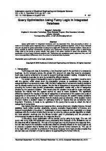
2 MOTIVATION We will motivate our case with an illustrative example. Consider the conceptual schema of the data warehouse of some retail store chain as depicted in figure 1. By adopting a multidimensional terminology, there are three dimensions, Product, Location and Time with several category attributes. The arrows define functional dependencies in database terms. Each path from a terminal attribute, e.g. Article, to the Top category in the respective dimension defines a classification hierarchy (figure 1). Parallel paths result in parallel hierar-
Related Work
Product
3
Time
Top
Top
Top
Branch
Year
Country
Group
Quarter
Family
Publisher
Tax
Month
Price
Article
Day
6)
Location
State
Manager
City
Budget
Shop
Qty
Figure 1: Sample conceptual schema of a retail store chain chies. For the OLAP user these paths describe the basic navigation constructs for drill-down and roll-up operations. In the sample database there are four measures. Only the quantity sold (Qty) is given per article, day and shop. The other measures are gathered at a higher granularity. For example the retail chain has the policy that the prices are the same in all of its shops and they change only quarterly. The budget is assigned once a year to each shop. Taxes are depending on the state the shop is located in and may also change quarterly. In a relational database this schema is mapped to a snowflake schema with a fact table for each measure and one dimension table for each category attribute with according foreign key relationships [18]. To prevent lots of joins in the examples we will assume a star schema with one denormalized table for each dimension (figure 2 left side). Consider the following query: “Give me the turnover per branch, region and quarter for the sales in Germany in 1999.” The appropriate SQL query is printed on the right side of figure 2. In figure 3 there are two query plans for this query. To emphasize the important matters the dimension tables and the respective joins have been removed. Both query plans are yielding the same result. The plan in figure 3a is straight-forward and similar to the one chosen by any relational DBMS (before optimization). The plan in figure 3b makes only sense if the gray areas are materialized views. In order to determine that the query is also derivable from the views, the optimizer must be aware of the facts that 0
1) the applied aggregation function in view 1 and view 2 is SUM and SUM is additive, 2) the granularity, i.e. the aggregation level, of view 2 is finer than the requested one and thus it can and must be further aggregated, 3) the union of the regions “G-North” and “G-South” yields whole “Germany”, 4) Turnover can generally be computed as Turnover = Qty • Price, 5) the already summarized value of Qty in view 2 can still be used to compute the Turnover at higher granularities, Fact_Qty Fact_Price Fact_Budget Fact_Tax Product Location Time
(Article, Shop, Day, Qty) (Article, Quarter, Price) (Shop, Year, Budget) (State, Quarter, Tax) (Article, Family, Group, Branch, Publisher) (Shop, City, State, Country, Manager) (Day, Month, Quarter, Year)
Price,
although given at granularity (Article, Quarter), can be used at any finer granularity as well, because prices for a given product and quarter are the same for all months, days, shops. If now the views 1, 2, and 3 were materialized views, either manually created or cached results from previous queries, this plan might actually be cheaper than the original one. In this case only the compensations, i.e. the operations outside of the gray boxes, would have to be executed and because of the high aggregation levels of the views these are likely to be much smaller than the original fact tables.
3 RELATED WORK The question of derivability has been investigated for some time. First concepts were examined for statistical and scientific database systems. Nowadays the topic has gained importance once more as possible optimization strategy for large data warehouse systems. A short classification of related work is given below.
Preconditions for Derivability An important query optimization technique is algebraic transformation of queries. [27] suggest how to speed up the computation of a relational SPJ query by generating several execution plans considering different choices of access paths to base relations and different join sequences. [33] and [7] extend this idea to queries involving aggregate functions and grouping by using push-down and pullup techniques. [8] in addition to its predecessor also consider aggregate functions. Although algebraic transformations are a necessary prerequisite for query rewriting, these approaches do not utilize materialized views. They also do not exploit the multidimensional semantics with dimensional hierarchies.
First Definitions of Derivability [28] introduces the notion of derivability in the context of statistical database systems and divides summary data into different classifications. One classification may be derivable from another one by inference rules. [12] exploits algebraic transformation of query graphs to detect common subexpressions between queries. If a new query contains at least part of an already evaluated one, this part can be replaced. This is the beginning of utilizing materialized views. The method is extended in several articles, e.g. [6], [32], [24], [10] or [11]. The algorithms published in these papers most of the time treat special cases that are of little relevance for data warehouses. Furthermore many of the algorithms are of exponential complexity. Our approach reduces complexity dramatically as we exploit additional information and focus on a set of typical queries in the area of OLAP.
Semantic Query Optimization and Derivability Semantic query optimization modifies queries due to the knowledge of the contents of the database and the application area of the data which are stored in the database. For that the techniques used SELECT FROM WHERE
GROUP BY
P.Branch, L.Region, T.Quarter, SUM(Qty*Price) AS Turnover Fact_Qty FQ, Fact_Price FP, Product P, Location L, Time T FQ.Article = P.Article AND FQ.Shop = L.Shop AND FQ.Day = T.Day AND FP.Article = P.Article AND FP.Quarter = T.Quarter AND L.Country = ‘Germany’ AND T.Year = ‘1999’ P.Branch, L.Region, T.Quarter
Figure 2: Tables of the scenario and SQL query
4
Aggregate Views ∪ Σ P.Branch
σ T.Year=1999
Σ P.Branch
Σ P.Branch
L.Region T.Quarter
L.Region T.Quarter
L.Region T.Quarter
π
σ L.Country=”G-North”
σ L.Country=”Germany” AND T.Year=199
π
Qty • Price = Turnover
π
Qty • Price = Turnover
Σ P.Article Qty*Price = Turnover
L.City T.Month
σ L.Region=”G-South” AND
σ L.Country=”Germany”
T.Year=1999
Fact_Qty
Fact_Qty
Fact_Price
Fact_Price
Fact_Qty
View V1
a) Plan based on raw data
Fact_Price
View V2
View V3
b) Rewritten plan based on materialized views
Figure 3: Possible query plans for the sample query. in this area try to detect rules and dependencies among the current values ([34], [15]). These rules then can be used for derivability. Another important paper about derivability using aggregated views is [30] . Here the combination of multiple query fragments is introduced. The main difference between our approach to semantic query optimization and previous methods is that we do not need (and do not use) any knowledge about the contents of the database except for dimensions and hierarchies and information about the measures to derive a query from a computed result while they primarily have to generate the rules for the complete raw date before applying these rules for derivability. This is also the reason why this kind of semantic query optimization is not feasible in the context of data warehouses.
completely describe these simple aggregate queries by using only the components printed in italics above. However, it is necessary to make two further assumptions:
Semantics in combination with summarizability is studied in [22]. Here three conditions for summarizability are introduced. Of special importance for this article are the different aggregation types of measures (flow, stock and value-per-unit).
Since the class of queries we describe has multidimensional characteristics and in fact all conditions for derivability given in the following can also be applied in multidimensional OLAP systems, we will use a multidimensional terminology. The goal of the following section is to express the additional semantics of dimension hierarchies and measures.
Derivability using Aggregation Lattices The aggregation lattice ([14], [4], [13]) forms the basis for derivability in the multidimensional context. According to the aggregation level, aggregates can be arranged in a lattice structure which reflects the derivability relation. However, these approaches do not consider any kind of restrictions. All related work has in common, that the semantics of composite measures is not considered.
4 AGGREGATE VIEWS Since the problem of query derivability in general is NP-hard [31], the focus of this article is not to investigate all possibilities of the derivability of relational queries. Instead, we restrict the scope of interest to the typical class of data warehouse queries: star (or snowflake) queries with aggregations and restrictions on measures possibly computed like Turnover in section 2. Thus, a template for the aggregate queries we want to consider is the following: SELECT FROM WHERE GROUP BY
, , AND
Clearly the query in section 2, as well as most other data warehouse queries, belongs to this category. For the formalization of sufficient conditions for derivability we introduce a compact formalism to
0
1) Measures are uniquely identified by their names. This does not actually restrict the class of possible queries but simplifies their description. 2) All joins are lossless. Otherwise the join might eliminate tuples unnoticedly and it would not be possible to determine derivability. All tuples which are not desired in the result set must explicitly be removed by the WHERE clause. Note, that lossless joins are the default in data warehouse queries.
4.1. Dimensions A dimension provides semantic information about the hierarchical relationships between its elements which are classified for example into product groups or geographic regions. This information is heavily used in queries on the one hand to define the aggregation level, i.e. the granularity, and on the other hand to restrict the scope of interest. Both can be exploited for query rewriting. Definition 1: A dimension schema consists of a partially ordered set of category attributes (D ∪ {TopD};→) where D = {D1,...,Dn} and “→” denotes the functional dependency relation. TopD is the special level which is maximal with respect to “→”, i.e. Di→− TopD for each Di∈ D. The instances c ∈dom(Di) of a category attribute Di ∈D are called categories of Di. Moreover, dom(TopD) := {‘ALL’}. The instance of a dimension D is the set of all category attributes. Dimension schemas were already illustrated in figure 1. Each path to Top in a dimension schema specifies a hierarchy as the one shown in figure 4. By defining dom(Top):={‘ALL’} it is guaranteed that all classification hierarchies are trees having “ALL” as the single root node, a property that is necessary in the context of summarizability [21]. In this article we consider dimensions only as unordered sets of elements.
Aggregate Views
Top
4.2
Branch
Family
Brown Goods Video
Audio
Product
...
White Goods
Computers ...
Group
Location
ALL
Products
HomeVCR
Camcorder Time
Article
Qty
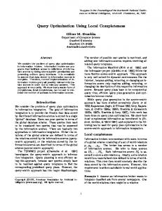
Figure 5: Multidimensional view of the quantity fact table
Figure 4: Sample product hierarchy
4.2. Simple Aggregate Views and Queries Using the definition of a dimension it is possible to define a data structure for simple aggregate queries or views by assuming that all joins are determined implicitly by foreign keys to the respective tables. In the context of this work the difference between a query and a view is of no interest. Thus we will use the same notation for an aggregate view and an aggregate query. Definition 2: A simple aggregate view (or query) is a structure 1 V = [G, M, S] where • G = (G1,...,Gn) is the granularity consisting of a set of category attributes2 which are functionally independent, i.e. for each Gi, Gj ∈ G: Gi → / Gj, • M = (AGG1(M1),..., AGGm(Mm)) is a set of aggregated measures where AGGi ∈ {NONE, SUM, COUNT, MIN, MAX} denotes the applied aggregation operation, • S is a logical predicate defining the scope restriction. In the definition of a simple view the SQL aggregation operation AVG is missing. This is because the AVG is not additive in the sense of [6], i.e. averages are not derivable from averages. However, if derivability is concerned an AVG operation can be internally mapped to SUM and COUNT. The operation NONE means that no aggregation was performed. We call a simple aggregate view a raw data view for measure Mi if NONE(Mi) ∈M. The raw granularity of a measure, denoted as Gran(M), is the granularity of its raw data view. In the multidimensional perspective an aggregate view can be illustrated as a data cube (figure 5). Therefore, we will refer to the contents of the cube as data cells. Since aggregate views define queries on the raw data, the scope can be an arbitrary logical expression involving any dimension attibutes functionally dependent on some granularity attribute in the respective raw data view for one of the measures. Example 1: A raw data view for the quantity fact table in section 2 is VQty = [(P.Article, L.Shop, T.Day), NONE(Qty), ∅]. As in this example we will use dimension aliases as prefixes for the category attributes to make the context clear. For simplicity we will not specify empty scopes or aggregate restrictions. Thus we might just write VQty = [(P.Article, L.Shop, T.Day), NONE(Qty)] for the view above. Similar definitions exist for VPrice, VBudget and VTax. 1. The definition of G and M as tuples is for the sake of simplicity only; as in the relational data model the order of the attributes does, at least from the conceptual point of view, not matter. Therefore, we will also apply the set operators like ∈, ∪, ∩, = to G and M. 2. Category attributes are used to describe the granularity, i.e. the aggregation level. Thus each Gi = Dj in some dimension.
The simple aggregate view V2 in figure 3 could be specified as V2 = [(P.Article, L.City, T.Month), SUM(Sales), (L.Region=”G-South” ∧ T.Year=”1999”)]. To specify the turnover we need a notation for composite measures which will be introduced in section 4.6.
4.3. Operations on Simple Aggregate Views This section informally introduces our notation for operations on simple aggregate views, because the definition of the operators should be intuitively clear. The projection πE(M) is used to project a subset of the measures or an expression thereof with the operators {+, -, •, /, cmin, cmax}. The operations cmin and cmax are not part of SQL, but nonetheless common in data warehouse applications. They are used to find the smaller (respectively larger) value of two measures (cell minimum/ maximum, e.g. cmin(Qty_Sold, Qty_Stock)) in contrast to the MIN and MAX aggregation operations which find the minimum and maximum of one measure for a certain group of cells. The scope restriction σS’ is used to apply further restrictions to the view. It is defined only, if the predicate S’ contains only dimension attributes functionally dependent on some Gi ∈ G. In this case σS’([G, M, S]) = [G, M, S∧S’]. Most important are aggregations. An aggregation groups cells at a finer granularity into cells at a coarser granularity and applies an aggregation operation on the measures. The finer/coarser relationship can be visualized by a lattice structure as suggested in [14]. Definition 3:
A granularity, i.e. a set of category attributes
G’ = (G1’,...,Gk’) is coarser (or equal) than a granularity G = (G1,...,Gn), denoted as G’ ≥ G, if and only if for each Gj' ∈G’ there is a Gi ∈G such that Gi→Gj’. In this case G is said to be finer than G’, i.e. G ≤ G’. The aggregation of a simple aggregate view V = [G, (AGG1(M1), ... AGGm(Mm)), S] by a family of aggregate functions A = (AGG1’, ..., AGGm’) to the granularity G’, denoted as A(G’, V) is well-defined if G’ ≥ G and AGGi’ = AGGi or AGGi = NONE. In this case A(G’, V) = [G’, (AGG1’(M1), ... AGGm’(Mm)), S].
The term well-defined in the last definition means that the result again can be described as simple aggregate view. In general the introduced operations are not as powerful as the relational algebra because not all relational algebra expressions can be defined in terms of these. This is by intention, because the goal is only to give sufficient conditions for certain special cases of queries.
4.4. Joins of Aggregate Views Often queries request several measures possibly contained in multiple data cubes or multiple fact tables in a star schema. Such queries are also the basis for the computation of composite measures. Consider the query: “Give me the quantities sold and on stock for each product and day”. If these two measures were stored in diffe-
4.5
Multiplexable Measures and Aggregation Types
rent fact tables of a star schema an inner join would not show tuples for products sold but out of stock. Thus, as stated in the second requirement in section 4 we assume a lossless join semantic which requires an outer join. Definition 4: The join of two simple aggregate views V1 = [G1, M1, S1] and V2 = [G2, M2, S2], denoted as V1 V2, is well-defined, if it is lossless and G1 = G2. In this case the result is a simple aggregate query V1 V2 = [G1, M1 ∪ M2, S1 ∧ S2].
4.5. Multiplexable Measures and Aggregation Types The join defined in the previous section is meant as an equi-join on all granularity attributes. However, the condition that the granularities must be the same would forbid the following query: “Give me the turnover as the product of the quantities sold and the respective price for each article and day.” These measures are given at different granularities. In the sample schema Gran(Price) = (P.Article, T.Quarter). This does not mean that the price for a product cannot be determined for each day and shop, but that it is the same for each day and shop in a given quarter, and even for each customer and whatever other dimension there may be in the database. Thus, it is possible to use the price at a finer granularity as its raw granularity, e.g. (P.Article, T.Day, L.Shop). Measures of this kind are called multiplexable and are introduced by [2]. Therefore, we present here only a short overview and refer for a more in detail discussion to the original article. Definition 5: A measure M is multiplexable if for all granularities finer than its raw data granularity Gran(M) the values can be disaggregated by the identity function. The fact that prices are multiplexable is related to the aggregation type of a measure which is introduced in [22], tells something about summarizability and can be FLOW (e.g. turnover, sold quantity), STOCK (e.g. inventories) or VPU (value-per-unit; e.g. prices) in general. Accordingly to [2] we restrict ourselves to the aggregation type Type(M) ∈{FLOW, VPU} for a measure M. Axiom 1: A measure is multiplexable if and only if it is of the aggregation type VPU. Definition 6: The multiplex operator MUX for the granularity G’ applied to a raw data view V = [G, (NONE(M1), ..., NONE(Mm)), S], denoted as MUX(G’, V) = [G’, MUX(M1), ..., MUX(Mm), S], is welldefined if G’ ≤ G and Type(Mi) = VPU for each i = 1, ..., m.
For aggregations (definition 3) a measure MUX(M) can be assumed as not aggregated. For each cell c” at a granulariy G” with G’ ≤ G” ≤ G the value of any cell at G’ which belongs to the group of c” can be chosen, because all share the same value of the corresponding original cell at granularity G (see figure 6 for an illustration). This is also the motivation for the term “multiplexable” because one value at the coarser granularity is multiplexed to many cells at the finer granularity.
Germany G=L.Country
G’=L.State
FLOW op FLOW
FLOW
FLOW op VPU VPU op FLOW VPU op VPU
7
7
7
7
L.Region and L.State.
4.6. Composite Measures As already pointed out, measures are often derived from other measures by simple formulas or business rules. Frequent examples are Turnover = Qty • Price or TurnoverTax = Turnover • Tax. We call these measures composite. The conceptual granularity of such a measure is that of the finest of the operands in its definition. For example Turnover has the same granularity as Qty. This is because for the computation a join of VQty and VPrice is necessary. If formulas are specified on a conceptual level, aggregate views of the operands of the formula can be used to derive the result (section ). Definition 7: A formula M = M1 op M2, where op ∈ {+, -,•, /, cmin, cmax}, is well-defined if the join between the respective raw data views of M1 and M2 is well-defined and the aggregation type of M can be determined by table 1. Then the granularity of M is determined as Gran(M) = min(Gran(M1), Gran(M2)). Of course the operands M1 and M2 can be composite measures themselves, like TurnoverTax = Turnover• Tax. Although in the following we will only consider non-nested definitions of composite measures, the laws of distributivity and associativity can be used to derive much more rewriting possibilities for queries in the general case.
5 DERIVABILITY OF SIMPLE AGGREGATE VIEWS Derivability of multidimensional aggregates is the condition that has to be fulfilled to compute the result of an aggregate query based on the values of one or more aggregate views. Informally a query Q defined on a set of tables is derivable from a set of views V, if it can be computed alone by using these views instead of the original tables. In other words, there must exist a rewriting for Q. More formally derivability can be defined as follows: Definition 8: An aggregate query Q is derivable from a set of aggregate views V = {V1, ..., Vv} if and only if a rewriting of Q involving only the views in V exists.
*
/
cmin
cmax
VPU
FLOW
FLOW
FLOW
FLOW
VPU
VPU
VPU
7
Figure 6: Multiplexing of a value-per-unit measure which is defined at granularity L.Country to
FLOW VPU
G-North
7
BY BW BRB NRW
op
+-
G-South G”=L.Region
Table 1: Resulting aggregation types for composite measures. Empty fields signal that the formula is not well-defined. Aggregation Types of the Operands
7
VPU
Derivability of Simple Aggregate Views
5
45 60
45 60
SUM(M1•M2)
29 26
29 26
SUM(M1+M2)
SUM(M1)+SUM(M2)
13 14 16 12
V1
M1•M2
V
15,14 12,14
7,3 8,3
M1+M2
7,6 8,8
V1
9,5 3,9
SUM(M1)•M2
21 45 24 15
9,5 3,5
15,3
V2
15 12
14 14
SUM(M1)
SUM(M2)
3 3
V2
5 5
12,5
15 12 SUM(M1)
MUX(M2)
7 8
9 3
6 8
VR1
5 9 VR2
7 8 VR1
9 3
6 8
5 9
7 8
VR2
VR1
Figure 7: Deriving a sum from sum values The definition of a simple aggregate query Q implicitly involves the respective raw data views. In fact, a reformulation of Q using only raw data is the trivial rewriting that always exists. If the query can be derived from a single aggregate view several well known conditions like the compatibilities of the granularities or the aggregation operators have to be compared ([3]). In [2] the conditions are extended for granularities after involving the the multiplex operator. This article extends the considerations regarding to the derivability of composite measures, which is presented in the next paragraph.
Special Cases of Derivability for Composite Measures An interesting topic about derivability is the possibility of deriving aggregate queries involving composite measures not only from views containing exactly the same measure, but also from aggregate views containing aggregations of the corresponding raw measures. Theorem 1: Let Q = [GQ, AGGQ(MQ), SQ] be an aggregated query where MQ = M1 op M2 is a composite measure. Let V1 = [G1, AGG1(M1), S1] and V2 = [G2, AGG2(M2), S2] be aggregated views and let VR1[GR1, NONE(M1)] and VR2[GR2, NONE(M2)] be the respective raw data views. Then Q is derivable from V1 and V2 if • G1 ≤ GQ, • the scope restriction SQ implies SVi and σSQ(Vi) is welldefined for i = 1, 2 and • G2 ≤ GQ and one of the cases 1, 2 or 3 in table 2 applies or • G1 ≤ GQ, • the scope restriction SQ implies SVi and σSQ(Vi) is welldefined for i = 1, 2 and • V2 is a raw data view, i.e. V2 = VR2, and GQ ≤ G2 and one of the cases 4 or 5 in table 2 applies.
9 3
3
5
7 8
VR2
9 3 VR1
3
5 VR2
Figure 8: Deriving a product from sum values In the first case let GV = max(G1, G2). Then a rewriting is
AGGQ(GQ, π(MQ = M1 op M2) (σS (AGGQ(GV, V1)
AGGQ(GV, V2)))
In the second case let GV = min(GQ, G2). Then a rewriting is AGGQ(GQ, π(MQ = M1 op M2) (σS (AGGQ(GV, V1) MUX(GV, V2))). If one considers the views as subqueries, a group-by push-down or eager aggregation similar to the methods proposed in [33] or [7] is applied. In general these methods would not work here, because first the information that MQ = M1 op M2 is necessary, and second, the aggregation type of the measure must be known for the cases 4 and 5. However, the proposed rewriting technique can be seen as a semantic extension of this work. As explained in section 4.5 each measure M has an aggregation type Type(M) which is either FLOW or VPU. For the first three cases equivalence holds because of the laws of associativity and distributivity for summation and min/max operations. Figure 7 illustrates the theorem for case 3 in the context of simple aggregate queries. Assume two two-dimensional raw data views VR1 = [G1, NONE(M1)] and VR2 = [G2, NONE(M2)] and the aggregate query Q = [GQ, SUM(MQ)] where MQ = M1 + M2. The operator graph in the left part of the figure shows the usual way of processing this query. First VR1 and VR2 are joined, then the measures are added in each cell (or tuple) and finally the aggregation is performed. The view V = [Gv, SUM(MQ)] with GV ≤ GQ could be used to derive Q. However, as illustrated on the right side, it is possible to aggregate first and then perform the join and add the measures. If the views V1[Gv1, SUM(M1)] and V2[Gv2, SUM(M2)] were materialized, the query could be derived from V1 and V2 as well. For the remaining combinations of aggregation operations and operators on the measures counter examples can be found, but are not presented here due to the lack of space.
Table 2: Derivability of composite measures No.
AGGQ( M1 op M2 )= AGG1(M1) op’ AGG2(M2)
Type(M1)
Type(M2)
1
MIN( cmin(M1, M2) )= cmin( MIN(M1), MIN(M2) )
FLOW, VPU
FLOW, VPU
2
MAX( cmax(M1, M2) )= cmax( MAX(M1), MAX(M2) )
FLOW, VPU
FLOW, VPU
3
SUM( M1 ± M2 )= SUM(M1) ± SUM(M2)
FLOW, VPU
FLOW, VPU
4
SUM( M1 • M2 )= SUM(M1) • MUX(M2)
FLOW,
VPU
5
SUM( M1 / M2 )= SUM(M1) / MUX(M2)
FLOW,
VPU
6
Future Work
Most interesting are cases 4 and 5. Since multiplication is commutative, there also exists a symmetric case for case 4. The reason is similar for the division of a measure by a value-per-unit measure, although there is no symmetric equivalent. For illustration we will use case 4. Basically what is stated here is that SUM(M1• M2) = SUM(M1)• M2! Intuitively this is clear if M2 is a constant. And in fact this is the reason why it works here. Consider the example in figure 8 with the raw data views VR1 = [GR1, NONE(M1)] and VR2 = [GR2, NONE(M2)] and the aggregate query Q = [GQ, SUM(MQ)] where MQ = M1 • M2 and Type(M2)=VPU. To make it clear, assume the formula Turnover = Qty • Price. The left part of the figure shows the simple execution, first computing the turnover at raw data level and then aggregating. Obviously already computed turnover values, if for example the view V1 was materialized, could be used as well to derive the query. But the key point here is that also aggregated quantities as in V2 can be used in combination with VR2 to derive the result. This means that the group-by operation can be pushed down over the join because M2 is of type value-per-unit. Note that this makes query processing faster even if the view V2 was not materialized. In fact any aggregate query Q = [GQ, SUM(MQ)] can be computed by first aggregating VR1 to the granularity G2 and then performing the join. Also, any materialized view like V2 can be used to derive Q as long as GV2 ≤ G2. In the example GV2 = G2, otherwise the MUX operator must be applied to adjust the granularity. In any case the values in a cell of VR2 are constant for all cells in VR1 or any view like V2 which belong to the same group as this cell after the join.
7 SUMMARY
After investigating the operations MIN, MAX and SUM the special case of the COUNT remains. Because it only counts elements, it does not depend on the operator. However, it does depend on the semantics of the join (inner/outer) and the default treatment of NULL values. [18] states therefore that the common SQL COUNT operation is problematic in data warehouse queries. There are special cases where the counting of one of the operand measures yields the same result as counting the composite measure, but additional constraints must be satisfied. For example if Price is defined for every product and each quarter where the product was sold, the count of Turnover is the same as the count of Qty.
The utilization of materialized views has gained much attention, especially as an optimization strategy for aggregate queries in data warehouses. A necessary prerequisite in order to compute a query from one or more aggregate views is that there exists a rewriting for the query based on the views instead of the raw data. In this article we identify several cases where rewritings exist. All conditions make use of additional semantics which in general is not available at a purely relational level. However, the provided rewritings in these cases are simple and still of great practical interest.
REFERENCES 1
Albrecht, J.; Bauer, A.; Deyerling, O.; Günzel, H.; Hümmer, W.; Lehner, W.; Schlesinger, L.: Management of multidimensional Aggregates for efficient Online Analytical Processing, in: International Database Engineering and Applications Symposium (IDEAS’99, Montreal, Canada, August 1-3), 1999
2
Albrecht, J.; Hümmer, W.; Lehner, W.; Schlesinger, L.: Using Semantics for Query Derivability in Data Warehouse Applications, appears in: Proceedings of the 4th International Conference on Flexible Query Answering Systems (FQAS’00, Warsaw, Poland, October 25 - 25), 2000
3
Albrecht, J.; Günzel, H.; Lehner, W.: Set-Derivability of Multidimensional Aggregates, in: Proceedings of the First International Conference on Data Warehousing and Knowledge Discovery (DAWAK’99, Florence, Italy, August 30 - September 1), 1999
4
Baralis, E.; Paraboschi, S.; Teniente, E.: Materialized Views Selection in a Multidimensional Database, in: 23rd International Conference on Very Large Data Bases (VLDB’97, Athen, Griechenland), 1997, S. 156-165
5
Cabibbo, L.; Torlone, R.: From a Procedural to a Visual Query Language for OLAP, in: Proceedings of the 10th International Conference on Scientific and Statistical Data Management (SSDBM’98, Capri, Italy, July 1-3), 1998
6
Chen, M. C.; McNamee, L.; Melkanoff, M.: A Model of Summary Data and its Applications in Statistical Databases, in: Proceedings of the 4th International Working Conference on Statistical and Scientific Database Management (SSDBM’88, Rome, Italy, June 21-23), 1988
7
Chaudhuri, S.; Shim, K.: Optimizing Complex Queries: A Unifying Approach, Technical Memo HPL-DTD-95-20, Hewlett Packard Laboratories, Palo Alto, California, 1995
8
Chaudhuri, S.; Shim, K.: Optimizing Queries with Aggregate Views, in: 5th International Conference on Extending Database Technology (EDBT’96, Avignon, Frankreich, 25.29. März, 1996)
9
Codd, E.F.: Derivability, Redundancy and Consistency of Relations Stored in Large Data Banks, in: IBM Research Report RJ 599, San Jose, California, 1969
6 FUTURE WORK Our future goal is to extend 3 5 3 5 the set of semantic conditions for the derivability MIN(M2) < 6 especially of those queries V2 which are restricted by the MIN(M1) < 6 3 5 6 HAVING-clause. The MIN(M2) < 7 present paper does not deal with this problem because of 7 9 9 8 7 9 9 8 the concentration on the 8 3 5 6 8 3 5 6 derivability of composite V VR2 R1 measures. To illustrate the general idea of our future Figure 9: Deriving a HAVINGwork we refer to figure 9. It restricted table from a HAVINGshows the possibility of restricted table for min values deriving a query with the aggregation operator MIN from another query with the same aggregation operator, but with different restrictions after the aggregation. We will investigate this derivability problem for the standard aggregation functions and the common comparison operators. Another future topic is to integrate the semantic conditions into the prototypical ROLAP server CUBESTAR. A subset of the cases presented here has already been successfully tested in [1].
10 Cohen, S.; Nutt, W.; Serebrenik, A.: Rewriting Aggregate Queries Using Views, in: 18th Symposium on Principles of Database Systems (PODS’99, Philadelphia, Pennsylvania, USA, May 31 - June 2), 1999
Summary 11 Cohen, S.; Nutt, W.; Serebrenik, A.: Algorithms for Rewriting Aggregate Queries Using Views, in: Proceedings of the International Workshop on Design and Management of Data Warehouses (DMDW’99, Heidelberg, Germany, June 14 - 15), 1999 12 Finkelstein, S.: Common Expression Analysis in Database Applications, in: Proceedings of the International Conference on the Management of Data (SIGMOD’82, Orlando, Florida, June 2-4), 1982 13 Gupta, H.; Harinarayan, V.; Rajaraman, A.; Ullman, J.D.: Index Selection for OLAP, in: Gray, A.; Larson, P.-A.: 13th International Conference on Data Engineering (ICDE’97, Birmingham, Großbritannien, April 7-11), 1997 14 Harinarayan, V.; Rajaraman, A.; Ullman, J.D.: Implementing Data Cubes Efficiently, in: 25th International Conference on Management of Data, (SIGMOD96, Montreal, Quebec, Canada, June 4-6), 1996 15 Han, J.; Huang, Y.; Cercone, N.; Fu, Y.: Intelligent Query Answering by Knowledge Discovery Techniques, in: IEEE Transactions on Knowledge and Data Engineering (TKDE) 8(1996)3, S. 373-390 16 Hopcroft, J.E.; Ullman, J.D.: Introduction to Automata Theory, Languages, and Computation, Reading; Massachusetts, Addison-Wesley, 1979 17 N.N.: IBM DB2 Universal Database Administration Guide, Version 6, IBM, 1999 18 Kimball, R.: The Data Warehouse Toolkit, second edition, New York, Chichester, Brisbane, Toronto, Singapur: John Wiley & Sons, Inc., 1996 19 Larson, P.- A.;Yang, H.Z.: Computing Queries from Derived Relations, in: Proceedings of the 11th International Conference on Very Large Data Bases (VLDB’85, Stockholm, Schweden, August 21-23), 1985 20 Lehner, W.: Modeling Large Scale OLAP Scenarios, to appear in: 6th International Conference on Extending Database Technology (EDBT’98, Valencia, Spain, March 23-27), 1998
7 23 Levy, A.Y.; Mendelzon, A.O.; Sagiv, Y.; Srivastava, D.: Answering Queries Using Views (Extended Abstract), in: Proceedings of the 14th Symposium on Principles of Database Systems (PODS '95, San Jose, Ca., USA, May 22-25), 1995 24 Nutt, W.; Sagiv, Y.; Shurin, S.: Deciding Equivalence among Aggregate Queries, in: 17th Symposium on Principles of Database Systems (PODS’98, Seattle, Washington, USA, June 1-3), 1998 25 N.N.: Oracle8i Tuning, Systems Manual, Oracle Corporation, 1999 27 Selinger, P.G.; Astrahan, M.M.; Chamberlain, D.D.; Lorie, R.A.; Price, T.G.: Access Path Selection in a Relational Database Management System, in: Bernstein, P.A. (Hrsg.): Proceedings of the 1979 ACM International Conference on Management of Data (SIGMOD’79, Boston, Massachusetts, Mai 30 - June 1), 1979 28 Sato, H.: Handling Summary Information in a Database: Derivability, in: Proceedings of the 1981 ACM International Conference on Management of Data (SIGMOD’81, Ann Arbor, Michigan, USA, April 29-May 1), 1981 29 Shim J.; Scheuermann, P.; Vingralek, R.: Dynamic Caching of Query Results for Decision Support Systems, in: Proceedings of the 11th International Conference on Scientific and Statistical Database Management (SSDBM’99, Cleveland, Ohio, USA, July 28-30) 30 Srivastava, D.; Dar, S.; Jagadish, H.V.; Levy, A.Y.: Answering Queries with Aggregation Using Views, in: Proceedings of 22th International Conference on Very Large Data Bases (VLDB’96, Mumbai (Bombay), India, September 3-6), 1996 31 Sun, X.-H.; Kamel, N.; Ni, M.N.: Solving Implication Problems in Database Applications, in: Proceedings of the 1989 ACM SIGMOD International Conference on Management of Data (SIGMOD’89, Portland, Oregon, USA, May 31 - June 2), 1989 32 Ullman, J.D.: Principles of Database and Knowledge-Base Systems, Volumes I and II, Computer Science Press, Rockville, 1988/89
21 Lehner, W.; Albrecht, J.; Wedekind, H.: Normal Forms for Multidimensional Databases, in: Proceedings of the 10th International Conference on Scientific and Statistical Data Management (SSDBM’98, Capri, Italy, July 1-3), 1998
33 Yan, W.P.; Larson, P.A.: Eager Aggregation and Lazy Aggregation, in: Dayal, U.; Gray, P.M.D.; Nishio, S. (Hrsg.): Proceedings of the 21st International Conference on Very Large Data Bases (VLDB’95, Zürich, Switzerland, September 11-15), 1995
22 Lenz, H; Shoshani, A.: Summarizability in OLAP and Statistical Databases, in: 9th International Conferenc on Statistical and Scientfic Databases, (SSDB’97, Olympia, Washington, August 11-13), 1997
34 Yu, C.T.; Sun, W.: Automatic Knowledge Acquisition and Maintenance for Semantic Query Optimization, in: IEEE Transactions on Knowledge and Data Engineering (TKDE) 1(1989)3