Query Processing and Optimization in Modern Database ... - mediaTUM

¨ M UNCHEN ¨ T ECHNISCHE U NIVERSIT AT Fakultät für Informatik Lehrstuhl III – Datenbanksysteme

Query Processing and Optimization in Modern Database Systems Viktor Leis

Vollständiger Abdruck der von der Fakultät für Informatik der Technischen Universität München zur Erlangung des akademischen Grades eines Doktors der Naturwissenschaften (Dr. rer. nat.) genehmigten Dissertation.

Vorsitzender: Univ.-Prof. Dr. Hans-Joachim Bungartz Prüfer der Dissertation: Univ.-Prof. Dr. Thomas Neumann, Prof. Michael Stonebraker, Ph.D. (MIT, Cambridge, USA) Univ.-Prof. Alfons Kemper, Ph.D.

Die Dissertation wurde am 25.05.2016 bei der Technischen Universität München eingereicht und durch die Fakultät für Informatik am 30.09.2016 angenommen.

Abstract Relational database management systems, which were designed decades ago, are still the dominant data processing platform. Large DRAM capacities and servers with many cores have fundamentally changed the hardware landscape. Traditional database systems were designed with very different hardware in mind and cannot exploit modern hardware effectively. This thesis focuses on the challenges posed by modern hardware for transaction processing, query processing, and query optimization. We present a concurrent transaction processing system based on hardware transactional memory and show how to synchronize data structures efficiently. We further design a parallel query engine for many-core CPUs that supports the important relational operators including join, aggregation, window functions, etc. Finally, we dissect the query optimization process in the main memory setting and show the contribution of each query optimizer component to the overall query performance.

iii

Zusammenfassung Relationale Datenbankmanagementsysteme, deren ursprüngliche Entwicklung bereits Jahrzehnte zurückliegt, sind auch heute noch die dominierende Datenverarbeitungsplattform. Rechner mit großen DRAM-Kapazitäten und vielen Kernen haben die Hardwarelandschaft jedoch fundamental verändert. Traditionelle Datenbanksysteme wurden für Systeme entwickelt, die sich sehr von aktuellen unterscheiden, und können deshalb moderne Hardware nicht effektiv nutzen. Die vorliegende Arbeit befasst sich mit den Herausforderungen moderner Hardware für die Transaktionsverarbeitung, Anfrageverarbeitung und Anfrageoptimierung. Zunächst präsentieren wir ein Transaktionsverarbeitungssystem basierend auf Hardware Transactional Memory und zeigen wie Datenstrukturen effizient synchronisiert werden können. Darüber hinaus entwickeln wir eine parallele Anfrageverarbeitungkomponente für Rechner mit vielen Kernen, welche unter anderem die wichtigen relationalen Operatoren Verbund, Aggregation und Windowfunktionen unterstützt. Schließlich untersuchen wir den Anfrageoptimierungsprozess in Haupspeicherdatenbanken und zeigen den Beitrag der einzelnen Optimererkomponenten zu der Gesamtanfragegeschwindigkeit.

v

Contents List of Figures

xiii

List of Tables

xvii

1

2

Introduction 1.1 Column Stores . . . . . . . . . . . . 1.2 Main-Memory Database Systems . . . 1.3 The Challenges of Modern Hardware . 1.4 Outline . . . . . . . . . . . . . . . .

. . . .

. . . .

. . . .

. . . .

. . . .

. . . .

. . . .

. . . .

. . . .

. . . .

. . . .

. . . .

. . . .

. . . .

. . . .

. . . .

. . . .

Exploiting Hardware Transactional Memory in Main-Memory Databases 2.1 Introduction . . . . . . . . . . . . . . . . . . . . . . . . . . . . . . . 2.2 Background and Motivation . . . . . . . . . . . . . . . . . . . . . . 2.3 Transactional Memory . . . . . . . . . . . . . . . . . . . . . . . . . 2.3.1 Hardware Support for Transactional Memory . . . . . . . . . 2.3.2 Caches and Cache Coherency . . . . . . . . . . . . . . . . . 2.4 Synchronization on Many-Core CPUs . . . . . . . . . . . . . . . . . 2.4.1 The Perils of Latching . . . . . . . . . . . . . . . . . . . . . 2.4.2 Latch-Free Data Structures . . . . . . . . . . . . . . . . . . . 2.4.3 Hardware Transactional Memory on Many-Core Systems . . . 2.4.4 Discussion . . . . . . . . . . . . . . . . . . . . . . . . . . . 2.5 HTM-Supported Transaction Management . . . . . . . . . . . . . . . 2.5.1 Mapping Database Transactions to HTM Transactions . . . . 2.5.2 Conflict Detection and Resolution . . . . . . . . . . . . . . . 2.5.3 Optimizations . . . . . . . . . . . . . . . . . . . . . . . . . . 2.6 HTM-Friendly Data Storage . . . . . . . . . . . . . . . . . . . . . . 2.6.1 Data Storage with Zone Segmentation . . . . . . . . . . . . . 2.6.2 Index Structures . . . . . . . . . . . . . . . . . . . . . . . . 2.7 Evaluation . . . . . . . . . . . . . . . . . . . . . . . . . . . . . . . . 2.7.1 TPC-C Results . . . . . . . . . . . . . . . . . . . . . . . . . 2.7.2 Microbenchmarks . . . . . . . . . . . . . . . . . . . . . . . 2.8 Related Work . . . . . . . . . . . . . . . . . . . . . . . . . . . . . . 2.9 Summary . . . . . . . . . . . . . . . . . . . . . . . . . . . . . . . .

1 1 2 4 6 11 11 14 16 17 18 21 22 23 24 28 29 29 31 32 34 34 35 36 37 38 40 41

vii

Contents 3

4

viii

Efficient Synchronization of In-Memory Index Structures 3.1 Introduction . . . . . . . . . . . . . . . . . . . . . . . 3.2 The Adaptive Radix Tree (ART) . . . . . . . . . . . . 3.3 Optimistic Lock Coupling . . . . . . . . . . . . . . . 3.3.1 Optimistic Locks . . . . . . . . . . . . . . . . 3.3.2 Assumptions of Optimistic Lock Coupling . . 3.3.3 Implementation of Optimistic Locks . . . . . . 3.4 Read-Optimized Write EXclusion . . . . . . . . . . . 3.4.1 General Idea . . . . . . . . . . . . . . . . . . 3.4.2 ROWEX for ART . . . . . . . . . . . . . . . . 3.5 Evaluation . . . . . . . . . . . . . . . . . . . . . . . . 3.5.1 Scalability . . . . . . . . . . . . . . . . . . . 3.5.2 Strings . . . . . . . . . . . . . . . . . . . . . 3.5.3 Contention . . . . . . . . . . . . . . . . . . . 3.5.4 Code Complexity . . . . . . . . . . . . . . . . 3.6 Related Work . . . . . . . . . . . . . . . . . . . . . . 3.7 Summary . . . . . . . . . . . . . . . . . . . . . . . . Parallel NUMA-Aware Query Processing 4.1 Introduction . . . . . . . . . . . . . . . . . . . 4.2 Many-Core Challenges . . . . . . . . . . . . . 4.3 Morsel-Driven Execution . . . . . . . . . . . . 4.4 Dispatcher: Scheduling Parallel Pipeline Tasks 4.4.1 Elasticity . . . . . . . . . . . . . . . . 4.4.2 Implementation Overview . . . . . . . 4.4.3 Morsel Size . . . . . . . . . . . . . . . 4.5 Parallel Operator Details . . . . . . . . . . . . 4.5.1 Hash Join . . . . . . . . . . . . . . . . 4.5.2 Lock-Free Tagged Hash Table . . . . . 4.5.3 NUMA-Aware Table Partitioning . . . 4.5.4 Grouping/Aggregation . . . . . . . . . 4.5.5 Set Operators . . . . . . . . . . . . . . 4.5.6 Sorting . . . . . . . . . . . . . . . . . 4.6 Evaluation . . . . . . . . . . . . . . . . . . . . 4.6.1 Experimental Setup . . . . . . . . . . . 4.6.2 TPC-H . . . . . . . . . . . . . . . . . 4.6.3 NUMA Awareness . . . . . . . . . . . 4.6.4 Elasticity . . . . . . . . . . . . . . . . 4.6.5 Star Schema Benchmark . . . . . . . . 4.7 Related Work . . . . . . . . . . . . . . . . . .

. . . . . . . . . . . . . . . . . . . . .

. . . . . . . . . . . . . . . . . . . . .

. . . . . . . . . . . . . . . . . . . . .

. . . . . . . . . . . . . . . . . . . . .

. . . . . . . . . . . . . . . .

. . . . . . . . . . . . . . . . . . . . .

. . . . . . . . . . . . . . . .

. . . . . . . . . . . . . . . . . . . . .

. . . . . . . . . . . . . . . .

. . . . . . . . . . . . . . . . . . . . .

. . . . . . . . . . . . . . . .

. . . . . . . . . . . . . . . . . . . . .

. . . . . . . . . . . . . . . .

. . . . . . . . . . . . . . . . . . . . .

. . . . . . . . . . . . . . . .

. . . . . . . . . . . . . . . . . . . . .

. . . . . . . . . . . . . . . .

. . . . . . . . . . . . . . . . . . . . .

. . . . . . . . . . . . . . . .

45 45 46 48 49 51 51 53 53 54 56 57 59 59 59 60 61

. . . . . . . . . . . . . . . . . . . . .

63 63 66 68 71 72 73 74 75 75 76 78 79 80 81 82 82 83 85 88 89 90

Contents 4.8 5

6

Summary . . . . . . . . . . . . . . . . . . . . . . . . . . . . . . . .

Window Function Processing in SQL 5.1 Introduction . . . . . . . . . . . . . . . . . . . . 5.2 Window Functions in SQL . . . . . . . . . . . . 5.2.1 Partitioning . . . . . . . . . . . . . . . . 5.2.2 Ordering . . . . . . . . . . . . . . . . . 5.2.3 Framing . . . . . . . . . . . . . . . . . . 5.2.4 Window Expressions . . . . . . . . . . . 5.3 The Window Operator . . . . . . . . . . . . . . 5.3.1 Partitioning and Sorting . . . . . . . . . 5.3.2 Pre-Partitioning into Hash Groups . . . . 5.3.3 Inter- and Intra-Partition Parallelism . . . 5.4 Window Function Evaluation . . . . . . . . . . . 5.4.1 Basic Algorithmic Structure . . . . . . . 5.4.2 Determining the Window Frame Bounds 5.4.3 Aggregation Algorithms . . . . . . . . . 5.4.4 Window Functions without Framing . . . 5.5 Database Integration . . . . . . . . . . . . . . . 5.5.1 Query Engine . . . . . . . . . . . . . . . 5.5.2 Multiple Window Function Expressions . 5.5.3 Ordered-Set Aggregates . . . . . . . . . 5.6 Evaluation . . . . . . . . . . . . . . . . . . . . . 5.6.1 Implementation . . . . . . . . . . . . . . 5.6.2 Experimental Setup . . . . . . . . . . . . 5.6.3 Performance and Scalability . . . . . . . 5.6.4 Algorithm Phases . . . . . . . . . . . . . 5.6.5 Skewed Partitioning Keys . . . . . . . . 5.6.6 Number of Hash Groups . . . . . . . . . 5.6.7 Aggregation with Framing . . . . . . . . 5.6.8 Segment Tree Fanout . . . . . . . . . . . 5.7 Related Work . . . . . . . . . . . . . . . . . . . 5.8 Summary . . . . . . . . . . . . . . . . . . . . .

. . . . . . . . . . . . . . . . . . . . . . . . . . . . . .

. . . . . . . . . . . . . . . . . . . . . . . . . . . . . .

. . . . . . . . . . . . . . . . . . . . . . . . . . . . . .

. . . . . . . . . . . . . . . . . . . . . . . . . . . . . .

. . . . . . . . . . . . . . . . . . . . . . . . . . . . . .

. . . . . . . . . . . . . . . . . . . . . . . . . . . . . .

. . . . . . . . . . . . . . . . . . . . . . . . . . . . . .

. . . . . . . . . . . . . . . . . . . . . . . . . . . . . .

Evaluation of Join Order Optimization for In-Memory Workloads 6.1 Introduction . . . . . . . . . . . . . . . . . . . . . . . . . . . . 6.2 Background and Methodology . . . . . . . . . . . . . . . . . . 6.2.1 The IMDB Data Set . . . . . . . . . . . . . . . . . . . 6.2.2 The JOB Queries . . . . . . . . . . . . . . . . . . . . . 6.2.3 PostgreSQL . . . . . . . . . . . . . . . . . . . . . . . .

. . . . . . . . . . . . . . . . . . . . . . . . . . . . . .

. . . . .

. . . . . . . . . . . . . . . . . . . . . . . . . . . . . .

. . . . .

92

. . . . . . . . . . . . . . . . . . . . . . . . . . . . . .

95 95 98 98 99 99 101 103 103 104 105 106 106 107 107 113 115 115 115 116 116 117 117 118 119 119 120 121 122 123 124

. . . . .

127 127 129 129 130 131

ix

Contents

6.3

6.4

6.5

6.6

6.7 6.8

6.2.4 Cardinality Extraction and Injection . . . . . . . . . 6.2.5 Experimental Setup . . . . . . . . . . . . . . . . . . Cardinality Estimation . . . . . . . . . . . . . . . . . . . . 6.3.1 Estimates for Base Tables . . . . . . . . . . . . . . 6.3.2 Estimates for Joins . . . . . . . . . . . . . . . . . . 6.3.3 Estimates for TPC-H . . . . . . . . . . . . . . . . . 6.3.4 Better Statistics for PostgreSQL . . . . . . . . . . . When Do Bad Cardinality Estimates Lead to Slow Queries? 6.4.1 The Risk of Relying on Estimates . . . . . . . . . . 6.4.2 Good Plans Despite Bad Cardinalities . . . . . . . . 6.4.3 Complex Access Paths . . . . . . . . . . . . . . . . 6.4.4 Join-Crossing Correlations . . . . . . . . . . . . . . Cost Models . . . . . . . . . . . . . . . . . . . . . . . . . . 6.5.1 The PostgreSQL Cost Model . . . . . . . . . . . . . 6.5.2 Cost and Runtime . . . . . . . . . . . . . . . . . . . 6.5.3 Tuning the Cost Model for Main Memory . . . . . . 6.5.4 Are Complex Cost Models Necessary? . . . . . . . Plan Space . . . . . . . . . . . . . . . . . . . . . . . . . . . 6.6.1 How Important Is the Join Order? . . . . . . . . . . 6.6.2 Are Bushy Trees Necessary? . . . . . . . . . . . . . 6.6.3 Are Heuristics Good Enough? . . . . . . . . . . . . Related Work . . . . . . . . . . . . . . . . . . . . . . . . . Summary . . . . . . . . . . . . . . . . . . . . . . . . . . .

. . . . . . . . . . . . . . . . . . . . . . .

. . . . . . . . . . . . . . . . . . . . . . .

. . . . . . . . . . . . . . . . . . . . . . .

. . . . . . . . . . . . . . . . . . . . . . .

. . . . . . . . . . . . . . . . . . . . . . .

132 133 134 134 135 137 138 139 139 142 142 143 144 145 145 147 148 149 149 150 151 153 154

7

Future Work

157

8

Bibliography

161

x

List of Figures 1.1 1.2 2.1 2.2 2.3 2.4 2.5 2.6 2.7 2.8 2.9 2.10 2.11 2.12 2.13 2.14 2.15 2.16 2.17 2.18 2.19 2.20 3.1 3.2 3.3

TPC-H single-machine performance for scale factor 1000 (1 TB) . . . Number of cores in Intel Xeon server processors (for the largest configuration in each microarchitecture) . . . . . . . . . . . . . . . . . .

2

HTM versus 2PL, sequential, partitioned . . . . . . . . . . . . . . . . Schematic illustration of static partitioning (left) and concurrency control via HTM resulting in dynamic partitioning (right) . . . . . . . . . Lock elision (left), conflict (middle), and serial execution (right) . . . Intel cache architecture . . . . . . . . . . . . . . . . . . . . . . . . . Aborts from random memory writes . . . . . . . . . . . . . . . . . . Aborts from transaction duration . . . . . . . . . . . . . . . . . . . . Intel E5-2697 v3 . . . . . . . . . . . . . . . . . . . . . . . . . . . . Lookups in a search tree with 64M entries . . . . . . . . . . . . . . . Lookups in an ART index with 64M integer entries under a varying number of HTM restarts . . . . . . . . . . . . . . . . . . . . . . . . Implementation of lock elision with restarts using RTM operations . . 64M random inserts into an ART index using different memory allocators and 30 restarts . . . . . . . . . . . . . . . . . . . . . . . . . . Incrementing a single, global counter (extreme contention) . . . . . . Transforming database transactions into HTM transactions . . . . . . Implementing database transactions with timestamps and lock elision Avoiding hotspots by zone segmentation . . . . . . . . . . . . . . . . Declustering surrogate key generation . . . . . . . . . . . . . . . . . Scalability of TPC-C on desktop system . . . . . . . . . . . . . . . . TPC-C with modified partition-crossing rates . . . . . . . . . . . . . Scalability of TPC-C on server system . . . . . . . . . . . . . . . . . HTM abort rate with 8 declustered insert zones . . . . . . . . . . . .

12

Overview of synchronization paradigms . . . . . . . . . . . . . . . . The internal data structures of ART . . . . . . . . . . . . . . . . . . . Pseudo code for a lookup operation that is synchronized using lock coupling (left) vs. Optimistic Lock Coupling (right). The necessary changes for synchronization are highlighted . . . . . . . . . . . . . .

5

13 18 19 20 21 22 23 25 26 26 28 30 32 35 36 37 38 39 40 46 47

48

xiii

LIST OF FIGURES 3.4 3.5 3.6 3.7 3.8 3.9 4.1 4.2

4.3 4.4 4.5 4.6 4.7 4.8 4.9 4.10 4.11 4.12 4.13 4.14 5.1

5.2 5.3 5.4 5.5 5.6 5.7

xiv

Pseudo code for insert using Optimistic Lock Coupling. The necessary changes for synchronization are highlighted . . . . . . . . . . . . . . Implementation of optimistic locks based on busy waiting . . . . . . . Path compression changes for inserting “AS” . . . . . . . . . . . . . Scalability (50M 8 byte integers) . . . . . . . . . . . . . . . . . . . . Performance for string data with 20 threads . . . . . . . . . . . . . . Performance under contention (1 lookup thread and 1 insert+remove thread) . . . . . . . . . . . . . . . . . . . . . . . . . . . . . . . . . . Idea of morsel-driven parallelism: R 1A S 1B T . . . . . . . . . . . Parallellizing the three pipelines of the sample query plan: (left) algebraic evaluation plan; (right) three- respectively four-way parallel processing of each pipeline . . . . . . . . . . . . . . . . . . . . . . . NUMA-aware processing of the build-phase . . . . . . . . . . . . . . Morsel-wise processing of the probe phase . . . . . . . . . . . . . . . Dispatcher assigns pipeline-jobs on morsels to threads depending on the core . . . . . . . . . . . . . . . . . . . . . . . . . . . . . . . . . Effect of morsel size on query execution . . . . . . . . . . . . . . . . Hash table with tagging . . . . . . . . . . . . . . . . . . . . . . . . . Lock-free insertion into tagged hash table . . . . . . . . . . . . . . . Parallel aggregation . . . . . . . . . . . . . . . . . . . . . . . . . . . Parallel merge sort . . . . . . . . . . . . . . . . . . . . . . . . . . . NUMA topologies, theoretical bandwidth . . . . . . . . . . . . . . . TPC-H scalability on Nehalem EX (32 cores, 64 hardware threads) . . Intra- vs. inter-query parallelism with 64 threads . . . . . . . . . . . Illustration of morsel-wise processing and elasticity . . . . . . . . . . Window function concepts: partitioning, ordering, framing. The current (gray) row can access rows in its frame. The frame of a tuple can only encompass tuples from that partition . . . . . . . . . . . . . . . Illustration of the range and rows modes for framing. Each tick represents the value of a tuple’s order by expression . . . . . . . . Overview of the phases of the window operator. The colors represent the two threads . . . . . . . . . . . . . . . . . . . . . . . . . . . . . Basic code structure for window functions with framing . . . . . . . . Segment Tree for sum aggregation. Only the red nodes (7, 13, 20) have to be aggregated to compute the sum of 7, 3, 10, 6, 2, 8, 4 . . . . Physical Segment Tree representation with fanout 4 for sum(b) over (order by a) . . . . . . . . . . . . . . . . . . . . . . . . . . . . Aggregating from begin below end using a Segment Tree . . . . .

50 52 55 56 58 58 64

67 69 70 72 74 77 77 79 81 82 84 88 88

98 99 104 107 109 109 110

LIST OF FIGURES 5.8 5.9 5.10 5.11 5.12 5.13 5.14 5.15 6.1 6.2 6.3

6.4 6.5 6.6 6.7 6.8 6.9

Pseudo code for the rank function, which ignores framing . . . . . . Pseudo code for the row number, percent rank, and lag window functions, which ignore framing . . . . . . . . . . . . . . . . . . Single-threaded performance of rank query (with 100 partitions) . . Scalability of rank query . . . . . . . . . . . . . . . . . . . . . . . Varying the number of hash groups for rank query. . . . . . . . . . . Performance of sum query with constant frame bounds for different frame sizes . . . . . . . . . . . . . . . . . . . . . . . . . . . . . . . Performance of sum query with variable frame bounds for different frame sizes . . . . . . . . . . . . . . . . . . . . . . . . . . . . . . . Segment Tree performance for sum query under varying fanout settings

113 114 118 118 120 120 122 122

Traditional query optimizer architecture . . . . . . . . . . . . . . . . 127 Typical query graph of our workload . . . . . . . . . . . . . . . . . . 131 Quality of cardinality estimates for multi-join queries in comparison with the true cardinalities. Each boxplot summarizes the error distribution of all subexpressions with a particular size (over all queries in the workload) . . . . . . . . . . . . . . . . . . . . . . . . . . . . . . 136 PostgreSQL cardinality estimates for 4 JOB queries and 3 TPC-H queries138 PostgreSQL cardinality estimates based on the default distinct count estimates, and the true distinct counts . . . . . . . . . . . . . . . . . 139 Slowdown of queries using PostgreSQL estimates w.r.t. using true cardinalities (primary key indexes only) . . . . . . . . . . . . . . . . . . 141 Slowdown of queries using PostgreSQL estimates w.r.t. using true cardinalities (different index configurations) . . . . . . . . . . . . . . . . 142 Predicted cost vs. runtime for different cost models . . . . . . . . . . 146 Cost distributions for 5 queries and different index configurations. The vertical green lines represent the cost of the optimal plan . . . . . . . 150

xv

List of Tables 2.1

Transaction rates for various synchronization methods in HyPer . . .

14

4.1 4.2 4.3

TPC-H (scale factor 100) statistics on Nehalem EX . . . . . . . . . . TPC-H (scale factor 100) performance on Sandy Bridge EP . . . . . . Star Schema Benchmark (scale 50) on Nehalem EX . . . . . . . . . .

86 86 89

5.1 5.2

Worst-case complexity of computing aggregates for n tuples . . . . . 111 Performance and scalability for the different phases of the window operator (rank query) . . . . . . . . . . . . . . . . . . . . . . . . . . . 119

6.1 6.2

Q-errors for base table selections . . . . . . . . . . . . . . . . . . . . 134 Slowdown for restricted tree shapes in comparison to the optimal plan (true cardinalities) . . . . . . . . . . . . . . . . . . . . . . . . . . . . 151 Comparison of exhaustive dynamic programming with the Quickpick-1000 (best of 1000 random plans) and the Greedy Operator Ordering heuristics. All costs are normalized by the optimal plan of that index configuration . . . . . . . . . . . . . . . . . . . . . . . . . . . . . . . . . . 152

6.3

xvii

1 Introduction Relational database management systems have stood the test of time and are still the dominant data processing platform. The basic design of these systems stems from the 1980s and was largely unchanged for decades. The core ideas include row-wise storage as well as B-trees on fixed-sized pages backed by a buffer pool, ARIES-style logging, and Two Phase Locking. Recent years, however, have seen many of the design decisions become obsolete due to fundamental changes in the hardware landscape. In the rest of the chapter we give a brief outline of modern database systems and discuss some of the challenges posed by modern hardware for these systems. This discussion forms the background and motivation for this thesis. We close by giving an outline of the following chapters.

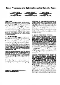
1.1 Column Stores After decades of only minor, incremental changes to the basic database architecture, a radically new design, column stores, started to gain traction in the years after 2005. Cstore [167] (commercialized as Vertica) and MonetDB/X100 [20] (commercialized as Vectorwise) are two influential systems that gained significant mind share during that time frame. The idea of organizing relations by column is, of course, much older [21]. Sybase IQ [125] and MonetDB [22] are two pioneering column stores that originated in the 1990s. Column stores are read-optimized and often used as data warehouses, i.e., nonoperational databases that ingest changes periodically (e.g., every night). In comparison with row stores, column stores have the obvious advantage that scans only need to read those attributes accessed by a particular query resulting in less I/O operations. A second advantage is that the query engine of a column store can be implemented in a much more CPU-efficient way: Column stores can amortize the interpretation overhead of the iterator model by processing batches of rows (“vector-at-a-time”), instead of working only on individual rows (“tuple-at-a-time”). The major database vendors have reacted to the changing landscape by combining multiple storage and query engines in their products. In Microsoft SQL Server, for example, users now can choose between the • traditional general-purpose row store,

1

1 Introduction

600,000

system Actian Vectorwise

queries per hour

Microsoft SQL Server Oracle 400,000

Sybase IQ

200,000

0 2002

2004

2006

2008

year

2010

2012

2014

2016

Figure 1.1: TPC-H single-machine performance for scale factor 1000 (1 TB) • a column store [100] for OnLine Analytical Processing (OLAP), and • in-memory storage optimized for Online transaction processing (OLTP) [37]. Each of these options comes with its own query processing model and specific performance characteristics, which must be carefully considered by the database administrator. The impact of column stores can be seen in Figure 1.1, which shows the performance on TPC-H, a widely used OLAP benchmark. Before 2011, multiple vendors competed for the TPC-H crown, with the lead changing from time to time between Oracle, Microsoft, and Sybase1 . This changed with the arrival of Actian Vectorwise in 2011, which disrupted the incremental “rat race” between the traditional vendors. The dominance of Vectorwise as official TPC-H leader lasted until 2014, when Microsoft submitted new results with their column store engine Apollo [100], which is currently the leading system.

1.2 Main-Memory Database Systems The lower CPU overhead of column store query engines was of only minor importance as long as data was mainly stored on disk (or even SSD). In 2000 one had to pay over 1

2

IBM submitted results for other scale factors, but not for scale factor 1000.

1.2 Main-Memory Database Systems 1000$ for 1 GB of DRAM2 . At these prices, any non-trivial database workload resulted in a significant number of disk I/O operations, and main-memory DBMSs—which were a research topic as early as the 1980s [50]—were still niche products. In 2008, with the same 1000$ one could already buy 100 GB of RAM3 . This rapid decrease in DRAM prices had consequences for the architecture of database management systems. Harizopoulos et al.’s paper from 2008 [63] showed that on the—suddenly very common—memory-resident OLTP workloads virtually all time was wasted on overhead like • buffer management, • locking, • latching, • heavy-weight logging, and • an inefficient implementation. The goal of any database system’s designer thus gradually shifted from minimizing the number of disk I/O operations to reducing CPU overhead and cache misses. This lead to a resurgence of research into main-memory database systems. The main idea behind main-memory DBMSs is to assume that all data fits into RAM and to optimize for CPU and cache efficiency. Using careful engineering and by making the right architectural decisions that take modern hardware into account, database systems can achieve orders of magnitude higher performance. Well-known mainmemory database systems include H-Store/VoltDB [83, 168], SAP HANA [43], Microsoft Hekaton [102], solidDB [118], Oracle TimesTen [95], Calvin [171], Silo [172], MemSQL, and HyPer [87]. The work described in this thesis has been done in the context of the HyPer project, which started in 2010 [86]. HyPer follows some of the design decisions of other mainmemory systems (e.g., no buffer manager, no locks, no latches, and (originally) command logging). To avoid fine-grained latches, HyPer also initially followed H-Store’s approach of relying on user-controlled, physical partitioning of the database to enable multi-threading. HyPer has, however, a number of features that distinguish it from many other mainmemory systems: From the very beginning, HyPer supported both OLTP and OLAP in the same database in order to make the physical separation between the transactional and data warehouse databases obsolete. Initially, HyPer used OS-supported snapshots [87], which were later replaced with a software-controlled Multi-Version 2 3

DRAM prices are taken from http://www.jcmit.com/memoryprice.htm. The cost continues to decline. At the time of writing, in 2016, the cost was around 4$ per GB.

3

1 Introduction Concurrency Control (MVCC) approach [143]. The second unique feature of HyPer is that, via the LLVM [104] compiler infrastructure, it compiles SQL queries and stored procedures to machine code [139]. Compilation avoids the interpretation overhead inherent in the iterator model and thereby enables extremely high performance. LLVM is a widely used open source compiler backend that can generate efficient machine code for many different target platforms, which makes this approach portable. In contrast to previous compilation approaches (e.g., [94]), HyPer compiles multiple relational operators from the same query pipeline into a single intertwined code fragment, which allows it to keep values in CPU registers for as long as possible. In terms of architecture, most column stores have converged to a similar design [1], which was pioneered by systems like Vectorwise [20] and Vertica [167]. In-memory OLTP systems, in contrast, show more architectural variety. Compilation is, however, becoming a common building block for OLTP systems, as can be observed by the use of compilation by HyPer [139], Hekaton [37], and MemSQL. Other high-performance systems like Silo [172] also implicitly assume (but do not yet implement) compilation, as the stored procedures are hand-written in C or C++ in these systems. In other areas like concurrency control (e.g., [172] vs. [98] vs. [143]), indexing (e.g., [108] vs. [129] vs. [114]), and logging (e.g., [127] vs. physiological) there is much more variety between the systems.

1.3 The Challenges of Modern Hardware Besides increasing main-memory sizes, a second important trend in the hardware landscape is the ever increasing number of cores. Figure 1.2 shows the number of cores for server CPUs4 . Over the entire time frame, the clock rate stayed between 2 GHz and 3 GHz and, as a result, single-threaded performance increased only very slowly (by single-digit percentages per year). Note that the graph only shows “real” cores for a single socket. Many servers have 2, 4, or even 8 sockets in a single system and each Intel core nowadays has 2-way HyperThreading. As a result, the affordable and commonly used 2-socket configurations will soon routinely have over 100 hardware threads in a single system. Memory bandwidth has largely kept up with the increasing number of cores and will reach over 100 GB/s per socket with Skylake EP. However, it is important to note that a single core can only utilize a small fraction of the available bandwidth, making effective parallelization essential. Long before the many-core revolution, high-end database servers often combined a handful of processors—connected by a shared memory bus—in a Symmetric MultiProcessing (SMP) system. Furthermore, database systems have, for a long time, been 4

4

The data is from https://en.wikipedia.org/wiki/List_of_Intel_Xeon_ microprocessors. For Broadwell EX and Skylake EP server CPUs we show estimates from the press as they were not yet released at the time of writing.

1.3 The Challenges of Modern Hardware 30

Skylake EP Broadwell EX

cores per CPU

Broadwell EP 20

Haswell EP Ivy Bridge EX Ivy Bridge EP Nehalem (Westmere EX)

10

Nehalem (Beckton) Sandy Bridge EP Core (Kentsfield) Core (Lynnfield)

1

NetBurst (Foster)

2000

NetBurst (Paxville)

2004

2008

year

2012

2016

Figure 1.2: Number of cores in Intel Xeon server processors (for the largest configuration in each microarchitecture) capable of executing queries concurrently by using appropriate locking and latching techniques. So one might reasonably ask if any fundamental changes to the database architecture are required at all. Modern hardware, however, has unique challenges not encountered in the past: Latches are expensive and prevent scaling. Traditional database systems use latches extensively to access shared data structures from concurrent threads. As long as disk I/O operations were frequent, the overhead of short-term latching was negligible. On modern hardware, however, even short-term, uncontested latches can be expensive and prevent scalability. The reason is that each latch acquisition causes cache line invalidations for all other cores. As we show experimentally, this effect often prevents scalability on multi-core CPUs. Intra-query parallelism is not optional any more. For a long time, many systems relied on parallelism from the “outside”, i.e., inter-query parallelism. With dozens or hundreds of cores, intra-query parallelism is not an optional optimization because many workloads simply do not have enough parallel query sessions. Without intraquery parallelism, the computational resources of modern servers lie dormant. The widely used PostgreSQL system, for example, will finally introduce (limited) intraquery parallelism in the upcoming version 9.6—20 years after the project started. Query engines should be designed with multi-core parallelism in mind. Some

5

1 Introduction commercial systems added support for intra-query parallelism a decade ago. This was often done by introducing “exchange” operators [52] that encapsulate parallelism without redesigning the actual operators. This pragmatic approach was sufficient at a time when the degree of parallelism in database servers was low (e.g., 10 threads). To get good scalability on systems with dozens of cores, the query processing algorithms should be redesigned from scratch with parallelism in mind. Database systems should take Non-Uniform Memory Architecture (NUMA) into account. In contrast to earlier SMP systems, where all processors shared a common memory bus, current systems are generally based on the Non-Uniform Memory Architecture (NUMA). In this architecture each processor has its own memory, but can transparently and cache-coherently access remote memory through an interconnect. Because remote memory accesses are more expensive than local accesses, NUMAaware data placement can improve performance considerably. Thus, database systems must optimize for NUMA to obtain optimal performance. Together, these changes explain why traditional systems (e.g., as described in [66]) cannot fully exploit the resources provided today’s commodity servers. To utilize modern hardware well, fundamental changes to core database components including storage, concurrency control, low-level synchronization, query processing, logging, etc. are necessary. Database systems specifically designed for modern hardware can be orders of magnitude faster than their predecessors.

1.4 Outline This thesis addresses the challenges enumerated above. The solutions were developed within a general-purpose, relational database system (HyPer) and most experiments measure end-to-end performance. Our contributions span the transaction processing, query processing, and query optimization components. In Chapter 2 we design a low-overhead, concurrent transaction processing engine based on Hardware Transactional Memory (HTM). Until recently, transactional memory— although a promising technique—suffered from the absence of an efficient hardware implementation. Since Intel introduced the Haswell microarchitecture hardware transactional memory is available in mainstream CPUs. HTM allows for efficient concurrent, atomic operations, which is also highly desirable in the context of databases. On the other hand, HTM has several limitations that, in general, prevent a one-to-one mapping of database transactions to HTM transactions. We devise several building blocks that can be used to exploit HTM in main-memory databases. We show that HTM allows one to achieve nearly lock-free processing of database transactions by carefully controlling the data layout and the access patterns. The HTM component is used for detecting the (infrequent) conflicts, which allows for an optimistic—and thus

6

1.4 Outline very low-overhead execution—of concurrent transactions. We evaluate our approach on a 4-core desktop and a 28-core server system and find that HTM indeed provides a scalable, powerful, and easy to use synchronization primitive. While Hardware Transactional Memory is easy to use and can offer good performance, it is not yet widespread. Therefore, Chapter 3 studies alternative low-overhead synchronization mechanisms for in-memory data structures. The traditional approach, fine-grained locking, does not scale on modern hardware. Lock-free data structures, in contrast, scale very well but are extremely difficult to implement and often require additional indirections. We argue for a middle ground, i.e., synchronization protocols that use locking, but only sparingly. We synchronize the Adaptive Radix Tree (ART) [108] using two such protocols, Optimistic Lock Coupling and Read-Optimized Write EXclusion (ROWEX). Both perform and scale very well while being much easier to implement than lock-free techniques. Chapter 4 describes the parallel and NUMA-aware query engine of HyPer, which scales up to dozens of cores. Our “morsel-driven” query execution framework, where scheduling becomes a fine-grained run-time task that is NUMA-aware. Morsel-driven query processing takes small fragments of input data (“morsels”) and schedules these to worker threads that run entire operator pipelines until the next pipeline-breaking operator. The degree of parallelism is not baked into the plan but can elastically change during query execution. The dispatcher can react to the execution speed of different morsels but also adjust resources dynamically in response to newly arriving queries in the workload. Furthermore, the dispatcher is aware of data locality of the NUMAlocal morsels and operator state, such that the great majority of executions takes place on NUMA-local memory. Our evaluation on the TPC-H and SSB benchmarks shows extremely high absolute performance and an average speedup of over 30 with 32 cores. Chapter 5 completes the description of HyPer’s query engine by proposing a design for the SQL:2003 window function operator. Window functions, also known as analytic OLAP functions, have been neglected in the research literature—despite being part of the SQL standard for more than a decade and being a widely-used feature. Window functions can elegantly express many useful queries about time series, ranking, percentiles, moving averages, and cumulative sums. Formulating such queries in plain SQL-92 is usually both cumbersome and inefficient. Our algorithm is optimized for high-performance main-memory database systems and has excellent performance on modern multi-core CPUs. We show how to fully parallelize all phases of the operator in order to effectively scale for arbitrary input distributions. The only thing more important for achieving low query response times than a fast and scalable query engine is query optimization. In Chapter 6 we shift our focus from the query engine to the query optimizer. Query optimization has been studied for decades, but most experiments were in the context of disk-based systems or were focused on individual query optimization components rather than end-to-end perfor-

7

1 Introduction mance. We introduce the Join Order Benchmark (JOB) and experimentally revisit the main components in the classic query optimizer architecture using a complex, realworld data set and realistic multi-join queries. We investigate the quality of industrialstrength cardinality estimators and find that all estimators routinely produce large errors. We further show that while estimates are essential for finding a good join order, query performance is unsatisfactory if the query engine relies too heavily on these estimates. Using another set of experiments that measure the impact of the cost model, we find that it has much less influence on query performance than the cardinality estimates. Finally, we investigate plan enumeration techniques comparing exhaustive dynamic programming with heuristic algorithms and find that exhaustive enumeration improves performance despite the sub-optimal cardinality estimates.

8

2 Exploiting Hardware Transactional Memory in Main-Memory Databases Parts of this chapter have previously been published in [109, 110].

2.1 Introduction The support for hardware transactional memory (HTM) in mainstream processors like Intel’s Haswell appears like a perfect fit for main-memory database systems. Transactional memory [69] is a very intriguing concept that allows for automatic atomic and concurrent execution of arbitrary code. Transactional memory allows for code that behaves quite similar to database transactions: transaction { a = a − 10; b = b + 10; } Transaction 1

transaction { c = c − 20; a = a + 20; } Transaction 2

Semantically, the code sections are executed atomically and in isolation from each other. In the case of runtime conflicts (i.e., read/write conflicts or write/write conflicts) a transaction might get aborted, undoing all changes performed so far. The transaction model is a very elegant and well understood idea that is much simpler than the classical alternative, namely fine-grained locking. Locking is much more difficult to formulate correctly. Fine-grained locking is error prone and can lead to deadlocks due to differences in locking order. Coarse-grained locking is simpler, but greatly reduces concurrency. Transactional memory avoids this problem by keeping track of read and write sets and thus by detecting conflicts on the memory access level. Starting with the Intel’s Haswell microarchitecture this is supported by hardware, which offers excellent performance.

11

2 Exploiting Hardware Transactional Memory in Main-Memory Databases Throughput

Overhead of HTM/TSO

ing

on rtiti l pa

.m opt

a anu M HT

serial execution Overhead SW versus HTM

2 PL

# Cores / Threads

Figure 2.1: HTM versus 2PL, sequential, partitioned

Figure 2.1 sketches the performance benefits of our HTM-based transaction manager in comparison to other concurrency control mechanisms that we investigated. For main-memory database applications the well-known Two Phase Locking scheme was shown to be inferior to serial execution [63]! However, serial execution cannot exploit the parallel compute power of modern multi-core CPUs. Under serial execution, scaling the throughput in proportion to the number of cores would require an optimal partitioning of the database such that transactions do not cross these boundaries. This allows for “embarrassingly” parallel execution—one thread within each partition. Unfortunately, this is often not possible in practice; therefore, the upper throughput curve “opt. manual partitioning” of Figure 2.1 is only of theoretical nature. HTM, however, comes very close to an optimal static partitioning scheme as its transaction processing can be viewed as an adaptive dynamic partitioning of the database according to the transactional access pattern. However, transactional memory is no panacea for transaction processing. First, database transactions also require properties like durability, which are beyond the scope of transactional memory. Second, all current hardware implementations of transactional memory are limited. For the Haswell microarchitecture, for example, the scope of a transaction is limited, because the read/write set, i.e., every cache line a transaction accesses, has to fit into the L1 cache with a capacity of 32KB. Furthermore, HTM transactions may fail due to a number of unexpected circumstances like collisions caused by cache associativity, hardware interrupts, etc. Therefore, it is, in general, not viable to map an entire database transaction to a single monolithic HTM transaction. In addition, one always needs a “slow path” to handle the pathological cases (e.g., associativity collisions). We therefore propose an architecture where transactional memory is used as a build-

12

2.1 Introduction

T1

T1 T2

T2

T3

T3

Figure 2.2: Schematic illustration of static partitioning (left) and concurrency control via HTM resulting in dynamic partitioning (right) ing block for assembling complex database transactions. Along the lines of the general philosophy of transactional memory we start executing transactions optimistically, using (nearly) no synchronization and thus running at full clock speed. By exploiting HTM we get many of the required checks for free, without complicating the database code, and can thus reach a much higher degree of parallelism than with classical locking or latching. In order to minimize the number of conflicts in the transactional memory component, we carefully control the data layout and the access patterns of the involved operations, which allows us to avoid explicit synchronization most of the time. Note that we explicitly do not assume that the database is partitioned in any way. In some cases, and in particular for the well-known TPC-C benchmark, the degree of parallelism can be improved greatly by partitioning the database at the schema level (using the warehouse attribute in the case of TPC-C). Such a static partitioning scheme is exemplified on the left-hand side of Figure 2.2. VoltDB for example makes use of static partitioning for parallelism [168]. But such a partitioning is hard to find in general, and users usually cannot be trusted to find perfect partitioning schemes [98]. In addition, there can always be transactions that cross partition boundaries, as illustrated by Figure 2.2. In the figure the horizontal axis represents time and the colored areas represent the read/write sets of transactions T1, T2, and T3. The read/write sets do not overlap, but nevertheless there is no static partitioning scheme (horizontal line) that isolates the transactions. These transactions have to be isolated with a serial (or locking-based) approach as the static partitioning scheme cannot guarantee their isolation. If available, we could still exploit partitioning information in our HTM approach, of course, as then conflicts would be even more unlikely. But we explicitly do not assume the presence of such a static partitioning scheme and rely on the implicit adaptive partitioning of the transactions as sketched on the right-hand side of Figure 2.2. The rest of this chapter is structured as follows: First, we discuss the different alternatives for concurrency control within database systems in Section 2.2. Then, we

13

2 Exploiting Hardware Transactional Memory in Main-Memory Databases synchronization method 2PL serial execution manually partitioned, serial

1 thread 50,541 129,937 119,232

4 threads 108,756 369,549

Table 2.1: Transaction rates for various synchronization methods in HyPer discuss the advantages and limitations of hardware transactional memory in Section 2.3 and Section 2.4. In Section 2.5, we present our transaction manager, which uses hardware transactional memory as a building block for highly concurrent transaction execution. After that, we explain in Section 2.6 an HTM-friendly data layout which minimizes false conflicts. Experimental results are explained in Section 2.7. Finally, after presenting related work in Section 2.8, we summarize this chapter in Section 2.9.

2.2 Background and Motivation As databases are expected to offer ACID transactions, they have to implement a mechanism to synchronize concurrent transactions. The traditional concurrency control method used in most database systems is some variant of two-phase locking (2PL) [178]. Before accessing a database item (tuple, page, etc.), the transaction acquires a lock in the appropriate lock mode (shared, exclusive, etc.). Conflicting operations, i.e., conflicting lock requests, implicitly order transactions relative to each other and thus ensure serializability. In the past this model worked very well. Concurrent transaction execution was necessary to hide I/O latency, and the costs for checking locks was negligible compared to the processing costs in disk-based systems. However, this has changed in modern systems, where large parts of the data are kept in main memory, and where query processing is increasingly CPU bound. In such a setup, lock-based synchronization constitutes a significant fraction of the total execution time, in some cases even dominates the processing [63, 134]. This observation has motivated some main-memory based systems to adopt a serial execution model [63]: Instead of expensive synchronization, all transactions are executed serially, eliminating any need for synchronization. And as a main-memory based system does not have to hide I/O latency, such a model works very well for short, OLTP-style transactions. Table 2.1 shows TPC-C transaction rates under these two models. We used HyPer [87] as the basis for the experiments. The serial execution mode easily outperforms 2PL. Due to the inherent overhead of maintaining a synchronized lock manager in 2PL, serial execution achieves 2.6 times the transaction rate of 2PL. This is a strong argument in favor of the serial execution mode proposed by [63]. On the other hand, the fig-

14

2.2 Background and Motivation ure also shows the weakness of serial execution: Increasing the degree of parallelism in 2PL increases the transaction rate. Admittedly the effect is relatively minor in the TPC-C setting, using 4 threads results in a speedup of only 2, but there still is an effect. Serial execution cannot make use of additional threads, and thus the transaction rate remains constant. As the number of cores in modern systems grows while singlethreaded performance stagnates, this becomes more and more of a problem. Systems like H-Store/VoltDB [168] or HyPer [87] tried to solve this problem by partitioning the data. Both systems would partition the TPC-C workload along the warehouse attribute, and would then execute all transactions concurrently that operate on separate warehouses. If transactions access more than one warehouse, the system falls back to the serial execution model. In the TPC-C benchmark this occurs for about 11% of the transactions. Nevertheless, this model works relatively well for TPC-C, as shown in Figure 2.1, where it is about 3 times faster than serial execution for 4 threads. But it is not very satisfying to depend on static partitioning. First of all, it needs human intervention. The database administrator has to specify how the data should be partitioned; HyPer has no automatic mechanism for this, whereas in H-Store there were attempts to derive such partitioning schemes automatically, e.g., Schism [34]. But, as mentioned by Larson et al. [98], a good partitioning scheme is often hard to find, in particular when workloads may shift over time. For TPC-C the partitioning schema is obvious—as it was (artificially) specified as a schema tree—but for other schemata it is not. Second, the partitioning scheme breaks if transactions frequently cross their partition boundaries. For TPC-C this is not much of a problem, as only relatively few transactions cross partition boundaries and the workload does not change, but in general it is hard to find a partitioning scheme that fits a complex workload well. And it is important to note that a partition-crossing transaction does not necessarily conflict with any other transaction! In the static partitioning execution model two transactions will be serialized if they access the same partition, even if the data items they access are completely distinct. This is highlighted in Figure 2.2 where all three transactions on the left-hand side are viewed as potentially conflicting as they (occasionally) cross their partition boundaries. As this state of the art is not very satisfying, we will in the following develop a synchronization mechanism that is as fine-grained as 2PL and, in terms of overhead, nearly as cheap as serial execution. With our HTM-supported, dynamically-partitioned execution model the transactions shown on the right-hand side of Figure 2.2 are executed in parallel without conflicts as their read/write-sets do not overlap. Note that in this chapter we concentrate on relatively short, non-interactive transactions. The methods we propose are not designed for transactions that touch millions of tuples or that wait minutes for user interaction. In HyPer such long-running transactions are moved into a snapshot with snapshot-isolation semantics [87, 134, 143]. As these snapshots are maintained automatically by the OS, there is no interaction be-

15

2 Exploiting Hardware Transactional Memory in Main-Memory Databases tween these long-running transactions and the shorter transactions we consider here. In general, any system that adopts our techniques will benefit from a separate snapshotting mechanism to avoid the conflicts with long-running transactions, such as OLAP queries and interactive transactions.

2.3 Transactional Memory Traditional synchronization mechanisms are usually implemented using some form of mutual exclusion (mutex). For 2PL, the DBMS maintains a lock structure that keeps track of all currently held locks. As this lock structure is continuously updated by concurrent transactions, the structure itself is protected by one (or more) mutexes [58]. On top of this, the locks themselves provide a kind of mutual exclusion mechanism, and block a transaction if needed. The problem with locks is that they are difficult to use effectively. In particular, finding the right lock granularity is difficult. Coarse locks are cheap, but limit concurrency. Fine-grained locks allow for more concurrency, but are more expensive and can lead to deadlocks. For quite some time now, transactional memory has been proposed as an alternative to fine grained locking [69]. The key idea behind transactional memory is that a number of operations can be combined into a transaction, which is then executed atomically. Consider the following small code fragment for transferring money from one account to another account (using GCC syntax): transfer(from,to,amount) transaction atomic { account[from]-=amount; account[to]+=amount; } The code inside the atomic block is guaranteed to be executed atomically, and in isolation. In practice, the transactional memory observes the read set and write set of transactions, and executes transactions concurrently as long as the sets do not conflict. Thus, transfers can be executed concurrently as long as they affect different accounts, they are only serialized if they touch a common account. This behavior is very hard to emulate using locks. Fine-grained locking would allow for high concurrency, too, but would deadlock if accounts are accessed in opposite order. Transactional memory solves this problem elegantly using speculation (and conflict detection). Transactional memory has been around for a while, but has usually been implemented as Software Transactional Memory (STM), which implements transactions on the programming-language level. Although STM does remove the complexity of lock

16

2.3 Transactional Memory maintenance, it causes a significant slowdown during execution and thus had limited practical impact [28].

2.3.1 Hardware Support for Transactional Memory This changed with the Haswell microarchitecture from Intel, which offers Hardware Transactional Memory [73]. Note that Haswell was not the first CPU with hardware support for transactional memory, for example IBM’s Blue Gene/Q supercomputers [176] and System z mainframes [76] offered it before, but it is the first mainstream CPU to implement HTM. And in hardware, transactional memory can be implemented much more efficiently than in software: Haswell uses its highly optimized cache coherence protocol, which is needed for all multi-core processors anyway, to track read and write set collisions [155]. Therefore, Haswell offers HTM nearly for free. Even though HTM is very efficient, there are also some restrictions. First of all, the size of a hardware transaction is limited. For the Haswell microarchitecture it is limited to the size of the L1 cache, which is 32 KB. This implies that, in general, it is not possible to simply execute a database transaction as one monolithic HTM transaction. Even medium-sized database transactions would be too large. Second, in the case of conflicts, the transaction fails. In this case the CPU undoes all changes, and then reports an error that the application has to handle. And finally, a transaction might fail due to spurious hardware implementation details like cache associativity limits, interrupts, etc. Some of these failure modes are documented by Intel, while others are not. So, even though in most cases HTM will work fine, there is no guarantee that a transaction will ever succeed (if executed as an HTM transaction). Therefore, Intel proposes (and explicitly supports by specific instructions) using transactional memory for lock elision [155]. Conceptually, this results in code like the following: transfer(from,to,amount) atomic-elide-lock (lock) { account[from]-=amount; account[to]+=amount; } Here, we still have a lock, but ideally the lock is not used at all—it is elided. When the code is executed, the CPU starts an HTM transaction, but does not acquire the lock as shown on the left-hand side of Figure 2.3. Only when there is a conflict the transaction rolls back, acquires the lock, and is then executed non-transactionally. The right-hand side of Figure 2.3 shows the fallback mechanism to exclusive serial execution, which is controlled via the (previously elided) lock. This lock elision mechanism has two effects. First, ideally, locks are never acquired and transactions are executed

17

2 Exploiting Hardware Transactional Memory in Main-Memory Databases T1

T2

T1

Lock

T2

Lock

T2

T3

Lock

T1

optimistic parallel execution

validation fails

serial execution

Figure 2.3: Lock elision (left), conflict (middle), and serial execution (right) concurrently as much as possible. Second, if there is an abort due to a conflict or hardware-limitation, there is a “slow path” available that is guaranteed to succeed.

2.3.2 Caches and Cache Coherency Even though Intel generally does not publish internal implementation details, Intel did specify two important facts about Haswell’s HTM feature [155]: • The cache coherency protocol is used to detect transactional conflicts. • The L1 cache serves as a transactional buffer. Therefore, it is crucial to understand Intel’s cache architecture and coherency protocol. Because of the divergence of DRAM and CPU speed, modern CPUs have multiple caches in order to accelerate memory accesses. Intel’s cache architecture is shown in Figure 2.4, and consists of a local L1 cache (32 KB), a local L2 cache (256 KB), and a shared L3 cache (2-45 MB). All caches use 64 byte cache blocks (lines) and all caches are transparent, i.e., programs have the illusion of having only one large main memory. Because on multi-core CPUs each core generally has at least one local cache, a cache coherency protocol is required to maintain this illusion. Most CPU vendors, including Intel and AMD, use extensions of the well-known MESI protocol [67]. The name of the protocol derives from the four states that each cache line can be in (Modified, Exclusive, Shared, or Invalid). To keep multiple caches coherent, the caches have means of intercepting (“snooping”) each other’s load and store requests. For example, if a core writes to a cache line which is stored in multiple caches (Shared state), the state must change to Modified in the local cache and all

18

2.3 Transactional Memory

Core 0 L1

32KB

Core 1 L2

256KB

L1

Core 2 L2

32KB

256KB

L1

32KB

Core 3 L2

256KB

L1

32KB

L2

256KB

interconnect

(allows snooping and signalling)

copy of core 0 cache

memory controller


L3 cache copy of core 2 cache


Figure 2.4: Intel cache architecture copies in remote caches must be invalidated (Invalid state). This logic is implemented in hardware using the cache controller of the shared L3 cache that acts as a central component where all coherency traffic and all DRAM requests pass through. The key insight that allows for an efficient HTM implementation is that the L1 cache can be used as a local buffer. All transactionally read or written cache lines are marked and the propagation of changes to other caches or main memory is prevented until the transaction commits. Read/write and write/write conflicts are detected by using the same snooping logic that is used to keep the caches coherent. And since the MESI protocol is always active and commits/aborts require no inter-core coordination, transactional execution on Haswell CPUs incurs almost no overhead. The drawback is that the transaction size is limited to the L1 cache. This is fundamentally different from IBM’s Blue Gene/Q architecture, which allows for up to 20 MB per transaction using a multi-versioned L2 cache, but has relatively large runtime overhead [176]. Besides the nominal size of the L1 cache, another limiting factor for the maximum transaction size is cache associativity. Caches are segmented into sets of cache lines in order to speed up lookup and to allow for an efficient implementation of the pseudoLRU replacement strategy (in hardware). Haswell’s L1 cache is 8-way associative, i.e., each cache set has 8 entries. This has direct consequences for HTM, because all transactionally read or written cache lines must be marked and kept in the L1 cache until commit or abort. Therefore, when a transaction writes to 9 cache lines that happen to reside in the same cache set, the transaction is aborted. And since the mapping from memory address to cache set is deterministic (bits 7-12 of the address are used), restarting the transaction does not help, and an alternative fallback path is necessary for forward progress. In practice, bits 7-12 of memory addresses are fairly random, and aborts of very

19

2 Exploiting Hardware Transactional Memory in Main-Memory Databases

abort probability

100% 75% 50% 25% 0% 0

8KB

16KB

transaction size

24KB

32KB

Figure 2.5: Aborts from random memory writes

small transactions are unlikely. Nevertheless, Figure 2.5 shows that the abort probability quickly rises when more than 128 random cache lines (only about one quarter of the L1 cache) are accessed1 . This surprising fact is caused by a statistical phenomenon related to the birthday paradox: For example with a transaction size of 16 KB, for any one cache set it is quite unlikely that it contains more than 8 entries. However, at the same time, it is likely that at least one cache set exceeds this limit. The hardware ensures that the eviction of a cache line that has been accessed in an uncommitted transaction leads to a failure of this transaction, as it would otherwise become impossible to detect conflicting writes to this cache line. The previous experiment was performed with accesses to memory addresses fully covered by the translation lookaside buffer (TLB). TLB misses do not immediately cause transactions to abort, because, on x86 CPUs, the page table lookup is performed by the hardware (and not the operating system). However, TLB misses do increase the abort probability, as they cause additional memory accesses during page table walks. Besides memory accesses, another important reason for transactional aborts is interrupts. Such events are unavoidable in practice and limit the maximum duration of transactions. Figure 2.6 shows that transactions that take more than 1 million CPU cycles (about 0.3 ms) will likely be aborted. This happens due to interrupts and even if these transaction do not execute any memory operations. These results clearly show that Haswell’s HTM implementation cannot be used for long-running transactions but is designed for short critical sections. Despite these limitations we found that Haswell’s HTM implementation offers excellent scalability as long as transactions are short and free of conflicts with other transactions. 1

The experiments in this section were performed on an Intel i5 4670T.

20

2.4 Synchronization on Many-Core CPUs

abort probability

100% 75% 50% 25% 0% 10K

100K

1M

transaction duration in cycles (log scale)

10M

Figure 2.6: Aborts from transaction duration

2.4 Synchronization on Many-Core CPUs To execute transactional workloads, a DBMS must provide (1) high-level concurrency control to logically isolate transactions, and (2) a low-level synchronization mechanism to prevent concurrent threads from corrupting internal data structures. Both aspects are very important, as each of them may prevent scalability. In this section we focus on the low-level synchronization aspect, before describing our concurrency control scheme in Section 2.5. We experimentally evaluate HTM on a Haswell system with 28 cores and compare it with common synchronization alternatives like latching. The experiments in this section use a Haswell EP system with two Intel E5-2697 v3 processors that are connected through an internal CPU interconnect, which Intel calls QuickPath Interconnect (QPI). The processor is depicted in Figure 2.7 and has 14 cores, i.e., in total, the system has 28 cores (56 HyperThreads). The figure also shows that the CPU has two internal communication rings that connect cores and 2.5 MB slices of the L3 cache. An internal link connects these two rings, but is not to be confused with the QPI interconnect that connects the two sockets of the system. The system supports two modes, which can be selected in the systems’ BIOS: • The hardware can hide the internal ring internal structure, i.e., our two-socket system would expose two NUMA nodes with 14 cores each. • In the “cluster on die” configuration each internal ring is exposed as a separate NUMA node, i.e., our two-socket system has four NUMA nodes with 7 cores each. Using the first setting, each socket has 35 MB of L3 cache but higher latency, because an L3 access often needs to use the internal link. The cluster-on-die configuration,

21

2 Exploiting Hardware Transactional Memory in Main-Memory Databases memory controller internal link (to other ring)

core 0 L3 core 1 L3 core 2 L3 core 3 L3

memory controller

L3 core 4

core 7 L3

L3 core 5

core 8 L3

L3 core 6

core 9 L3

L3 core 10 L3 core 11 L3 core 12 L3 core 13

QPI interconnect (to other socket)

Figure 2.7: Intel E5-2697 v3 which we use for all experiments, has lower latency and 17.5 MB of cache per “cluster”, each of which consists of 7 threads. As has been widely reported, all Haswell systems shipped so far, including our system, contain a hardware bug in the Transactional Synchronization Extensions (TSX). According to Intel, this bug occurs “under a complex set of internal timing conditions and system events“. We have not encountered this bug during our tests. It seems to be very rare, as evidenced by the fact that it took Intel over a year to even find it. Furthermore, Intel has announced that the bug will be fixed in upcoming CPU generations.

2.4.1 The Perils of Latching Traditionally, database systems synchronize concurrent access to internal data structures (e.g., index structures) with latches. Internally, a latch is implemented using atomic operations like compare-and-swap, which allow one to exclude other threads from entering a critical section. To increase concurrency, read/write latches are often used, which, at any time, allow multiple concurrent readers but only a single writer. Unfortunately, latches do not scale on modern hardware as Figure 2.8, which performs lookups in an Adaptive Radix Tree [108], shows. The curve labeled as “rw spin lock” shows the performance when we add a single read/write latch at the root node of the tree2 . With many cores, using no synchronization is faster by an order of magnitude! Note that this happens on a read-only workload without any logical contention, and is not caused by a bad latch implementation3 : When we replace the latch with a sin2

In reality, one would use lock-coupling and one latch at each node, so the performance would be even worse. 3 We used spin rw mutex from the Intel Thread Building Blocks library.

22

2.4 Synchronization on Many-Core CPUs

no sync

M ops/s

75

50 atomic

25

rw_spin_lock

0 1

14

28

threads

42

56

Figure 2.8: Lookups in a search tree with 64M entries gle atomic integer increment operation, which is the cheapest possible atomic write operation, the scalability is almost as bad as with the latch. The reason for this behavior is that to acquire a latch, CPUs must acquire exclusive access to the cache line where the latch is stored. As a result, threads compete for this cache line, and every time the latch is acquired, all copies of this cache line are invalidated in all other cores (“cache line ping-pong”). This happens even with atomic operations like atomic increment, although this operation never fails in contrast to compare-and-swap, which is usually used to implement latches. Note that latches also result in some overhead during single-threaded execution, but this overhead is much lower as the latch cache line is not continuously invalidated. Cache line ping-pong is often the underlying problem that prevents systems from scaling on modern multi-core CPUs.

2.4.2 Latch-Free Data Structures As a reaction to the bad scalability of latching some systems use latch-free data structures. Microsoft’s in-memory transaction engine Hekaton, for example, uses a lockfree hash table and the latch-free Bw-Tree [114] as index structures. In the latch-free approach read accesses can proceed in a non-blocking fashion without acquiring any latches and without waiting. Writes must make sure that any modification is performed using a sequence of atomic operations while ensuring that simultaneous reads are not disturbed. Since readers do not perform writes to global memory locations, this approach generally results in very good scalability for workloads that mostly consist of reads. However, latch-free data structure have a number of disadvantages:

23

2 Exploiting Hardware Transactional Memory in Main-Memory Databases • The main difficulty is that, until the availability of Hardware Transactional Memory, CPUs provided only very primitive atomic operations like compare-andswap, and a handful of integer operations. Synchronizing any non-trivial data structure with this limited tool set is very difficult and bug-prone, and for many efficient data structures, including the Adaptive Radix Tree, so far, no latch-free synchronization protocol exists. In practice, data structures must be designed with latch-freedom in mind, and the available atomic operations restrict the design space considerably. • And even if one succeeds in designing a latch-free data structure, this may not guarantee optimal performance. The reason is that, usually, additional indirections must be introduced, which often add significant overhead in comparison with an unsynchronized variant of the data structure. The Bw-Tree [114], for example, requires a page table indirection, which must be used on each node access and incurs additional cache misses. • Finally, memory reclamation is an additional problem. Without latches, a thread can never be sure when it is safe to reclaim memory, because concurrent readers might still be active. An additional mechanism (e.g., epoch-based reclamation), which again adds some overhead, is required to allow for safe memory reclamation. For these reasons, we believe that it is neither realistic nor desirable to replace all the custom data structures used by database systems with latch-free variants. Hardware Transactional Memory offers an easy to use, and, as we will show, efficient alternative. In particular, HTM has no memory reclamation issues and one can simply wrap each data structure access in a hardware transaction. This means that data structures can be designed without spending too much thought on how to synchronize them—though some understanding of how HTM works and its limitations is certainly beneficial.

2.4.3 Hardware Transactional Memory on Many-Core Systems Figure 2.9 shows the performance of HTM on the same read-only workload as Figure 2.8. We compare different lock elision approaches (with a single global, elided latch), and we again show the performance without synchronization as a theoretical upper bound. Surprisingly, the built-in hardware lock elision (HLE) instructions do not scale well when more than 4 cores are used. The internal implementation of HLE is not disclosed, but the reason for its bad performance is likely an insufficient number of restarts. As we have mentioned previously, a transaction can abort spuriously for many reasons. A transaction should therefore retry a number of times instead of giving up immediately and acquiring the fallback latch. The graph shows that for a read-only

24

2.4 Synchronization on Many-Core CPUs no sync

M ops/s

75

7 or more restarts

50

3 restarts

25

2 restarts

built-in HLE

1 restarts 0 restarts

0 1

14

28

threads

42

56

Figure 2.9: Lookups in an ART index with 64M integer entries under a varying number of HTM restarts workload, restarting at least 7 times is necessary, though a higher number of restarts also works fine. Therefore, we implemented lock elision manually using the restricted transactional memory (RTM) primitives xbegin, xend, xabort, but with a configurable number of restarts. Figure 2.10 shows the state diagram of our implementation. Initially the optimistic path (left-hand side of the diagram) is taken, i.e., the critical section is simply wrapped by xbegin and xend instructions. If an abort happens in the critical section (e.g., due to a read/write conflict), the transaction is restarted a number of times before falling back to actual latch acquisition (right-hand side of the diagram). Furthermore, transactions add the latch to their read set and only proceed into the critical section optimistically when the latch is free. When it is not free, this means that another thread is in the critical section exclusively (e.g., due to code that cannot succeed transactionally). In this case, the transaction has to wait for the latch to become free, but can then continue to proceed optimistically using RTM. Note that all this logic is completely hidden behind a typical acquire/release latch interface, and—once it has been implemented—it can be used just as easily as ordinary latches or Itel’s Hardware Lock Elision instructions. Furthermore, as Diegues and Romano [39] have shown, the configuration parameters of the restart strategy can be determined dynamically. When sufficient restarts are used, the overhead of HTM in comparison to unsynchronized access is quite low. Furthermore, we found that HyperThreading improves performance for many workloads, though one has to keep in mind that because each pair of HyperThreads shares one L1 cache, the effective maximum working set size is halved, so there might be workloads where it is beneficial to avoid this feature. Good scalability on read-only workloads should be expected, because only infre-

25


optimistic xbegin()

fallback

latch is not free

latch is free

acquire latch

xabort()

latch is not free

ma x

ma latch is free

critical section

ret

x

ab t

or

success

pause

ry=

ry
amount UPDATE account SET balance=balance-amount WHERE id=from; UPDATE account SET balance=balance+amount WHERE id=to; COMMIT TRANSACTION;

acquireHTMLatch(account.latch) tid=uniqueIndexLookup(account, ...) verifyWrite(account, tid) logUpdate(account, tid, ...) updateTuple(account, tid, ...) releaseHTMLatch(account.latch)

tuple=getTuple(account, tid) if ((tuple.writeTS>safeTSand tuple.writeTS!=now) OR (tuple.readTS>safeTS and tuple.readTS!=now)) { releaseHTMLatch(accout.latch) rollback() handleTSConflict() } tuple.writeTS=max(tuple.writeTS, now)

Figure 2.14: Implementing database transactions with timestamps and lock elision compensation [133]. Then, the transaction is executed serially by using a global lock, rolling the log forward again. This requires logical logging and non-interactive transactions, as we cannot roll a user action backward or forward. We use snapshots to isolate interactive transactions from the rest of the system [134]. The fallback to serial execution ensures forward progress, because in serial execution a transaction will never fail due to conflicts. Note that it is often beneficial to optimistically restart the transaction a number of times instead of resorting to serial execution immediately, as serial execution is very pessimistic and prevents parallelism. Figure 2.14 details the implementation of a database transaction using lock elision and timestamps. The splitting of stored procedures into smaller HTM transactions is fully automatic (done by our compiler) and transparent for the programmer. As shown in the pseudo code, queries or updates (within a database transaction) that access a single tuple through a unique index are directly translated into a single HTM transaction. Larger statements like range scans should be split into multiple HTM transactions, e.g., one for each accessed tuple. The index lookup and timestamp checks are protected using an elided latch, which avoids latching the index structures themselves. The implementation of the HTM latch is described in Section 2.4.3.

2.5.3 Optimizations How the transaction manager handles timestamp conflicts is very important for performance. If the conflict is only caused by the conservatism of the safe timestamp (i.e.,

32

2.5 HTM-Supported Transaction Management regular TSO would have no conflict), it is sometimes possible to avoid rolling back the transaction. If the conflicting transaction has a smaller timestamp and has already finished, the apparent conflict can be ignored. This optimization is possible because the safe timestamp cannot overtake a currently running transaction’s timestamp. As mentioned before, it is often beneficial to restart an aborted transaction a number of times, instead of immediately falling back to serial execution. In order for the restart to succeed, the safe timestamp must have advanced past the conflict timestamp. Since this timestamp is available (it triggered the abort), the transaction can wait, while periodically recomputing the safe timestamp until it has advanced sufficiently. Then the transaction can be restarted with a new timestamp and safe timestamp. The disadvantage of this approach is that during this waiting period no useful work is performed by the thread. A more effective strategy is to suspend the aborted transaction and execute other transactions instead. Once the safe timestamp has advanced past the conflicting transaction’s timestamp that transaction can be resumed. This strategy avoids wasteful waiting. We found rollback and re-execution to be quite cheap because the accessed data is often in cache. Therefore, our implementation immediately performs an abort after a timestamp conflict, as shown in Figure 2.14, and executes other transactions instead, until the safe timestamp has sufficiently advanced. We additionally limit the number of times a transaction is restarted before falling back to serial execution—thus ensuring forward progress. While our description here and also our initial implementation uses both read and write timestamps, it is possible to avoid read timestamps. Read timestamps are a bit unfortunate, as they can cause “false” HTM conflicts due to parallel timestamp updates, even though the read operations themselves would not conflict. Semantically the read timestamps are used to detect if a tuple has already been read by a newer transaction, which prohibits updates by older transactions (as they would destroy serializability). However, the read timestamps can be avoided by keeping track of the write timestamps of all data items accessed (read or written) by a certain transaction. Then, at commit time, the transaction re-examines the write timestamps of all data items and aborts if any one of them has changed [45], ensuring serializability. We plan to implement this technique in future work, and expect to get even better performance in the case of read hotspots. It is illustrative to compare our scheme to software transactional memory (STM) systems. Indeed, our scheme can be considered an HTM-supported implementation of STM. However, we get significantly better performance than pure STM by exploiting DBMS domain knowledge. For example, index structures are protected from concurrent modifications by the HTM transaction, but are not tracked with timestamps, as full transaction isolation would in fact be undesirable there. This is similar to B-tree latching in disk-based systems—however, at minimal cost. The indexed tuples themselves

33

2 Exploiting Hardware Transactional Memory in Main-Memory Databases are isolated via timestamps to ensure serializable transaction behavior. Note further that our interpretation of timestamps is different from regular TSO [27]: Instead of deciding about transaction success and failure as in TSO, we use timestamps to detect intersecting read/write sets, just like the hardware itself for the HTM part. In the case of conflicts, we do not abort the transaction or retry with a new timestamp an indefinite number of times, but fall back to the more restrictive sequential execution mode that ensures forward progress and guarantees the eventual success of every transaction.

2.6 HTM-Friendly Data Storage Transactional memory synchronizes concurrent accesses by tracking read and write sets. This avoids the need for fine-grained locking and greatly improves concurrency as long as objects at different memory addresses are accessed. However, because HTM usually tracks accesses at cache line granularity, false conflicts may occur. For example, if the two data items A and B happen to be stored in a single cache line, a write to A causes a conflict with B. This conflict would not have occurred if each data item had its own dedicated lock. Therefore, HTM presents additional challenges for database systems that must be tackled in order to efficiently utilize this feature.

2.6.1 Data Storage with Zone Segmentation With a straightforward contiguous main-memory data layout, which is illustrated on the left-hand side of Figure 2.15, an insert into a relation results in appending the tuple to the end of the relation. It is clear that such a layout does not allow concurrent insertions, because each insert writes to the end of the relation. Additionally, all inserts will try to increment some variable N which counts the number of tuples. The memory location at the end of the table and the counter N are hotspots causing concurrent inserts to fail. In order to allow for concurrent inserts, we use multiple zones per relation, as shown on the right-hand side of Figure 2.15. Each relation has a constant number of these zones, e.g., two times the number of hardware threads. A random zone number is assigned to each transaction, and all inserts of that transaction use this local zone. The same zone number is also used for inserts into other relations. Therefore, with an appropriately chosen number of zones, concurrent inserts can proceed with only a small conflict probability, even if many relations are affected. Besides the relatively small insert zones, each relation has a main zone where, for large relations, most tuples are stored. The boundary is stored in a counter N . For each zone i, the base Bi and the next insert position Ni are maintained. When a zone becomes full (i.e., when Ni reaches Bi+1 ), it is collapsed into the neighboring zone, and a new zone at the end of the table

34

2.6 HTM-Friendly Data Storage

main Ti: insert N Tj: insert free

Ti: insert

N B1 N1 B2 N2

free

free

Zone1 Zone2 Tj: insert

Figure 2.15: Avoiding hotspots by zone segmentation is created. Note that no tuples are copied and the tuple identifiers do not change, only the sizes of zones need to be adjusted. As a consequence, collapsing zones does not affect concurrent access to the tuples. Eventually, the insert zones are collapsed with the large contiguous main area. For a main-memory databases this guarantees very fast scan performance at clock speed during query processing. The counters Ni and Bi should be stored in separate cache lines for each zone, as otherwise unnecessary conflicts occur while updating these values.

2.6.2 Index Structures Besides the logical isolation of transactions using 2PL or TSO, database systems must isolate concurrent accesses to index structures. In principle, any data structure can be synchronized using HTM by simply wrapping each access in a transaction. In this section we first discuss how scalability can be improved by avoiding some common types of conflicts, before showing that HTM has much better performance than traditional index synchronization via fine-grained latches. One common problem is that indexes sometimes have a counter that stores the number of key/value pairs and prevents concurrent modifications. Fortunately, this counter is often not needed and can be removed. For data structures that allocate small memory chunks, another source of HTM conflicts is memory allocation. This problem can be solved by using an allocator that has a thread-local buffer. Surrogate primary keys are usually implemented as ascending integer sequences. For tree-based index structures, which maintain their data in sorted order, this causes HTM conflicts because all concurrent inserts try to access memory locations in the same vicinity, as illustrated on the left-hand side of Figure 2.16. This problem is very similar to the problem of concurrently inserting values into a table discussed above, and

35

2 Exploiting Hardware Transactional Memory in Main-Memory Databases decluster

Tree-based Index

cache line collisions

Tree-based Index

Figure 2.16: Declustering surrogate key generation indeed the solution is similar: If permitted by the application, the integer sequence is partitioned into multiple constant-sized chunks and values are handed out from one of the chunks depending on the transactions’ zone number. This prevents interference of parallel index tree insertions as they are spread across different memory locations—as shown on the right of Figure 2.16. Once all values from a chunk are exhausted, the next set of integers is assigned to it. Note that hash tables are not affected by this problem because the use of a hash function results in a random access pattern which leads to a low conflict probability. But of course, as a direct consequence of this randomization, hash tables do not support range scans.

2.7 Evaluation For most experiments we used an Intel i5 4670T Haswell processor with 4 cores, 6 MB shared L3 cache, and full HTM support through the Intel Transactional Synchronization Extensions. The maximum clock rate is 3.3 GHz, but can only be achieved when only one core is fully utilized. When utilizing all cores, we measured a sustained clock rate of 2.9 GHz. By default, HyPer uses serial execution similar to VoltDB [168]; multiple threads are only used if the schema has been partitioned by human intervention. In the following we will call these execution modes serial and partitioned. Note that the partitioned mode used by HyPer (as in other systems) is somewhat cheating, since the partitioning scheme has to be explicitly provided by a human, and a good partitioning scheme is hard to find in general. In addition to these execution modes we included a 2PL implementation, described in [134], as baseline for comparisons to standard database systems, and the hardware transactional memory approach (HTM) proposed here. We also include TSO with coarse-grained latches (TSO) instead of HTM to show that TSO alone is not sufficient for good performance. For most experiments we used the well-known TPC-C benchmark as basis (without “think times”, the only deviation from the benchmark rules). We set the number of warehouses to 32, and for the partitioning experiments the strategy was to partition both the data and the transactions by the main warehouse. We used the Adaptive Radix Tree [108] as index structure, although the scalability is similar with hash tables and

36

2.7 Evaluation

400,000 HTM

transactions per second

partitioned TSO

300,000

serial 2PL 200,000

100,000

0 1

2

threads

3

4

Figure 2.17: Scalability of TPC-C on desktop system red-black trees. In the following, we first look at scalability results for TPC-C and then study the interaction with HTM in microbenchmarks.

2.7.1 TPC-C Results In the first experiment, we ran TPC-C and varied the number of threads up to the number of available cores. The results are shown in Figure 2.17 and reveal the following: First, classical 2PL is clearly inferior to all other approaches. Its overhead is too high, and it is even dominated by single-threaded serial execution. The latching-based TSO approach has less overhead than 2PL, but does not scale because the coarse-grained (relation-level) latches severely limit concurrency. Both the partitioned scheme and HTM scale very well, with partitioning being slightly faster. But note that this is a comparison of a human-assisted approach with a fully automatic approach. Furthermore, the partitioning approach works so well only because TPC-C is “embarrassingly partitionable” in this low-thread setup, as we will see in the next experiment. The reason that partitioning copes well with TPC-C is that most transactions stay within a single partition. By default, about 11% of all transactions cross partition boundaries (and therefore require serial execution to prevent collisions in a lock-free system). The performance depends crucially on the ability of transactions to stay within one partition. As shown in Figure 2.18, varying the percentage of partitioncrossing transactions has a very deteriorating effect on the partitioning approach, while the other transaction managers are largely unaffected because, in the case of TPC-C, partition-crossing does not mean conflicting. Therefore, picking the right partitioning

37


400,000

2PL


HTM partitioned 300,000

serial TSO

200,000

100,000

0 0%

25%

50%

partition-crossing transactions

75%

Figure 2.18: TPC-C with modified partition-crossing rates scheme would be absolutely crucial; however, it is often hard to do—in particular if transactions are added to the workload dynamically. Figure 2.19 shows results for TPC-C on the 28-core system described in Section 2.4. To reduce the frequent write conflicts, which occur in TPC-C at high thread counts, we set the number of warehouses to 200, the number of insert zones to 64, and the number of restarts to 30. With these settings, our HTM-supported concurrency control scheme achieves a speedup of 15× and around 1 million TPC-C transactions per second with 28 threads. The other concurrency control schemes show similar performance and scalability characteristics as on the 4-core system. The figure also shows the performance of the Silo system [172] which we measured by using the publicly available source code that includes a hand-coded TPC-C implementation in C++. Silo shows very good scalability, even at high thread counts, but is about 3x slower than HTM-supported HyPer with single-threaded execution.

2.7.2 Microbenchmarks Our transaction manager was designed to be lightweight. Nevertheless, there is some overhead in comparison with an unsynchronized, purely single-threaded implementation. We determined the overhead by running the TPC-C benchmark using only one thread and enabling each feature separately: The HTM-friendly memory layout, including zone segmentation (with 8 zones), added 5% overhead, mostly because of reduced cache locality. The Hardware Lock Elision spinlocks, which are acquired for each tuple access, added 7% overhead. Checking and updating the timestamps,

38

2.7 Evaluation

1,000,000

HTM


Silo partitioned 750,000

TSO serial 2PL

500,000

250,000

0 1

7

14

threads

21

28

Figure 2.19: Scalability of TPC-C on server system

slowed down execution by 10%. Finally, transaction management, e.g., determining the safe timestamp, the transaction ID, etc. caused 7% overhead. In total, these changes amounted to a slowdown of 29%. HyPer compiles transactions to very efficient machine code, so any additional work will have noticeable impact. However, this is much lower than the overhead of the 2PL implementation, which is 61%! And of course the overhead is completely paid off by the much superior scalability of the HTM approach. One interesting question is if it would be possible to simply execute a database transaction as one large HTM transaction. To analyze this, we used binary instrumentation of the generated transaction code to record the read and write sets of all TPCC transactions. We found that only the delivery and order-status transactions have a cacheline footprint of less than 7 KB and could be executed as HTM transactions. The other transactions access between 18 KB and 61 KB, and would usually exhaust the transactional buffer. Therefore, executing TPC-C transactions as monolithic HTM transactions is not possible. And other workloads will have transactions that are much larger than the relatively simple TPC-C transactions. Therefore, a mechanism like our timestamp scheme is required to cope with large transactions. As we discussed in Section 2.5, there are two types of conflicts: timestamp conflicts and HTM conflicts. Timestamp conflicts must be handled by the transaction manager and usually result in a rollback of the transaction. We measured that 12% of all TPC-C transactions were aborted due to a timestamp conflict, but only 0.5% required more than 2 restarts. Most aborts occur at the warehouse relation, which has only 32 tuples but is updated frequently.

39


6%

4 threads

HTM abort rate

3 threads 4%

2 threads 1 thread

2%

0

1

restarts

2

Figure 2.20: HTM abort rate with 8 declustered insert zones While HTM conflicts do not result in a rollback of the entire transaction, they result in the acquisition of relation-level latches—greatly reducing concurrency. Using hardware counters, we measured the HLE abort rate of TPC-C, and found that 6% of all HLE transactions were aborted. This rate can be reduced by manually restarting transactions after abort by using Restricted Transaction Memory (RTM) instructions instead of HLE. As Figure 2.20 shows, the abort rate can be reduced greatly by restarting aborted transaction, i.e., most aborts are transient. With 4 threads, restarting has only a small positive effect on the overall transaction rate (1.5%), because a 6% abort rate is still “small enough” for 4 threads. These low abort rates are the outcome of our HTM-friendly storage layout from Section 2.6. Because TPC-C is very insert-heavy, with only one zone, the HLE abort rate rises from 6% to 14%, and the clashes often do not vanish after restarts. Therefore, a careful data layout is absolutely mandatory to benefit from HTM. Note though that we did not decluster surrogate key generation, which makes conflicts even more unlikely, but would have required changes to the benchmark.

2.8 Related Work Optimizing the transaction processing for modern multi-core and in-memory database systems is a vibrant topic within the database community. In the context of HStore/VoltDB [63, 80] several approaches for automatically deriving a database partitioning scheme from the pre-defined workload were devised [34, 147] and methods

40

2.9 Summary of optimizing partition-crossing transactions were investigated [81]. The partitioning research focused on distributed databases, but is also applicable to shared memory systems. Partitioning the database allows for scalable serial transaction execution as long as the transactions do not cross partition boundaries, which in general is hard to achieve. In [146] a data-oriented transaction processing architecture is devised, where transactions move from one processing queue to another instead of being assigned to a single thread. The locking-based synchronization is optimized via speculative lock inheritance [79]. Ren et al. [157] found that the lock manager is a critical performance bottleneck for main memory database systems. They propose a more lightweight scheme, where, instead of locks in a global lock manager data structure, each tuple has two counters that indicate how many transactions requested read or write access. In an earlier evaluation we showed that timestamp-based concurrency control has become a promising alternative to traditional locking [179]. Tu et al. [172] recently designed an in-memory OLTP system that uses optimistic concurrency control and a novel B-Tree variant [129] optimized for concurrent access. Lomet et al. [122] and Larson et al. [98] devised multi-version concurrency control schemes that, like our approach, use a timestamp-based version control to determine conflicting operations. Unlike our proposal, their concurrency control is fully softwareimplemented, therefore it bears some similarity to software transactional memory [38]. Herlihy and Moss [69, 68] proposed HTM for lock-free concurrent data structures. Shavit and Touitou [163] are credited for the first STM proposal. A comprehensive account on transactional memory is given in the book by Larus and Rajwar [103]. Due to the entirely software-controlled validation overhead, STM found little resonance in the database systems community—while, fueled by the emergence of the now common many-core processors, it was a vibrant research activity in the parallel computing community [70]. Wang et al. [177] combine Haswell’s HTM with optimistic concurrency control to build a scalable in-memory database systems. Their approach similar to ours, but requires a final commit phase that is executed in a single hardware transaction and which encompasses the meta data of the transactions’ read and write set. Karnagel et al. [84] performed a careful evaluation of HTM for synchronizing B-Tree access. Litz et al. [119] use multi-versioning, an old idea from the database community, to speed up TM in hardware.

2.9 Summary There are two developments—one from the hardware vendors, and one from the database software developers—that appear like a perfect match: the emergence of hardware transactional memory (HTM) in modern processors, and main-memory

41

2 Exploiting Hardware Transactional Memory in Main-Memory Databases database systems. The data access times of these systems are so short that the concurrency control overhead, in particular for locking/latching, is substantial and can be optimized by carefully designing HTM-supported transaction management. Even though transactions in main-memory databases are often of short duration, the limitations of HTM’s read/write set management precludes a one-to-one mapping of DBMS transactions to HTM transactions. We therefore devised and evaluated a transaction management scheme that transforms a (larger) database transaction into a sequence of more elementary, single tuple access/update HTM transactions. Our approach relies on the well-known timestamp ordering technique to “glue” the sequence of HTM transactions into an atomic and isolated database transaction. Our quantitative evaluation showed that our approach has low overhead and excellent scalability.

42

3 Efficient Synchronization of In-Memory Index Structures Parts of this chapter have previously been published in [112].

3.1 Introduction In traditional database systems, most data structures are protected by fine-grained locks1 . This approach worked well in the past, since these locks were only acquired for a short time and disk I/O dominated overall execution time. On modern servers with many cores and where most data resides in RAM, synchronization itself often becomes a major scalability bottleneck. And with the increasing number of CPU cores efficient synchronization will become even more important. Figure 3.1 gives an overview of the synchronization paradigms discussed in this chapter. Besides traditional fine-grained locking, which is known to scale badly on modern CPUs, the figure shows the lock-free paradigm, which offers strong theoretical guarantees, and Hardware Transactional Memory (HTM), which requires special hardware support. When designing a data structure, so far, one had to decide between the extreme difficulty of the lock-free approach, special hardware support of HTM, and poor scalability of locking. In this work, we present two additional points in the design space that fill the void in between. Optimistic Lock Coupling and ROWEX are much easier to use than lock-free synchronization but offer similar scalability without special hardware support. We focus on synchronizing the Adaptive Radix Tree (ART) [108], a general-purpose, order-preserving index structure for main-memory database systems. ART is an interesting case study, because it is a non-trivial data structure that was not designed with concurrency in mind rather with high single-threaded performance. We present a number of synchronization protocols for ART and compare them experimentally. 1

In this chapter, we always use the term “lock” instead of “latch” since we focus on low-level data structure synchronization, rather than high-level concurrency control.

45

3 Efficient Synchronization of In-Memory Index Structures

scalability lock-free

ROWEX HTM

optimistic lock coupling

fine-grained locking (lock coupling)

ease of use Figure 3.1: Overview of synchronization paradigms Our main goal in this work, however, is to distill general principles for synchronizing data structures in general. This is important for two reasons. First, besides index structures, database systems also require other data structures that must be concurrently accessible like tuple storage, buffer management data structures, job queues, etc. Second, concurrent programs are very hard to write and even harder to debug. We therefore present our ideas, which, as we discuss in Section 3.6, are not entirely new, as general building blocks that can be applied to other other data structures. The rest of this work is organized as follows: We first present necessary background about the Adaptive Radix Tree in Section 3.2. The two new synchronization paradigms Optimistic Lock Coupling and Read-Optimized Write EXclusion are introduced in Section 3.3 and Section 3.4. Section 3.5 evaluates the presented mechanisms. Finally, after discussing related work in Section 3.6, we summarize our results in Section 3.7.

3.2 The Adaptive Radix Tree (ART) Trie data structures, which are also known as radix trees and prefix trees, have been shown to outperform classical in-memory search trees [108, 92]. At the same time, and in contrast to hash tables, they are order-preserving, making them very attractive indexing structures for main-memory database systems. What distinguishes ART [108] from most other trie variants is that it uses an adaptive node structure. ART dynamically chooses the internal representation of each node from multiple data structures. The four available node types are illustrated in Figure 3.2. Initially, the smallest node type (Node4) is selected, and, as entries are

46

3.2 The Adaptive Radix Tree (ART) prefixCount

Header (in front of each node)

count type

4

Node4

3

N4 0 0 0 0

key

0

child pointer

3

2

1

prefix

0

1

3

2

13 129130

Node48 0

child index

1

child pointer

3

2

255

0

2

1

47

… Node16

key

0

2

3

1

8

9

… child pointer

15

Node256 0

0

1

… 255

15

2

…

TID child pointer

1

2

3

4

TID

TID

TID

5

255

…

TID

Figure 3.2: The internal data structures of ART inserted into that node, it is replaced with a larger node type. In the figure, if two more entries would be inserted into the (Node4), which currently holds 3 entries, it would be replaced by a (Node16). Another important feature of ART is path compression, which collapses nodes with only a single child pointer into the first node with more than one child. To implement this, each node stores a prefix of key bytes in its header. This allows indexing long keys (e.g., strings) effectively, because the optimization significantly reduces the height of the tree. The example header shown in Figure 3.2 stores a prefix of 4 zero bytes thus reducing the height by 4 levels. In HyPer, where ART is the default indexing structure [88], ART maps arbitrary keys to tuple identifiers (TIDs). As the figure shows, the TIDs are stored directly inside the pointers. Pointers and TIDs are distinguished using “pointer tagging”, i.e., by using one of the pointer’s bits. Adaptive node types and path compression reduce space consumption while allowing for nodes with high fanout and thus ensure high overall performance. At the same time, these features are also the main challenges for synchronizing ART. Tries without these features are easier to synchronize, which makes ART a more interesting case

47

3 Efficient Synchronization of In-Memory Index Structures lookup(key, node, level, parent) readLock(node) if parent != null unlock(parent) // check if prefix matches, may increment level if !prefixMatches(node, key, level) unlock(node) return null // key not found // find child nextNode = node.findChild(key[level]) if isLeaf(nextNode) value = getLeafValue(nextNode) unlock(node) return value // key found if nextNode == null unlock(node) return null // key not found // recurse to next level return lookup(key, nextNode, level+1, node)

1 lookupOpt(key, node, level, parent, versionParent) version = readLockOrRestart(node) 2 if parent != null 3 readUnlockOrRestart(parent, versionParent) 4 // check if prefix matches, may increment level 5 if !prefixMatches(node, key, level) 6 readUnlockOrRestart(node, version) 7 return null // key not found 8 // find child 9 nextNode = node.findChild(key[level]) 10 checkOrRestart(node, version) 11 if isLeaf(nextNode) 12 value = getLeafValue(nextNode) 13 readUnlockOrRestart(node, version) 14 return value // key found 15 if nextNode == null 16 readUnlockOrRestart(node, version) 17 return null // key not found 18 // recurse to next level 19 return lookupOpt(key, nextNode, level+1, node, version) 20

Figure 3.3: Pseudo code for a lookup operation that is synchronized using lock coupling (left) vs. Optimistic Lock Coupling (right). The necessary changes for synchronization are highlighted study for synchronizing non-trivial data structures.

3.3 Optimistic Lock Coupling Lock coupling [12], i.e., holding at most 2 locks at a time during traversal, is the standard method for synchronizing B-trees. One interesting property of ART is that modifications affect at most two nodes: the node where the value is inserted or deleted, and potentially its parent node if the node must grow (during insert) or shrink (during deletion). In contrast to B-trees [11], a modification will never propagate up to more than 1 level. Lock coupling can therefore be applied to ART even more easily than to B-trees. The left-hand-side of Figure 3.3 shows the necessary changes for synchronizing the lookup operation of ART with lock coupling. The pseudo code uses read-write locks to allow for concurrent readers. Insert and delete operations can also initially acquire read locks before upgrading them to write locks if necessary. This allows one to avoid exclusively locking nodes near the root, which greatly enhances concurrency because most updates only affect nodes far from the root. Lock coupling is simple and seems to allow for a high degree of parallelism. However, as we show in Section 3.5, it performs very badly on modern multi-core CPUs even if the locks do not logically conflict at all, for example in read-only workloads. The reason is that concurrent locking of tree structures causes many unnecessary cache misses: Each time a core acquires a read lock for a node (by writing to that node), all

48

3.3 Optimistic Lock Coupling copies of that cache line are invalidated in the caches of all other cores. Threads, in effect, “fight” for exclusive ownership of the cache line holding the lock. The root node and other nodes close to it become contention points. Therefore, other synchronization mechanisms are necessary to fully utilize modern multi-core CPUs. Optimistic Lock Coupling is similar to “normal” lock coupling, but offers dramatically better scalability. Instead of preventing concurrent modifications of nodes (as locks do), the basic idea is to optimistically assume that there will be no concurrent modification. Modifications are detected after the fact using version counters, and the operation is restarted if necessary. From a performance standpoint, this optimism makes a huge difference, because it dramatically reduces the number of writes to shared memory locations.

3.3.1 Optimistic Locks Figure 3.3 compares the pseudo code for lookup in ART using lock coupling and Optimistic Lock Coupling. Clearly, the two versions are very similar. The difference is encapsulated in the readLockOrRestart and readUnlockOrRestart functions, which mimic a traditional locking interface but are implemented differently. This interface makes it possible for the programmer to reason (almost) as if she was using normal read-write locks. The pseudo code in Figure 3.4 implements the insert operation using optimistic lock coupling. Initially, the traversal proceed like in the lookup case without acquiring write locks. Once the node that needs to be modified is found, it is locked. In cases where the node must grow the parent is also locked. When two nodes need to be locked, we always lock the parent before its child. This ensures that locks are always acquired in the same, top-down order and therefore avoids deadlocks. Internally, an optimistic lock consists of a lock and a version counter. For writers, optimistic locks work mostly like normal locks, i.e., they provide mutual exclusion by physically acquiring (by writing into) the lock. Additionally, each writeUnlock operation causes the version counter associated with the lock to be incremented. Read operations, in contrast, do not actually acquire or release locks. readLockOrRestart merely waits until the lock is free, before returning the current version. readUnlockOrRestart, which takes a version as an argument, makes sure the lock is still free and that the version (returned by readLockOrRestart) did not change. If a change occurred, the lookup operation is restarted from the root of tree. In our implementation we encode the lock and the version counter (and an obsolete flag) in a single 64 bit word that is updated atomically and is stored in the header of each ART node. A full description of the optimistic lock primitives can be found in Figure 3.5. Let us mention that, for debugging purposes, it is possible to map the optimistic

49


1 insertOpt(key, value, node, level, parent, parentVersion) version = readLockOrRestart(node) 2 if !prefixMatches(node, key, level) 3 upgradeToWriteLockOrRestart(parent, parentVersion) 4 upgradeToWriteLockOrRestart(node, version, parent) 5 insertSplitPrefix(key, value, node, level, parent) 6 writeUnlock(node) 7 writeUnlock(parent) 8 return 9 nextNode = node.findChild(key[level]) 10 checkOrRestart(node, version) 11 if nextNode == null 12 if node.isFull() 13 upgradeToWriteLockOrRestart(parent, parentVersion) 14 upgradeToWriteLockOrRestart(node, version, parent) 15 insertAndGrow(key, value, node, parent) 16 writeUnlockObsolete(node) 17 writeUnlock(parent) 18 else 19 upgradeToWriteLockOrRestart(node, version) 20 readUnlockOrRestart(parent, parentVersion, node) 21 node.insert(key, value) 22 writeUnlock(node) 23 return 24 if parent != null 25 readUnlockOrRestart(parent, parentVersion) 26 if isLeaf(nextNode) 27 upgradeToWriteLockOrRestart(node, version) 28 insertExpandLeaf(key, value, nextNode, node, parent) 29 writeUnlock(node) 30 return 31 // recurse to next level 32 insertOpt(key, value, nextNode, level+1, node, version) 33 return 34

Figure 3.4: Pseudo code for insert using Optimistic Lock Coupling. The necessary changes for synchronization are highlighted

50

3.3 Optimistic Lock Coupling primitives to their pessimistic variants (e.g., pthread rwlock). This enables thread analysis tools like Helgrind to detect synchronization bugs. Version/lock combinations have been used in the past for synchronizing data structures (e.g., [30, 24, 129]), usually in combination with additional, data structure-specific tricks that reduce the number of restarts. Optimistic Lock Coupling is indeed a very general technique that allows consistent snapshots over multiple nodes (e.g., 2 at a time for lock coupling). The region can even involve more than 2 nodes, but should obviously be as small as possible to reduce conflicts.

3.3.2 Assumptions of Optimistic Lock Coupling To make Optimistic Lock Coupling work correctly, there are certain properties that an algorithm must fulfill. After readLockOrRestart has been called, a reader may see intermediate, inconsistent states of the data structure. An incorrect state will be detected later by readUnlockOrRestart, but, in some cases, can still cause problems. In particular, care must be taken to avoid (1) infinite loops and (2) invalid pointers. For ART, an infinite loop cannot occur. To protect against invalid pointers, it is necessary to add an additional version check (line 11 in Figure 3.3). Without this check, nextNode might be an invalid pointer, which may cause the program to crash. These additional checks are needed before an optimistically read pointer is dereferenced. Another aspect that needs some care is deletion of nodes. A node must not be immediately reclaimed after removing it from the tree because readers might still be active. We use epoch-based memory reclamation to defer freeing such nodes. Additionally, when a node has been logically deleted, we mark it as obsolete when unlocking the node (cf. writeUnlockObsolete in Figure 3.5). This allows other writers to detect this situation and trigger a restart. One theoretical problem with Optimistic Lock Coupling is that—in pathological cases—a read operation may be restarted repeatedly. A simple solution for ensuring forward progress is to limit the number of optimistic restarts. After this limit has been reached, the lookup operation can acquire write locks instead. To summarize, Optimistic Lock Coupling is remarkably simple, requires few changes to the underlying data structure, and, as we show in Section 3.5, performs very well. The technique is also quite general and can be applied to other data structures (e.g., B-trees).

3.3.3 Implementation of Optimistic Locks The pseudo code in Figure 3.5 implements optimistic locks. Each node header stores a 64 bit version field that is read and written atomically. The two least significant bits

51


struct Node atomic version ... uint64_t readLockOrRestart(Node node) uint64_t version = awaitNodeUnlocked(node) if isObsolete(version) restart() return version void checkOrRestart(Node node, uint64_t version) readUnlockOrRestart(node, version) void readUnlockOrRestart(Node node, uint64_t version) if version != node.version.load() restart() void readUnlockOrRestart(Node node, uint64_t version, Node lockedNode) if version != node.version.load() writeUnlock(lockedNode) restart() void upgradeToWriteLockOrRestart(Node node, uint64_t version) if !node.version.CAS(version, setLockedBit(version)) restart() void upgradeToWriteLockOrRestart(Node node, uint64_t version, Node lockedNode) if !node.version.CAS(version, setLockedBit(version)) writeUnlock(lockedNode) restart() void writeLockOrRestart(Node node) uint64_t version do version = readLockOrRestart(node) while !upgradeToWriteLockOrRestart(node, version) void writeUnlock(Node node) // reset locked bit and overflow into version node.version.fetch_add(2) void writeUnlockObsolete(Node node) // set obsolete, reset locked, overflow into version node.version.fetch_add(3) // Helper functions uint64_t awaitNodeUnlocked(Node node) uint64_t version = node.version.load() while (version & 2) == 2 // spinlock pause() version = node.version.load() return version uint64_t setLockedBit(uint64_t version) return version + 2 bool isObsolete(uint64_t version) return (version & 1) == 1

Figure 3.5: Implementation of optimistic locks based on busy waiting

52

3.4 Read-Optimized Write EXclusion indicate if the node is obsolete or if the node is locked, respectively. The remaining bits store the update counter.

3.4 Read-Optimized Write EXclusion Like many optimistic concurrency control schemes, Optimistic Lock Coupling performs very well as long as there are few conflicts. The big disadvantage is, however, that all operations may restart. Restarts are particularly undesirable for reads, because they are predominant in many workloads. We therefore present a second synchronization technique that still uses locks for writes, but where reads always succeed and never block or restart. We call this technique Read-Optimized Write EXclusion (ROWEX).

3.4.1 General Idea ROWEX is a synchronization paradigm that lies between traditional locking and lockfree techniques (cf. Figure 3.1). It provides the guarantee that reads are non-blocking and always succeed. Synchronizing an existing data structure with ROWEX is harder than with (optimistic) lock coupling, but generally still easier (i.e., at least possible) than designing a similar lock-free data structure. The main tool of ROWEX is the write lock, which provides additional leverage in comparison with lock-free approaches that must confine themselves with primitive atomic operations like compare-and-swap. The write locks are acquired only infrequently by writers and never by readers. The basic idea with ROWEX is that, before modifying a node, the lock for that node is first acquired. This lock only provides exclusion relative to other writers, but not readers, which never acquire any locks (and never check any versions). The consequence is that writers must ensure that reads are always consistent by using atomic operations. As we describe in the following, ROWEX generally requires some modifications to the internal data structures. Although the name ROWEX indicates that reads are fast, writes are not slow either (despite requiring locks). The reason is that writers only acquire local locks at the nodes that are actually changed, i.e., where physical conflicts are likely. Even lock-free designs will often have cache line invalidations that impair scalability when writing to the same node. ROWEX thus provides very good scalability while still being realistically applicable to many existing data structures.

53


3.4.2 ROWEX for ART One important invariant of ART is that every insertion/deletion order results in the same tree2 because there are no rebalancing operations. Each key, therefore, has a deterministic physical location. In B-link trees [105], in contrast, a key may have been moved to a node on the right (and never to the left due to deliberately omitting underflow handling). To synchronize ART using ROWEX, we first discuss local modifications within the 4 node types before describing how node replacement and finally path compression are handled. To allow concurrent local modifications, accesses to fields that may be read concurrently must be atomic. These fields include the key bytes (in Node4 and Node16), the child indexes (in Node48), and the child pointers (in all node types). In C++ 11 this is done by using the std::atomic type, which ensures that appropriate memory barriers are inserted3 . These changes are already sufficient for the Node48 and Node256 types and allow adding (removing) children to (from) these nodes. For the linear node types (Node4 and Node16), which are structurally very similar to each other, some additional conceptual changes are necessary. In the original design, the keys in linear nodes are sorted (cf. Figure 3.2) to simplify range scans. To allow for concurrent modifications while reads are active, we avoid maintaining the sorted order and append new keys at the end of the node instead. Deletions simply set the child pointer to null, and slots are reclaimed lazily by replacing the node with a new one. With this change, lookups must check all keys (i.e., 4 for Node4 and 16 for Node16). However, this is not a problem since SIMD instructions can be used to perform the comparison. Node replacement can become necessary due to (1) the node becoming too full to encompass another insert or due to (2) the node becoming underfull. In both cases, the required steps for replacing a node are the same: 1. Both the node and its parent are locked. 2. A new node of the appropriate type is created and initialized by copying over all entries from the old node. 3. The location within the parent pointing to the old node is changed to the new node using an atomic store. 2

Note that ART only supports unique keys. In database systems, uniqueness can be ensured by making the tuple identifier part of the key. As a result, concurrently inserting tuples with equal keys does not cause a problem. 3 The std::atomic type does not change the physical layout. Also note that on x86 an atomic load adds very little overhead, as it does not introduce a memory barrier. Making the fields atomic merely prevents the compiler from reordering instructions but does not introduce additional instructions for readers.

54

3.4 Read-Optimized Write EXclusion level prefix

level prefix

0

level prefix

0

0

I

A

I

I A

level prefix

R

2 E

T

ARE

ART

I I

1

level prefix

R

level prefix

1

1. install new node

2

I

level prefix

A

S AS

R

R

S AS

level prefix

2 E ARE

T ART

2. update prefix

E ARE

T ART

Figure 3.6: Path compression changes for inserting “AS” 4. The old node is unlocked and marked as obsolete. The parent node is unlocked. Like with Optimistic Lock Coupling, once a node is not reachable in the most recent version of the tree (after step 3), the node must be marked as obsolete before being unlocked. Any writer waiting for that lock will detect that the node is obsolete and will restart the entire insert or delete operation. For readers, in contrast, it is safe to read from obsolete nodes. Path compression is illustrated in Figure 3.6. In the 2-level tree on the left-hand side, the blue node contains the “R” prefix. In order to insert the new key “AS”, it is necessary to (1) install a new (green) node and (2) truncate the prefix (at the blue node). Individually, both steps can be performed atomically: Installing the new node can be done by a single (atomic) store. To change the prefix of the node atomically, we store both the prefix and its length in a single 8 byte value, which can be changed atomically4 . The main difficulty with path compression is that it is not possible to install a new node and truncate the prefix in a single operation. As a consequence, a reader may see the intermediate state in Figure 3.6. To solve this problem, we augment each node with a level field, which stores the height of the node including the prefix and which never changes after a node has been created. With this additional information, the intermediate state in Figure 3.6 is safe, because a reader will detect that the prefix at the blue node has to be skipped. Similarly, it is also possible that a reader sees the final 4

In comparison with the original ART implementation this decision reduces the maximum prefix length from 9 to 4. On x86, 16 byte values can also be accessed atomically, which would also allow storing 12 byte prefixes.

55

3 Efficient Synchronization of In-Memory Index Structures 100

no sync. lock coupling

M operations/second

75

Opt. Lock Coupling ROWEX HTM

50

Masstree

25

0 5

10

15

20

5

10 15 threads

20

5

10

15

20

Figure 3.7: Scalability (50M 8 byte integers) state of the blue node without having seen the green node before. In that situation, the reader can detect the missing prefix using level field and retrieve the missing key from the database. To summarize, whereas in Optimistic Lock Coupling readers detect changes and restart, with ROWEX it is the responsibility of writers to ensure that reads are safe. Thus ROWEX is not a simple recipe that can be applied to any data structure, but must be carefully adapted to it. In some cases, it might even prove impossible without major changes to the underlying data structure. Nevertheless, we believe that ROWEX is an interesting design point between lock-free techniques and locking.

3.5 Evaluation In this section we experimentally compare a number of ART variants: unmodified ART without support for concurrent modifications, lock coupling with read-write spinlocks, Optimistic Lock Coupling, ROWEX, and hardware transactional memory (HTM) with 20 restarts using a global, elided lock as fallback (as described in [110]). The additional space consumption per node is 4 bytes for lock coupling, 8 bytes for Optimistic Lock Coupling, and 12 bytes for ROWEX. As a competitor we chose Masstree [129], which, to the best of our knowledge, is the fastest publicly available5 , synchronized, orderpreserving data structure. Note that the comparison between ART and Masstree is not really “apples-to-apples”, as both the synchronization protocol and the data structures themselves differ. All implementations use the jemalloc memory allocator and, when required, low-overhead epoch-based memory reclamation. We use a Haswell EP system with an Intel Xeon E5-2687W v3 CPU, which has 10 cores (20 “Hyper5

https://github.com/kohler/masstree-beta

56

3.5 Evaluation Threads”) and 25 MB of L3 cache.

3.5.1 Scalability In our first experiment we investigate the scalability using 50M random (sparse) 8-byte integers. This is a low contention workload, because conflicts are unlikely with random keys. Figure 3.7 shows the results for individually executing lookup, insert, and remove. As expected, the variant without synchronization, which is only shown for the read-only experiment, performs best. Lock coupling does not scale well, even in the lookup experiment and although we use read-write locks. Optimistic Lock Coupling and ROWEX, in contrast, scale very well and have very similar performance, with Optimistic Lock Coupling being slightly (around 7%) faster for lookup. The HTM variant also performs very well on the lookup experiment, but is slightly slower for insert and significantly slower for remove. We verified that the reason for this is (unnecessary) contention in the memory allocator causing frequent aborts. Masstree scales well but with short keys its overall performance is significantly lower than with ART. To better understand the lookup results in Figure 3.7, we measured some important CPU statistics: 1 thread / 20 threads [per lookup] cycles instruct. L1 misses L3 misses no sync 211 / 381 123 / 124 4.3 / 4.5 1.7 / 1.8 418 / 2787 242 / 243 5.2 / 9.0 1.8 / 2.0 lock coupling Opt. Lock Coup. 348 / 418 187 / 187 5.3 / 5.7 1.8 / 2.0 ROWEX 375 / 427 248 / 249 5.6 / 5.8 1.9 / 1.9 HTM 347 / 428 132 / 135 4.3 / 4.5 1.7 / 2.1 Masstree 982 / 1231 897 / 897 20.5 / 21.1 6.5 / 7.1 Single-threaded, the overhead of Optimistic Lock Coupling in comparison with the non-synchronized variant is around 65%, mostly due to additional instructions. With 20 threads, the overhead is reduced to only 10%, likely due to longer delays in the memory controller. With lock coupling, because of cache line invalidations caused by lock acquisitions, the number of L1 misses (highlighted) increases significantly when going from 1 to 20 threads and the CPU cycles increase by a factor of 6.6×. The slowdown would be even larger on multi-socket systems, since such systems do not have a shared cache for inter-thread communication. The CPU statistics also explain why ART is significantly faster than Masstree with integer keys. The Optimistic Lock Coupling variant of ART, for example, requires 4.8× fewer instructions and 3.6× fewer L3 misses than Masstree.

57

3 Efficient Synchronization of In-Memory Index Structures lookup

insert

75 genome

50 25

30 Wikipedia

M operations/second

0

20 10 0 40 30

URL

20 10

M

e st

re

TM

as

H

M

H TM as st re lo e ck c O o up pt .L l oc ing k C ou p. R O W EX

EX

p.

R O

W

g

ou

.L

oc

k

C

lin

up

co

pt

O

lo

ck

no

sy

nc

.

0

Figure 3.8: Performance for string data with 20 threads lookup

M operations/second

25

insert + remove

20 ROWEX

15 10

HTM

Opt. Lock Coupling Masstree

5 0 0

1

HTM ROWEX OLC Masstree

lock coupling

lock coupling

2 3 0 1 Zipf parameter (skew)

2

3

Figure 3.9: Performance under contention (1 lookup thread and 1 insert+remove thread)

58

3.5 Evaluation

3.5.2 Strings Besides integer keys, we also measured the lookup performance for three real-world string data sets. The “genome” data set has 256K strings of average length 10.0, “Wikipedia” contains 16M article titles of average length 22.4, and “URL” has 6.4M URLs of average length 63.3. The lookup and insert performance with 20 threads is shown in Figure 3.8. Masstree closes its performance gap to ART with longer keys. Again, lock coupling is very slow and the synchronized ART variants are slightly slower than the unsynchronized variant.

3.5.3 Contention In order to show the effect of contention, we measured simultaneous lookup and update operations (insert+remove) in a tree with 10M dense 8 byte integer keys. We used 1 lookup thread and 1 update thread and varied the skewness of the keys going from uniform to extremely skewed (reading and modifying the same key 83% of the time). The lookup results (left-hand side of Figure 3.9) show that with higher skew most variants initially become faster (due to better cache locality), before eventually slowing down under very high contention. ROWEX is the only exception, as its lookup performance stays very high even under extreme contention due to the non-blocking reads. The performance of the update thread (right-hand side of Figure 3.9) is generally similar to the lookup performance. One exception is HTM, which has higher performance for the update thread than for the lookup thread, because Intel’s transactional memory implementation favors writers over reader [126].

3.5.4 Code Complexity To give a rough indication for the relative complexity of the implementations, we counted the core algorithmic C++ code lines excluding the lock implementations, garbage collection, comments, and empty lines: lookup insert remove no synchronization 29 95 87 HTM 30 96 88 41 136 139 lock coupling Optimistic Lock Coupling 44 148 143 ROWEX 34 200 156 Using HTM is quite trivial, it merely requires wrapping each transaction in a hardware transaction, which we implemented with a Transaction object that starts the HTM transaction in the constructor and commits the transaction in the destructor. The two lock coupling variants require more changes, with the optimistic variant being only

59

3 Efficient Synchronization of In-Memory Index Structures marginally larger. ROWEX requires most additional code, in particular for the insert and remove operations. The ROWEX numbers actually underestimate the complexity of ROWEX, since its protocol is fairly subtle in comparison with the other variants.

3.6 Related Work Concurrency control is one of the major areas in the database field. Most prior work, however, focuses on high-level user transactions, and not so much on low-level synchronization of data structures, which is what we study in this work. Hand-over-hand locking, i.e., the idea underlying Optimistic Lock Coupling, was used to synchronize binary search trees [24]. ROWEX-like ideas have also been used before, for example by the FOEDUS system [91]. The goal of this work has been to consolidate these ideas and to present them as general building blocks as opposed to clever tricks used to synchronize individual data structures. The traditional method of synchronizing B-trees, lock coupling, was proposed by Bayer and Schkolnick [12]. Graefe’s surveys [56, 54] on low-level synchronization of B-trees, which summarize decades of accumulate wisdom in the database community, focus on fine-grained locking. Unfortunately, as was already observed by Cha et al. [30] in 2001, lock coupling simply does not scale on modern multi- and many-core CPUs. Since then, the problem has become even more pronounced and the trend is likely to continue. Like Optimistic Lock Coupling, Cha et al.’s solution (OLFIT) uses versions to detect changes within a node. In contrast to Optimistic Lock Coupling, OLFIT does not keep track of versions across multiple nodes, but uses the B-link tree idea [105] to support concurrent structure modification operations. Both the Bw-Tree [114] and Masstree [129] are two B-tree proposals published in 2012, and both eschew traditional lock coupling. The Bw-Tree is latch-free and its nodes can be, due to their relatively large size, moved to disk/SSD [115]. To allow concurrent modifications, delta records are pre-pended to a list of existing changes and the (immutable) B-tree node at the end of the list itself. Nodes do not store physical pointers but offsets into a mapping tables that points to the delta lists and allows one to atomically add new delta records. After a number of updates the deltas and the node are consolidated to a new node. The Bw-Tree has been designed with concurrency in mind and its synchronization protocol is highly sophisticated; structure modification operations (e.g., node splits) are very complex operations involving multiple steps. Masstree [129] is a hybrid B-tree/trie data structure and, like ART, exclusively focuses on the in-memory case. Like the Bw-Tree, Masstree was designed with concurrency in mind, but the designers took different design decisions. The synchronization protocol of Masstree relies on a mix of local locks, clever use of atomic operations, and hand-over-hand locking (the idea underlying Optimistic Lock Coupling). Like Opti-

60

3.7 Summary mistic Lock Coupling, but unlike ROWEX, Masstree lookups must, in some cases, be restarted when a conflict with a structure-modifying operation is detected. Previous work has shown that Hardware Transactional Memory can be used to synchronize ART [109, 110] and B-trees [84] with very little effort using elided coarsegrained HTM locks. Makreshanski et al. [126] confirmed these findings in an in-depth experimental study but found that performance with HTM can degrade with large tuples or heavy contention. Cervini et al. [29] found that replacing fine-grained locks with (elided) HTM locks at the same granularity does not improve performance. HTM also has the obvious disadvantage of requiring special hardware support, which is not yet widespread.

3.7 Summary We presented two synchronization protocols for ART that have good scalability despite relying on locks. The first protocol, Optimistic Lock Coupling is very simple, requires few changes to the underlying data structure, and performs very well as long as conflicts are not too frequent. The Read-Optimized Write EXclusion (ROWEX) protocol is more complex, but has the advantage that reads never block. ROWEX generally requires changes to the data structure itself, as opposed to simply adding a lock at each node. However, in our experience, while synchronizing an existing, non-trivial data structure using ROWEX may be non-trivial, it is, at least, realistic. Truly lock-free algorithms, in contrast, are much more complicated. They also generally require radical changes and additional indirections to the underlying data structure. The Bw-Tree, for example, requires an indirection table that causes additional cache misses whenever a node is accessed. Similarly, the state-of-the-art lock-free hash table, the split-ordered list [162], requires “dummy” nodes—again at the price of more cache misses. It is an open question how a lock-free variant of ART would look like and how well it would perform. We speculate that it would likely be significantly slower than the Optimistic Lock Coupling and ROWEX implementations. We therefore argue that one should not discount the use of locks as long as these locks are infrequently acquired like in our two protocols. Optimistic Lock Coupling and ROWEX are two pragmatic paradigms that result in very good overall performance. We believe both to be highly practical and generally applicable.

61

4 Parallel NUMA-Aware Query Processing Parts of this chapter have previously been published in [106].

4.1 Introduction The main impetus of hardware performance improvement nowadays comes from increasing multi-core parallelism rather than from speeding up single-threaded performance [5]. As we discussed in Section 1.3, mainstream servers with 100 and more hardware threads will soon be very common. We use the term many-core for such architectures with tens or hundreds of cores. At the same time, increasing main memory capacities of up to several TB per server have led to the development of main-memory database systems. In these systems query processing is no longer I/O bound, and the huge parallel compute resources of manycores can be truly exploited. Unfortunately, the trend to move memory controllers into the chip and hence the decentralization of memory access, which was needed to scale throughput to huge memories, leads to non-uniform memory access (NUMA). In essence, the computer has become a network in itself as the access costs of data items varies depending on which chip the data and the accessing thread are located. Therefore, many-core parallelization needs to take RAM and cache hierarchies into account. In particular, the NUMA division of the RAM has to be considered carefully to ensure that threads work (as much as possible) on NUMA-local data. Abundant research in the 1990s into parallel processing led the majority of database systems to adopt a form of parallelism inspired by the Volcano [52] model, where operators are kept largely unaware of parallelism. Parallelism is encapsulated by socalled “exchange” operators that route tuple streams between multiple threads each executing identical pipelined segments of the query plan. Such implementations of the Volcano model can be called plan-driven: the optimizer statically determines at query compile-time how many threads should run, instantiates one query operator plan for

63

4 Parallel NUMA-Aware Query Processing HT(T) Result Z a ... ...

A 16 ... ...

B 8 ... ...

C v ... ...

Z b ... ...

A 27 ... ...

B 10 ... ...

C y ... ...

store

HT(S) A B probe(8) 16 8

B 8 33 10

C v x y

5

z

5

23 u

7

probe(10)

probe(16)

store

Dispatcher

A 16 7 probe(27) 10 5 27 18 23 5 7 5 morsel ... ... ... morsel ... ...

18 33 27 10

R Z a c i b e j d f ... ... ... ... ...

Figure 4.1: Idea of morsel-driven parallelism: R 1A S 1B T each thread, and connects these with exchange operators. In this chapter we present the adaptive morsel-driven query execution framework, which we designed for HyPer. Our approach is sketched in Figure 4.1 for the threeway-join query R 1A S 1B T . In HyPer, this query consists of three “pipelines”, which are fragments of the query that are processed without materializing the data. The first two pipelines consist of building hash tables for S and T. The third (probe) pipeline scans R and probes in both hash tables without materializing in between. Parallelism is achieved by processing each pipeline on different cores in parallel, as indicated by the two (upper/red and lower/blue) pipelines in the figure. The core idea is a scheduling mechanism (the “dispatcher”) that allows flexible parallel execution of an operator pipeline, that can change the parallelism degree even during query execution. A query is divided into segments, and each executing segment takes a morsel (e.g, 100,000) of input tuples and executes these, materializing results in the next pipeline breaker. The morsel framework enables NUMA local processing as indicated by the color coding in the figure: A thread operates on NUMA-local input and writes its result into a NUMA-local storage area1 . Our dispatcher runs a fixed, machine-dependent number of threads, such that even if new queries arrive there is no resource oversubscription, and these threads are pinned to the cores, such that no unexpected loss of NUMA locality can occur due to the OS moving a thread to a different core. The crucial feature of morsel-driven scheduling is that task distribution is done at run-time and is thus fully elastic. This achieves perfect load balancing, even in the face of uncertain size distributions of intermediate results, as well as the hard-to-predict 1

NUMA locality is achieved by pinning worker threads to cores (and thereby a specific NUMA node) and allocating memory on specific memory nodes.

64

4.1 Introduction performance of modern CPU cores that varies even if the amount of work they get is the same. It is elastic in the sense that it can handle workloads that change at run-time (by reducing or increasing the parallelism of already executing queries in-flight) and can easily integrate a mechanism to run queries at different priorities. The morsel-driven idea extends from just scheduling into a complete query execution framework because all physical query operators must be able to execute morselwise in parallel in all their execution stages (e.g., both hash-build and probe). This is a crucial need for achieving many-core scalability in the light of Amdahl’s law. An important part of the morsel-wise framework is awareness of data locality. This starts from the locality of the input morsels and materialized output buffers, but extends to the state (data structures, such as hash tables) possibly created and accessed by the operators. This state is shared data that can potentially be accessed by any core, but does have a high degree of NUMA locality. Thus morsel-wise scheduling is flexible, but strongly favors scheduling choices that maximize NUMA-local execution. This means that remote NUMA access only happens when processing a few morsels per query, in order to achieve load balance. By mainly accessing local RAM, memory latency is optimized and cross-socket memory traffic, which can slow other threads down, is minimized. In a pure Volcano-based parallel framework, parallelism is hidden from operators and shared state is avoided, which leads to plans doing on-the-fly data partitioning in the exchange operators. We argue that this does not always lead to the optimal plan (as partitioning effort does not always pay off), while the locality achieved by on-thefly partitioning can be achieved by our locality-aware dispatcher. Other systems have advocated per-operator parallelization [99] to achieve flexibility in execution, but this leads to needless synchronization between operators in one pipeline segment. Nevertheless, we are convinced that the morsel-wise framework can be integrated in many existing systems, e.g., by changing the implementation of exchange operators to encapsulate morsel-wise scheduling, and introduce, e.g., hash-table sharing. Our framework also fits systems using Just-In-Time (JIT) code compilation [94, 139] as the generated code for each pipeline occurring in the plan, can subsequently be scheduled morselwise. In fact, HyPer uses this JIT compilation approach [139]. In this chapter, we present a number of related ideas that enable efficient, scalable, and elastic parallel processing. The main contribution is an architectural blueprint for a query engine incorporating the following: • Morsel-driven query execution is a new parallel query evaluation framework that fundamentally differs from the traditional Volcano model in that it distributes work between threads dynamically using work-stealing. This prevents unused CPU resources due to load imbalances, and allows for elasticity, i.e., CPU resources can be reassigned between different queries at any time.

65

4 Parallel NUMA-Aware Query Processing • A set of fast parallel algorithms for the most important relational operators. • A systematic approach to integrating NUMA-awareness into database systems. The remainder of this chapter is organized as follows: We start by discussing the many-core challenges in Section 4.2. Section 4.3 is devoted to a detailed discussion of pipeline parallelization and the fragmentation of the data into morsels. In Section 4.4 we discuss the dispatcher, which assigns tasks (pipeline jobs) and morsels (data fragments) to the worker threads. The dispatcher enables the full elasticity which allows to vary the number of parallel threads working on a particular query at any time. Section 4.5 discusses algorithmic and synchronization details of the parallel join, aggregation, and sort operators. The virtues of the query engine are evaluated in Section 4.6 by way of the entire TPC-H query suite. After discussing related work in order to point out the novelty of our parallel query engine architecture in Section 4.7 Finally, Section 4.8 summarizes our results.

4.2 Many-Core Challenges In recent years, the importance of parallel query processing has greatly increased, since computer architects have shifted attention for investing their ever-increasing transistor budgets away from increasing single-threaded performance towards embedding more independent CPU cores on the same chip. Mainstream servers with dozens of cores are now a reality and the trend is continuing unabated; thus we are transitioning from multi-CPU processing into the “many-core” era. In this work, we focus on this many-core trend, showing what is required to deal with truly large amounts of cores. For example, techniques that used to work for 4-8 threads simply do not scale to machines with 64 hardware threads. One observation is that parallelism needs to be literally everywhere in a query plan to achieve good scalability with many cores [78]. In the TPC-H Benchmark, for example, 97.4% of the tuples in joins arrive from the probe side. Thus, on a system with 64 threads, parallelizing only the probe side limits the theoretical overall speedup to 24.3 instead of 64, which wastes more than half of the aggregate compute power. While we use the number 64 as an example, we note that the many-core trend is in full swing and the number of cores continues to grow. Another challenge in the many-core era is load balancing. Each of the 64 cores needs to get exactly the same amount of work. Approaches that divide the work at query optimization time like Volcano [52] must take into account skew, because intermediate operators such as selections, aggregations and joins, even if they receive exactly the same amount of input data may produce (somewhat) differing amounts of result tuples due to, e.g., data distributions and (slight) correlations with query predicates. Query

66

4.3 Morsel-Driven Execution Probe HT(T) Probe HT(S)

Probe HT(T)

BB

Probe HT(S)

Probe HT(T)

Probe HT(S)

Probe HT(T) Build HT(S)

v T

Build HT(T)

BA

v

v

s...s... s...

Pipe 2 Pipe 1

Scan T

R

s...

s...

s...

s... s...

Pipe 3

Pipe 3 Scan R

Pipe 3

Pipe 2

Pipe 1 Pipe 1

S

s... s ...

Probe HT(S)

Pipe 2

Scan S Scan S

Scan R

Pipe 3 Scan R Scan R

Scan S

Scan T Scan T

Figure 4.2: Parallellizing the three pipelines of the sample query plan: (left) algebraic evaluation plan; (right) three- respectively four-way parallel processing of each pipeline

optimizers could try to use statistics to help divide the work evenly. However, small errors are still bound to occur and propagate. Thus, operators higher up in the pipeline may not get the same amount of work. Moreover, in 64-way parallel plans even variations that are small in the absolute sense will have strongly detrimental consequences for overall speed-up. Load-balancing is further complicated by the problem that even if parallel pipelines would get exactly equally sized amounts of work they are likely to take different time to execute it. This is caused by the high complexity of modern out-of-order cores. Slight variations in data distributions among the data given to different threads will cause operators to have different cache locality, different branch prediction rates, and different levels of data dependencies. Finally, concurrent scheduling on nearby cores may cause the clock rate experienced by a thread to get throttled down, and in case of HyperThreading (Simultaneous MultiThreading) the instruction mix run by the thread with whom one shares instruction units may cause unexpected slowdowns. Another difficulty stems from Non-Uniform Memory Access. Modern database servers have multiple multi-core CPUs, which are connected through fast interconnects. Though these links are very fast in comparison with normal networks, accesses to local memory have a lower latency and higher bandwidth than remote accesses to a different NUMA node [117]. Therefore, in order to fully utilize the compute power and memory bandwidth of these systems, NUMA must be taken into account.

67

4 Parallel NUMA-Aware Query Processing

4.3 Morsel-Driven Execution Adapted from the motivating query of Section 4.1, we will demonstrate our parallel pipeline query execution on the following example query plan: σ... (R) 1A σ... (S) 1B σ... (T ) Assuming that R is the largest table (after filtering) the optimizer would choose R as probe input and build hash tables for the other two, S and T . The resulting algebraic query plan (as obtained by a cost-based optimizer) consists of the three pipelines illustrated on the left-hand side of Figure 4.2: 1. Scanning, filtering and building the hash table HT (T ) of base relation T , 2. Scanning, filtering and building the hash table HT (S) of argument S, 3. Scanning, filtering R and probing the hash table HT (S) of S and probing the hash table HT (T ) of T and storing the result tuples. HyPer uses Just-In-Time (JIT) compilation to generate highly efficient machine code. Each pipeline segment, including all operators, is compiled into one code fragment. This achieves very high raw performance, since interpretation overhead as experienced by traditional query evaluators, is eliminated. Further, in HyPer the operators in the pipelines do not even materialize their intermediate results, as done by modern column-store query engines [187, 167]. The morsel-driven execution of the algebraic plan is controlled by a so called QEPobject which transfers executable pipelines to a dispatcher—cf. Section 4.4. It is the QEPobject’s responsibility to keep track of data dependencies. In our example query, the third (probe) pipeline can only be executed after the two hash tables have been built, i.e., after the first two pipelines have been fully executed. For each pipeline the QEPobject allocates the temporary storage areas into which the parallel threads executing the pipeline write their results. Note that morsels are a logical concept: After completion of the entire pipeline the temporary storage areas are logically re-fragmented into equally sized morsels; this way the succeeding pipelines start with new homogeneously sized morsels instead of retaining morsel boundaries across pipelines which could easily result in skewed morsel sizes. The number of parallel threads working on any pipeline at any time is bounded by the number of hardware threads of the processor. In order to write NUMA-locally and to avoid synchronization while writing intermediate results the QEPobject allocates a storage area for each such thread/core for each executable pipeline. The parallel processing of the pipeline for filtering T and building the hash table HT (T ) is shown in Figure 4.3. Let us concentrate on the processing of the first phase of the pipeline that filters input T and stores the “surviving” tuples in temporary storage

68

4.3 Morsel-Driven Execution

Storage area of blue core

v...(T) v...(T)

mors

el

v...(T)

Storage area of green core

scan

Storage area of red core

next

scan

Phase 2: scan NUMA-local storage area and insert pointers into HT

r te in po e T th H rt to se in

In

Phase 1: process T morsel-wise and store NUMA-locally

HT(T) global Hash Table

morsel

T

Figure 4.3: NUMA-aware processing of the build-phase areas. In our figure three parallel threads are shown, each of which operates on one morsel at a time. As our base relation T is stored “morsel-wise” across a NUMAorganized memory, the scheduler assigns, whenever possible, a morsel located on the same socket where the thread is executed. This is indicated by the coloring in the figure: The red thread that runs on a core of the red socket is assigned the task to process a red-colored morsel, i.e., a small fragment of the base relation T that is located on the red socket. Once, the thread has finished processing the assigned morsel it can either be delegated (dispatched) to a different task or it obtains another morsel (of the same color) as its next task. As the threads process one morsel at a time the system is fully elastic. The degree of parallelism can be reduced or increased at any point (more precisely, at morsel boundaries) while processing a query. The logical algebraic pipeline of (1) scanning/filtering the input T and (2) building the hash table is actually broken up into two physical processing pipelines marked as phases on the left-hand side of the figure. In the first phase the filtered tuples are inserted into NUMA-local storage areas, i.e., for each core there is a separate storage area in order to avoid synchronization. To preserve NUMA-locality in further processing stages, the storage area of a particular core is locally allocated on the same socket. After all base table morsels have been scanned and filtered, in the second phase these storage areas are scanned—again by threads located on the corresponding cores—and

69


Storage area of blue core

HT(T)

HT(S)

Storage area of green core

Storage area of red core

v...(R)

v...(R)

next

mors el

v...(R)

morsel

R Figure 4.4: Morsel-wise processing of the probe phase pointers are inserted into the hash table. Segmenting the logical hash table building pipeline into two phases enables perfect sizing of the global hash table because after the first phase is complete, the exact number of “surviving” objects is known. This (perfectly sized) global hash table will be probed by threads located on various sockets of a NUMA system; thus, to avoid contention, it should not reside in a particular NUMA-area and is therefore is interleaved (spread) across all sockets. As many parallel threads compete to insert data into this hash table, a lock-free implementation is essential. The implementation details of the hash table are described in Section 4.5.2. After both hash tables have been constructed, the probing pipeline can be scheduled. The detailed processing of the probe pipeline is shown in Figure 4.4. Again, a thread requests work from the dispatcher which assigns a morsel in the corresponding NUMA partition. That is, a thread located on a core in the red NUMA partition is assigned a morsel of the base relation R that is located on the corresponding “red” NUMA socket. The result of the probe pipeline is again stored in NUMA local storage areas in order to preserve NUMA locality for further processing (not present in our sample query plan). In all, morsel-driven parallelism executes multiple pipelines in parallel, which is similar to typical implementations of the Volcano model. Different from Volcano, however, is the fact that the pipelines are not independent. That is, they share data structures and the operators are aware of parallel execution and must perform synchronization, which is done in a lock-free fashion. A further difference is that the number of threads executing the plan is fully elastic. That is, the number may differ not only

70

4.4 Dispatcher: Scheduling Parallel Pipeline Tasks between different pipeline segments, as shown in Figure 4.2, but also inside the same pipeline segment during query execution—as described in the following.

4.4 Dispatcher: Scheduling Parallel Pipeline Tasks The dispatcher is controlling and assigning the compute resources to the parallel pipelines. This is done by assigning tasks to worker threads. We (pre-)create one worker thread for each hardware thread that the machine provides and permanently bind each worker to it. Thus, the level of parallelism of a particular query is not controlled by creating or terminating threads, but rather by assigning them particular tasks of possibly different queries. A task that is assigned to such a worker thread consists of a pipeline job and a particular morsel on which the pipeline has to be executed. Preemption of a task occurs at morsel boundaries—thereby eliminating potentially costly interrupt mechanisms. We experimentally determined that for OLAP queries a morsel size of about 100,000 tuples yields good tradeoff between instant elasticity adjustment, load balancing and low maintenance overhead. There are three main goals for assigning tasks to threads that run on particular cores: 1. Preserving (NUMA-)locality by assigning data morsels to cores on which the morsels are allocated 2. Full elasticity concerning the level of parallelism of a particular query 3. Load balancing requires that all cores participating in a query pipeline finish their work at the same time in order to prevent (fast) cores from waiting for other (slow) cores2 . In Figure 4.5 the architecture of the dispatcher is sketched. It maintains a list of pending pipeline jobs. This list only contains pipeline jobs whose prerequisites have already been processed. E.g., for our running example query the build input pipelines are first inserted into the list of pending jobs. The probe pipeline is only inserted after these two build pipelines have been finished. As described before, each of the active queries is controlled by a QEPobject which is responsible for transferring executable pipelines to the dispatcher. Thus, the dispatcher maintains only lists of pipeline jobs for which all dependent pipelines were already processed. In general, the dispatcher queue will contain pending pipeline jobs of different queries that are executed in parallel to accommodate inter-query parallelism. 2

This assumes that the goal is to minimize the response time of a particular query. Of course, an idle thread could start working on another query otherwise.

71

4 Parallel NUMA-Aware Query Processing Lock-free Data Structures of Dispatcher List of pending pipeline-jobs (possibly belonging to different queries)

Dispatcher Code

PipelineJob J1

M

M

g1

M

b1

r2

M

g2

M

M

r3

M

g3

M

b2

b3

r1

(J1, M ) Pipeline -Job on (red J1 on morsel M ) socket of Core 0

M

(virtual) lists of morsels to be processed (colors indicates on what socket/core the morsel is located)

Socket

Socket

Core0 Core Core Core

Core Core

Core Core

Core8 Core Core Core

Core Core

Core Core

Core Core

inter

Socket

Core Core

Core Core

Core Core

Core Core

Core Core

Core Core

connect Core Core

Socket

DRAM DRAM

DRAM DRAM

dispatch(0)

r1

r1

PipelineJob J2

Example NUMA Multi-Core Server with 4 Sockets and 32 Cores

Figure 4.5: Dispatcher assigns pipeline-jobs on morsels to threads depending on the core

4.4.1 Elasticity The fully elastic parallelism, which is achieved by dispatching jobs “a morsel at a time”, allows for intelligent scheduling of these inter-query parallel pipeline jobs depending on a quality of service model. It enables the scheduler to gracefully decrease the degree of parallelism of, say a long-running query Ql at any stage of processing in order to prioritize a possibly more important interactive query Q+ . Once the higher prioritized query Q+ is finished, the pendulum swings back to the long running query by dispatching all or most cores to tasks of the long running query Ql . In Section 4.6.4 we demonstrate this dynamic elasticity experimentally. In our current implementation all queries have the same priority, so threads are distributed equally over all active queries. A priority-based scheduling component can be based on these ideas but is beyond the scope of this work. For each pipeline job the dispatcher maintains lists of pending morsels on which the pipeline job has still to be executed. For each core a separate list exists to ensure that a work request of, say, Core 0 returns a morsel that is allocated on the same socket

72

4.4 Dispatcher: Scheduling Parallel Pipeline Tasks as Core 0. This is indicated by different colors in our architectural sketch. As soon as Core 0 finishes processing the assigned morsel, it requests a new task, which may or may not stem from the same pipeline job. This depends on the prioritization of the different pipeline jobs that originate from different queries being executed. If a high-priority query enters the system it may lead to a decreased parallelism degree for the current query. Morsel-wise processing allows one to re-assign cores to different pipeline jobs without any drastic interrupt mechanism.

4.4.2 Implementation Overview For illustration purposes we showed a (long) linked list of morsels for each core in Figure 4.5. In reality (i.e., in our implementation) we maintain storage area boundaries for each core/socket and segment these large storage areas into morsels on demand; that is, when a core requests a task from the dispatcher the next morsel of the pipeline argument’s storage area on the particular socket is “cut out”. Furthermore, in Figure 4.5 the Dispatcher appears like a separate thread. This, however, would incur two disadvantages: (1) the dispatcher itself would need a core to run on or might preempt query evaluation threads and (2) it could become a source of contention, in particular if the morsel size was configured quite small. Therefore, the dispatcher is implemented as a lock-free data structure only. The dispatcher’s code is then executed by the work-requesting query evaluation thread itself. Thus, the dispatcher is automatically executed on the (otherwise unused) core of this worker thread. Relying on lock-free data structures (i.e., the pipeline job queue as well as the associated morsel queues) reduces contention even if multiple query evaluation threads request new tasks at the same time. Analogously, the QEPobject that triggers the progress of a particular query by observing data dependencies (e.g., building hash tables before executing the probe pipeline) is implemented as a passive state machine. The code is invoked by the dispatcher whenever a pipeline job is fully executed as observed by not being able to find a new morsel upon a work request. Again, this state machine is executed on the otherwise unused core of the worker thread that originally requested a new task from the dispatcher. Besides the ability to assign a core to a different query at any time—called elasticity— the morsel-wise processing also guarantees load balancing and skew resistance. All threads working on the same pipeline job run to completion in a “photo finish”: they are guaranteed to reach the finish line within the time period it takes to process a single morsel. If, for some reason, a core finishes processing all morsels on its particular socket, the dispatcher will “steal work” from another core, i.e., it will assign morsels on a different socket. On some NUMA systems, not all sockets are directly connected with each other; here it pays off to steal from closer sockets first. Under normal circumstances, work-stealing from remote sockets happens very infrequently;

73


0.8

time [s]

0.6 0.4 0.2 0.0 100

1K

10K

100K

morsel size

1M

10M

Figure 4.6: Effect of morsel size on query execution nevertheless it is necessary to avoid idle threads. And the writing into temporary storage will be done into NUMA local storage areas anyway (that is, a red morsel turns blue if it was processed by a blue core in the process of stealing work from the core(s) on the red socket). So far, we have discussed intra-pipeline parallelism. Our parallelization scheme can also support bushy parallelism, e.g., the pipelines “filtering and building the hash table of T ” and “filtering and building the hash table of S” of our example are independent and could therefore be executed in parallel. However, the usefulness of this form of parallelism is limited. The number of independent pipelines is usually much smaller than the number of cores, and the amount of work in each pipeline generally differs. Furthermore, bushy parallelism can decrease performance by reducing cache locality. Therefore, we currently avoid to execute multiple pipelines from one query in parallel; in our example, we first execute pipeline T , and only after T is finished, the job for pipeline S is added to the list of pipeline jobs. Besides elasticity, morsel-driven processing also enables an elegant implementation of query canceling. A user may have aborted her query request or a runtime exception (e.g., a numeric overflow, out-of-memory condition) may have happened. If any of these events happen, the involved query is marked in the dispatcher. The marker is checked whenever a morsel of that query is finished, therefore, very soon all worker threads will stop working on this query. In contrast to forcing the operating system to kill threads, this approach allows each thread to clean up (e.g., free allocated memory).

4.4.3 Morsel Size In contrast to systems like Vectorwise [20] and IBM’s BLU [156], which use vectors/strides to pass data between operators, there is no performance penalty if a morsel does not fit into cache. Morsels are used to break a large task into small, constant-sized

74

4.5 Parallel Operator Details work units to facilitate work-stealing and preemption. Consequently, the morsel size is not very critical for performance, it only needs to be large enough to amortize scheduling overhead while providing good response times. To show the effect of morsel size on query performance we measured the performance for the query select min(a) from R. We used 64 threads on a Nehalem EX system, which is described in Section 4.6. This query is very simple, so it stresses the work-stealing data structure as much as possible. Figure 4.6 shows that the morsel size should be set to the smallest possible value where the overhead is negligible, in this case to a value above 10,000. The optimal setting depends on the hardware, but can easily be determined experimentally. On many-core systems, any shared data structure, even if lock-free, can eventually become a bottleneck. In the case of our work-stealing data structure, however, there are a number of aspects that prevent it from becoming a scalability problem. In our implementation the total work is initially split between all threads, such that each thread temporarily owns a local range. Each local range is stored in a separate cache line to ensure that conflicts are unlikely. Only when this local range is exhausted, a thread will try to steal work from another range. Finally, it is always possible to increase the morsel size. This results in fewer accesses to the work-stealing data structure. In the worst case, a too large morsel size results in underutilized threads but does not affect throughput of the system if enough concurrent queries are being executed.

4.5 Parallel Operator Details In order to be able to completely parallelize each pipeline, each operator must be capable of accepting tuples in parallel (e.g., by synchronizing shared data structures) and, for operators that start a new pipeline, of producing tuples in parallel. In this section we discuss the implementation of the most important parallel operators.

4.5.1 Hash Join As discussed in Section 4.3 and shown in Figure 4.3, the hash table construction of our hash join consists of two phases. In the first phase, the build input tuples are materialized into a thread-local storage area3 ; this requires no synchronization. Once all input tuples have been consumed that way, an empty hash table is created with the perfect size, because the input size is now known precisely. This is much more efficient than dynamically growing hash tables, which incur a high overhead in a parallel setting. In the second phase of the parallel build phase each thread scans its storage area and inserts pointers to its tuples using the atomic compare-and-swap instruction. The details are explained in Section 4.5.2. 3

We also reserve space for a next pointer within each tuple for handling hash collisions.

75

4 Parallel NUMA-Aware Query Processing Outer join is a minor variation of the described algorithm. In each tuple a marker is additionally allocated that indicates if this tuple had a match. In the probe phase the marker is set indicating that a match occurred. Before setting the marker it is advantageous to first check that the marker is not yet set, to avoid unnecessary contention. Semi and anti joins are implemented similarly. Using a number of single-operation benchmarks, Balkesen et al. showed that a highly-optimized radix join can achieve higher performance than a single-table join [10]. However, in comparison with radix join our single-table hash join • is fully pipelined for the larger input relation, thus uses less space as the probe input can be processed in place, • is a “good team player” meaning that multiple small (dimension) tables can be joined as a team by a probe pipeline of the large (fact) table through all these dimension hash tables, • is very efficient if the two input cardinalities differ strongly, as is very often the case in practice, • can benefit from skewed key distributions4 [17], • is insensitive to tuple size, and • has no hardware-specific parameters. Because of these practical advantages, a single-table hash join is often preferable to radix join in complex query processing. For example, in the TPC-H benchmark, 97.4% of all joined tuples arrive at the probe side, and therefore the hash table often fits into cache. This effect is even more pronounced with the Star Schema Benchmark where 99.5% of the joined tuples arrive at the probe side. Therefore, we concentrated on a single-table hash join which has the advantage of not relying on query optimizer estimates while providing very good (if the table fits into cache) or at least decent (if the table is larger than cache) performance. We left the radix join implementation, which is beneficial in some scenarios due to higher locality, for future enhancement of our query engine.

4.5.2 Lock-Free Tagged Hash Table The hash table that we use for the hash join operator has an early-filtering optimization, which improves performance of selective joins, which are quite common. The key idea is to tag a hash bucket list with a small filter into which all elements of that particular 4

One example that occurs in TPC-H is positional skew, i.e., in a 1:n join all join partners occur in close proximity which improves cache locality.

76

4.5 Parallel Operator Details

hashTable

16 bit tag for early filtering d

00000100

48 bit pointer 10000010

e f

Figure 4.7: Hash table with tagging 1 2 3 4 5 6 7 8 9 10 11 12

insert(entry) { // determine slot in hash table slot = entry->hash >> hashTableShift do { old = hashTable[slot] // set next to old entry without tag entry->next = removeTag(old) // add old and new tag new = entry | (old&tagMask) | tag(entry->hash) // try to set new value, repeat on failure } while (!CAS(hashTable[slot], old, new)) }

Figure 4.8: Lock-free insertion into tagged hash table list are “hashed” to set their 1-bit. For selective probes, i.e., probes that would not find a match by traversing the list, the filter usually reduces the number of cache misses to 1 by replacing a list traversal with a tag check. As shown in Figure 4.7, we encode a tag directly into 16 bits of each pointer in the hash table. This saves space and, more importantly, allows updating both the pointer and the tag using a single atomic compare-and-swap operation when building the hash table. For low-cost synchronization we exploit the fact that in a join the hash table is insertonly and lookups occur only after all inserts are completed. Figure 4.8 shows the pseudo code for inserting a new entry into the hash table. In line 11, the pointer to the new element (e.g, “f” in the picture) is set using compare-and-swap (CAS). This pointer is augmented by the new tag, which is computed from the old and the new tag (line 9). If the CAS failed (because another insert occurred simultaneously), the process is repeated. Our tagging technique has a number of advantages in comparison to Bloom filters, which can be used similarly and are, for example, used in Vectorwise [19], SQL Server [99], and BLU [156]. First, a Bloom filter is an additional data structure that incurs multiple reads. And for large tables, the Bloom filter may not fit into cache (or

77

4 Parallel NUMA-Aware Query Processing only relatively slow last-level cache), as the Bloom filter size must be proportional to the hash table size to be effective. Therefore, the overhead can be quite high, although Bloom filters can certainly be a very good optimization in some cases. In our approach no unnecessary memory accesses are performed. The only additional work is a small number of cheap bitwise operations. Therefore, hash tagging has very low overhead and can always be used, without relying on the query optimizer to estimate selectivities. Besides being useful for joins, tagging is also very beneficial during aggregation of mostly unique attributes. The hash table array only stores pointers, and not the tuples themselves, i.e., we do not use open addressing. There are a number of reasons for this: Since the tuples are usually much larger than pointers, the hash table can be sized quite generously to at least twice the size of the input. This reduces the number of collisions without wasting too much space. Furthermore, chaining allows for tuples of variable size, which is not possible with open addressing. Finally, probe misses are typically faster with chaining than with open addressing, because only a single filter needs to be checked rather than (potentially) multiple open addressing entries. We use large virtual memory pages (2 MB) both for the hash table and the tuple storage areas. This has several positive effects: The number of TLB misses is reduced, the page table is guaranteed to fit into L1 cache, and scalability problems from too many kernel page faults during the build phase are avoided. We allocate the hash table using the Unix mmap system call, if available. Modern operating systems do not eagerly allocate the memory immediately, but only when a particular page is first written to. This has two positive effects. First, there is no need to manually initialize the hash table to zero in an additional phase. Second, the table is adaptively distributed over the NUMA nodes, because the pages will be located on the same NUMA node as the thread that has first written to that page. If many threads build the hash table, it will be pseudo-randomly interleaved over all nodes. In case only threads from a single NUMA node construct the hash table, it will be located on that node—which is exactly as desired.

4.5.3 NUMA-Aware Table Partitioning In order to implement NUMA-local table scans, relations have to be distributed over the memory nodes. The most obvious way to do this is round-robin assignment. A better alternative is to partition relations using the hash value of some “important” attribute. The benefit is that in a join between two tables that are both partitioned on the join key (e.g., by the primary key of one and by the foreign key of the other relation), matching tuples usually reside on the same socket. A typical example (from TPC-H) would be to partition orders and lineitem on the orderkey attribute. Note that this is more a performance hint than a hard partitioning: Work stealing or data imbalance can

78

next red morsel

V 9 2 7 8 4 7 22 17 4 7 ...

HT

spill when ht becomes full

ht K V 8 9 13 7

gro

up

3

10

Partition 0

(12,7) (8,3) (41,4) (13,7) ...Partition 3 ...

ht group

K 4 33 10 3

V 17 22 7 4

K V 12 ...

Partition 0

(8,9) (4,30) (13,14) (33,5)

group

...

4

...

up

gro

up

Result ptn 0

HT K

gro ...Partition 3 ...

8

up

K 8 3 13 3 3 10 33 4 33 8 ...

gro

morsel

morsel


V

13 ... Result ptn 1 33 ...

Phase 1: local pre-aggregation Phase 2: aggregate partition-wise

Figure 4.9: Parallel aggregation still lead to joins between tuples from different sockets, but most join pairs will come from the same socket. The result is that there is less cross-socket communication, because the relations are co-located for this frequent join. This also affects the hash table array, because the same hash function used for determining the hash partition is also used for the highest bits of the hash buckets in a hash join. Except for the choice of the partitioning key, this scheme is completely transparent, and each partition contains approximately the same number of tuples due to the use of hash-based fragmentation.

4.5.4 Grouping/Aggregation The performance characteristics of the aggregation operator differs very much depending on the number of groups (distinct keys). If there are few groups, aggregation is very fast because all groups fit into cache. If, however, there are many groups, many cache misses happen. Contention from parallel accesses can be a problem in both cases (if the key distribution is skewed). To achieve good performance and scalability in all these cases, without relying on query optimizer estimates, we use an approach similar to IBM BLU’s aggregation [156]. As indicated by Figure 4.9, our algorithm has two phases. In the first phase, threadlocal pre-aggregation efficiently aggregates heavy hitters using a thread-local, fixedsized hash table. When this small pre-aggregation table becomes full, it is flushed to overflow partitions. After all input data has been partitioned, the partitions are exchanged between the threads. The second phase consists of each thread scanning a partition and aggregating it

79

4 Parallel NUMA-Aware Query Processing into a thread-local hash table. As there are more partitions than worker threads, this process is repeated until all partitions are finished. Whenever a partition has been fully aggregated, its tuples are immediately pushed into the following operator before processing any other partitions. As a result, the aggregated tuples are likely still in cache and can be processed more efficiently. Note that the aggregation operator is fundamentally different from join in that the results are only produced after all the input has been read. Since pipelining is not possible anyway, we use partitioning instead of a single hash table as in our join operator.

4.5.5 Set Operators In contrast to aggregation, which is a unary operator (one input), and join, which is a binary operator (two inputs), HyPer models the SQL (multi-)set operators UNION, INTERSECT, EXCEPT, INTERSECT ALL, and EXCEPT ALL as n-ary operators (2 or more inputs). This is more efficient than implementing set operators as binary operators, as it allows one to reuse data structures (e.g., hash tables) already built. Furthermore, our implementation is based on hashing and uses pre-aggregation similar to the aggregation operator. UNION treats all inputs symmetrically, i.e., the tuple streams of all inputs are, in effect, appended. After pre-aggregated (using a fixed-sized hash table as in the aggregation), all tuples are hash partitioned, and finally unique, per-partition hash tables are built. The other variants are executed as follows: 1. process first input: Pre-aggregate and then build hash tables for each hash partition from the first input. 2. merge each additional input: First the input is partitioned (again after preaggregation), then each partition is “merged” into the corresponding, existing hash table from step 1. 3. output result: The hash tables are scanned and the tuples in it are the final result. Step 1 is very similar for all variants. The merge in step 2 differs depending on the variant. EXCEPT simply removes entries from the hash table if it encounters a match. INTERSECT first removes the key from the hash table and moves it into a new hash table. This new hash table replaces the original one after all tuples have been consumed. Another difference between the variants is duplicate handling. UNION, INTERSECT, and EXCEPT can simply discard any duplicates. INTERSECT ALL and EXCEPT ALL, in contrast, count the number of occurrences for each value in the hash table (during step 1). During the merge for EXCEPT ALL the count is decremented and

80

sort

global 1/3

sort

in-pla ce sort


global 2/3

2/3 l a loc

local 1/3 Compute global separators from the local separators

merge

merge

merge

Figure 4.10: Parallel merge sort the entry is only removed from the hash table if its count reaches zero. INTERSECT ALL maintains a second counter in the hash table, which is incremented during the merge. For INTERSECT ALL, step 3 produces the minimum of the two counters as the number of output tuples.

4.5.6 Sorting In main memory, hash-based algorithms are usually faster than sorting [9]. Therefore, we currently do not use sort-based join or aggregation, and only sort to implement the order by or top-k clause. In our parallel sort operator each thread first materializes and sorts its input locally and in place. In the case of top-k queries, each thread directly maintains a heap of k tuples. After local sort, the parallel merge phase begins, as shown in Figure 4.10. The difficulty lies in computing separators, so that merges are independent and can be executed in parallel without synchronization. To do this, each thread first computes local separators by picking equidistant keys from its sorted run. Then, to handle skewed distribution and similar to the median-of-medians algorithm, the local separators of all threads are combined, sorted, and the eventual, global separator keys are computed. After determining the global separator keys, binary (or interpolation) search finds the indexes of them in the data arrays. Using these indexes, the exact layout of the output array can be computed. Finally, the runs can be merged into the output array without any synchronization. Note that while this merge sort algorithm scales very well, it is not morsel-driven. Finding an efficient and scalable morsel-driven sorting algorithm is left for future

81


Nehalem EX DRAM 25.6GB/s

Sandy Bridge EP

DRAM

DRAM 51.2GB/s

DRAM

socket 0

socket 1

socket 0

socket 1

8 cores 24MB L3

8 cores 24MB L3

8 cores 20MB L3

8 cores 20MB L3

12.8GB/s

16.0GB/s

(bidirec�onal)

(bidirec�onal)

socket 3

socket 2

socket 3

socket 2

8 cores 24MB L3

8 cores 24MB L3

8 cores 20MB L3

8 cores 20MB L3

DRAM

DRAM

DRAM

DRAM

Figure 4.11: NUMA topologies, theoretical bandwidth work.

4.6 Evaluation In this evaluation we focus on ad hoc decision support queries, and, except for declaring primary keys, do not enable any additional index structures. Therefore, our results mainly measure the performance and scalability of the table scan, aggregation, and join (including outer, semi, anti join) operators. HyPer supports both row and column-wise storage; we used the column format in all experiments. All data was stored in RAM.

4.6.1 Experimental Setup We used two different hardware platforms—both running Linux. Unless indicated otherwise we use a 4-socket Nehalem EX (Intel Xeon X7560 at 2.3GHz). Additionally, some experiments are performed on a 4-socket Sandy Bridge EP (Intel Xeon E5-4650L at 2.6GHz-3.1GHz). Such systems are particularly suitable for main-memory database systems, as they support terabytes of RAM at reasonable cost. Although both systems have 32 cores, 64 hardware threads, and almost the same amount of cache, their NUMA topology is quite different. As Figure 4.11 shows, each of the Sandy Bridge CPUs has twice the theoretical per-node memory bandwidth but is only connected to two other sockets. Consequently, some memory accesses (e.g., from socket 0 to socket 2) require two hops instead of one; this increases latency and reduces memory bandwidth because of cross traffic [117]. Note that the upcoming 4-socket Ivy Bridge platform will come in two versions, Ivy Bridge EX which is fully connected like Ne-

82

4.6 Evaluation halem EX, and Ivy Bridge EP with only a single interconnect per node like Sandy Bridge EP. As our main competitor we chose Vectorwise, which was the official single-server TPC-H leader when the experiments were performed. We also measured the performance of the open source row store PostgreSQL and a column store that is integrated into one of the major commercial database systems. On TPC-H, in comparison with HyPer, PostgreSQL was slower by a factor of 30 on average, the commercial column store by a factor of 10. We therefore concentrate on Vectorwise (version 2.5) in further experiments, as it was much faster than the other systems. In this evaluation we used a classical ad-hoc TPC-H situation. This means that no hand-tuning of physical storage was used, as this way the plans used are similar (hash joins everywhere). The Vectorwise results from the TPC web site include this additional tuning, mainly clustered indexes, which allows executing some of the larger joins with merge-join algorithms. Additionally, these indexes allow the query optimizer to propagate range restrictions from one join side to the other [19], which greatly improves performance for a small number of queries, but does not affect the query processing itself very much. This tuning also does not improve the scalability of query execution; on average the speedup is below 10× both with and without tuning. For completeness, we also provide results for Vectorwise on Nehalem EX with the settings from the TPC-H full disclosure report: system geo. mean sum scal. HyPer 0.45s 15.3s 28.1× Vectorwise 2.84s 93.4s 9.3× Vectorwise, full-disclosure settings 1.19s 41.2s 8.4× In HyPer the data can be updated cheaply in-place, since the column format used in our experiments does not use compression. Thus, the two TPC-H refresh streams on scale factor 100 execute in less than 1 second. This is in contrast to heavily readoptimized systems (e.g., [36]), where updates are expensive due to heavy indexing and reordering. Our system transparently distributes the input relations over all available NUMA sockets by partitioning each relation using the first attribute of the primary key into 64 partitions. The execution times include memory allocation and deallocation (from the operating system) for intermediate results, hash tables, etc.

4.6.2 TPC-H Figure 4.12 compares the scalability of HyPer with Vectorwise on the Nehalem system; both DBMSs are normalized by the single-threaded execution time of HyPer. Note that up to 32 threads, “real” cores are used, the rest are HyperThreads. For most queries, HyPer reaches a speedup close to 30. In some cases a speedup close to or

83


1

2

3

4

5

6

7

8

9

10

11

12

13

14

15

16

17

18

19

20

21

22

40 30 20 10 0 40 30 20 10 0 40

speedup over HyPer

30 20 10 0 40 30 20 10 0 40 30 20 10 0 System

40 30

HyPer (full-fledged)

20

HyPer (not NUMA aware)

10

HyPer (non-adaptive)

0

Vectorwise 1

16

32

48

64 1

16

32

48

64

threads

Figure 4.12: TPC-H scalability on Nehalem EX (32 cores, 64 hardware threads) 84

4.6 Evaluation above 40 is reached due to HyperThreading. Although Vectorwise has similar singlethreaded performance as HyPer, its overall performance is severely limited by its low speedup, which is often less than 10. One problem is load balancing: in the—trivially parallelizable—scan-only query 6 the slowest thread often finishes work 50% before the last. While in real-world scenarios it is usually data skew that challenges load balancing, this is not the case in the fully uniform TPC-H. These issues are related to the use of the Volcano model for parallelizing queries in Vectorwise [6]. This approach, which is commonly followed (e.g., in Oracle and SQL Server), as it allows implementing parallelism without affecting existing query operators, bakes the parallelism into the plan at planning time by instantiating a set of query plans on separate plans and connecting then using “exchange” operators [52]. We point out that fixed work division combined with lack of NUMA-awareness can lead to significant performance differences between threads (Vectorwise up to version 3 is not NUMA-aware, as confirmed by our experiments in Section 4.6.3). Figure 4.12 also shows scalability results where we disabled some important features of our query engine. Performance is significantly lower when we disable explicit NUMA-awareness and rely on the operating system instead (cf. “HyPer (not NUMA aware)”). A further performance penalty can be observed, if we additionally disable adaptive morsel-wise processing and the performance enhancements introduced in this work like hash tagging. This gives an impression of the effects of the individual techniques. But note that we still use JIT compilation and highly tuned operator implementations that try to maximize locality. Table 4.1 and Table 4.2 allow one to compare the TPC-H performance of the Nehalem and Sandy Bridge systems. The overall performance is similar on both systems, because the missing interconnect links on Sandy Bridge EP, which result in slightly lower scalability, are compensated by its higher clock rate. Notice that all queries complete within 3 seconds—on a 100 GB data set using ad hoc hash joins and without using any index structures.

4.6.3 NUMA Awareness Table 4.1 shows memory bandwidth and QPI statistics5 for each of the 22 TPC-H queries. Query 1, which aggregates the largest relation, for example, reads 82.6 GB/s getting close to the theoretical bandwidth maximum of 100 GB/s. The “remote” column in the table shows the percentage of data being accessed though the interconnects (remotely), and therefore measures the locality of each query. Because of NUMA5

These statistics were obtained using the Open Source tool “Intel Performance Counter Monitor” (www.intel.com/software/pcm). The “rd.” (read), “wr.” (write), and “remote” values are aggregated over all sockets. The “QPI” column shows the utilization of the most-utilized QPI link (though with NUMA-awareness the utilization of the links is very similar). Unfortunately, these statistics are not exposed on Sandy Bridge EP.

85


TPC-H # 1 2 3 4 5 6 7 8 9 10 11 12 13 14 15 16 17 18 19 20 21 22

time [s] 0.28 0.08 0.66 0.38 0.97 0.17 0.53 0.35 2.14 0.60 0.09 0.22 1.95 0.19 0.44 0.78 0.44 2.78 0.88 0.18 0.91 0.30

HyPer scal. rd. wr. [×] [GB/s] 32.4 82.6 0.2 22.3 25.1 0.5 24.7 48.1 4.4 21.6 45.8 2.5 21.3 36.8 5.0 27.5 80.0 0.1 32.4 43.2 4.2 31.2 34.9 2.4 32.0 34.3 5.5 20.0 26.7 5.2 37.1 21.8 2.5 42.0 64.5 1.7 40.0 21.8 10.3 24.8 43.0 6.6 19.8 23.5 3.5 17.3 14.3 2.7 30.5 19.1 0.5 24.0 24.5 12.5 29.5 42.5 3.9 33.4 45.1 0.9 28.0 40.7 4.1 25.7 35.5 1.3

[%] remote QPI 1 40 15 17 25 34 15 32 29 30 4 43 39 38 15 24 48 32 37 24 25 16 5 34 54 25 29 34 34 21 62 16 13 13 40 25 17 27 5 23 16 29 75 38

time [s] 1.13 0.63 3.83 2.73 4.52 0.48 3.75 4.46 11.42 6.46 0.67 6.65 6.23 2.42 1.63 1.64 0.84 14.94 2.87 1.94 12.00 3.14

Vectorwise scal. rd. wr. [×] [GB/s] 30.2 12.5 0.5 4.6 8.7 3.6 7.3 13.5 4.6 9.1 17.5 6.5 7.0 27.8 13.1 17.8 21.5 0.5 8.1 19.5 7.9 7.7 10.9 6.7 7.9 18.4 7.7 5.7 12.1 5.7 3.9 6.0 2.1 6.9 12.3 4.7 11.4 46.6 13.3 7.3 13.7 4.7 7.2 16.8 6.0 8.8 24.9 8.4 15.0 16.2 2.9 6.5 26.3 8.7 8.8 7.4 1.4 9.2 12.6 1.2 9.1 18.2 6.1 4.3 7.0 2.4

[%] remote QPI 74 7 55 6 76 9 68 11 80 24 75 10 70 14 39 7 63 10 55 10 57 3 61 9 74 37 60 8 62 10 53 12 69 7 66 13 79 5 74 6 67 9 66 4

Table 4.1: TPC-H (scale factor 100) statistics on Nehalem EX

time [s] scal. [×] time [s] scal. [×]

1 0.21 39.4 12 0.33 41.8

2 0.10 17.8 13 2.32 16.5

3 0.63 18.6 14 0.33 15.6

4 0.30 26.9 15 0.33 20.5

5 0.84 28.0 16 0.81 11.0

6 0.14 42.8 17 0.40 34.0

7 0.56 25.3 18 1.66 29.1

8 0.29 33.3 19 0.68 29.6

9 2.44 21.5 20 0.18 33.7

10 0.61 21.0 21 0.74 26.4

Table 4.2: TPC-H (scale factor 100) performance on Sandy Bridge EP

86

11 0.10 27.4 22 0.47 8.4

4.6 Evaluation aware processing, most data is accessed locally, which results in lower latency and higher bandwidth. From the “QPI” column6 , which shows the saturation of the most heavily used QPI link, one can conclude that the bandwidth of the QPI links is sufficient on this system. The table also shows that Vectorwise is not NUMA optimized: most queries have high percentages of remotely accessed memory. For instance, the 75% remote accesses in query 1 shows that its buffer manager is not NUMA-aware. However, the QPI links are utilized fairly evenly, as the database relations seem to be spread over all 4 NUMA nodes. This prevents a single memory controller and the QPI links to it from becoming the bottleneck. Most experiments so far used our NUMA-aware storage layout, NUMA-local scans, the NUMA-aware partitioning, which reduces remote accesses in joins, and the fact that all operators try to keep data NUMA-local whenever possible. To show the overall performance benefit of NUMA-awareness we also experimented with plausible alternatives: “OS default”, where the placement is performed by the operating system7 , and “interleaved”, where all memory is allocated round robin over all nodes. We report the geometric mean and maximum speedup of our NUMA-aware approach on TPC-H:

OS default interleaved

Nehalem EX geo. mean max 1.57× 4.95× 1.07× 1.24×

Sandy Bridge EP geo. mean max 2.40× 5.81× 1.58× 5.01×

Clearly, the default placement of the operating system is sub-optimal, as the memory controller of one NUMA node and the QPI links to it become the bottleneck. These results also show that on Nehalem EX, simply interleaving the memory is a reasonable, though not optimal strategy, whereas on Sandy Bridge EP NUMA-awareness is much more important for good performance. The reason is that these two systems are quite different in their NUMA behavior, as can be seen from a micro benchmark that compares NUMA-local accesses with a random mix of 25% local and 75% remote (including 25% two-hop accesses on Sandy Bridge EP) accesses:

Nehalem EX Sandy Bridge EP

bandwidth [GB/s] local mix 93 60 121 41

latency [ns] local mix 161 186 101 257

On Sandy Bridge EP only a small fraction of the theoretical memory bandwidth can 6

The QPI links are used both for sending the actual data, as well as for broadcasting cache coherency requests, which is unavoidable and happens even for local accesses. Query 1, for example, reads 82.6 GB/s, 99% of it locally, but still uses 40% of the QPI link bandwidth. 7 In practice, the database itself is located on a single NUMA node, because the data is read from disk by a single thread. Other allocations are local to the thread that first wrote to that memory. Thus, hash tables are distributed randomly over the nodes.

87


throughput [queries/s]

threads per query stream 64

32

1

2

16

8

4

2

1

4

8

16

32

64

1.5

1.0

0.5

0.0

number of query streams

Figure 4.13: Intra- vs. inter-query parallelism with 64 threads worker 0 worker 1 worker 2 worker 3 q13 start

q14 start

q14 finish

�me

Figure 4.14: Illustration of morsel-wise processing and elasticity be reached unless most accesses are local, and the latency it 2.5× higher than for local accesses. On Nehalem EX, in contrast, these effects are much smaller, which explains why the positive effect of NUMA-awareness is smaller on this system. The importance of NUMA-awareness clearly depends on the speed and number of the cross-socket interconnects.

4.6.4 Elasticity To demonstrate the elasticity of our approach, we performed an experiment where we varied the number parallel query streams. The 64 available hardware threads are distributed uniformly over the streams, and each stream executes random permutations of the TPC-H queries. Figure 4.13 shows that the throughput stays high even if few streams (but many cores per stream) are used. This allows to minimize response time for high priority queries without sacrificing too much throughput. Figure 4.14 illustrates morsel-wise processing by showing an annotated execution trace from our parallel profiler. Each color represents one pipeline stage and each block is one morsel. For graphical reasons we used only 4 threads in this experiment. We started by executing TPC-H query 13, which received 4 threads; after some time, TPC-H query 14 was started. As the trace shows, once the current morsels of worker

88

4.6 Evaluation SSB # 1.1 1.2 1.3 2.1 2.2 2.3 3.1 3.2 3.3 3.4 4.1 4.2 4.3

time [s] 0.10 0.04 0.04 0.11 0.15 0.06 0.29 0.09 0.06 0.06 0.26 0.23 0.12

scal. read write remote [×] [GB/s] [GB/s] [%] 33.0 35.8 0.4 18 41.7 85.6 0.1 1 42.6 85.6 0.1 1 44.2 25.6 0.7 13 45.1 37.2 0.1 2 36.3 43.8 0.1 3 30.7 24.8 1.0 37 38.3 37.3 0.4 7 40.7 51.0 0.1 2 40.5 51.9 0.1 2 36.5 43.4 0.3 34 35.1 43.3 0.3 28 44.2 39.1 0.3 5

QPI [%] 29 44 44 17 19 25 21 22 27 28 34 33 22

Table 4.3: Star Schema Benchmark (scale 50) on Nehalem EX thread 2 and 3 are finished, these threads switch to query 14 until it is finished, and finally continue working on query 13. This experiment shows that it is possible to dynamically reassign worker threads to other queries, i.e., that our parallelization scheme is fully elastic. As mentioned in the introduction, the Volcano approach typically assigns work to threads statically. To compare with this approach, we emulated it in our morsel-driven scheme by splitting the work into as many chunks as there are threads, i.e., we set the morsel size to n/t, where n is the input size and t is the number of threads. As long as we only execute a single TPC-H query at a time, this change alone does not significantly decrease performance, because the input data is uniformly distributed on this workload. However, if we add some interference from other processes, this picture changes. For example, when we ran the TPC-H queries while another, unrelated singlethreaded process occupied one core, query performance dropped by 36.8% with static approach, but only 4.7% with dynamic morsel assignment.

4.6.5 Star Schema Benchmark Besides TPC-H, we also measured the performance and scalability of our system on the Star Schema Benchmark (SSB) [144], which mimics data warehousing scenarios. Table 4.3 shows that our parallelization framework works very well on this workload, achieving a speedup of over 40 for most queries. The scalability is higher than on TPC-H, because TPC-H is a much more complex and challenging workload. TPC-H contains a very diverse set of queries: queries that only scan a single table, queries

89

4 Parallel NUMA-Aware Query Processing with complex joins, queries with simple and with complex aggregations, etc. It is quite challenging to obtain good performance and scalability on such a workload, as all operators must be scalable and capable of efficiently handling very diverse input distributions. All SSB queries, in contrast, join a large fact table with multiple smaller dimension tables where the pipelining capabilities of our hash join algorithm are very beneficial. Most of the data comes from the large fact table, which can be read NUMAlocally (cf. column “remote” in Figure 4.3), the hash tables of the dimensions are much smaller than the fact table, and the aggregation is quite cheap in comparison with the rest of the query.

4.7 Related Work This work is related to three distinct lines of work: papers that focus on multi-core join or aggregation processing in isolation, full systems descriptions, and parallel execution frameworks, most notably Volcano. The radix hash join was originally designed to increase locality [128]. Kim et al. proposed it for parallel processing based on repeatedly partitioning the input relations [90]. Blanas et al. [17] were the first to compare the radix join with a simple, single global hash table join. Balkesen et al. [10, 9] and Schuh et al. [160] comprehensively investigated hash- and sort-based join algorithms. Ye et al. evaluated parallel aggregation algorithms on multi-core CPUs [183]. Polychroniou and Ross designed an aggregation algorithm to efficiently aggregate heavy hitters (frequent items) [149]. A number of papers specifically focus on NUMA. In one of the first paper that pinpoints the relevance of NUMA-locality, Teubner and Müller [169] presented a NUMAaware window-based stream join. In another early NUMA paper, Albutiu et al. designed a NUMA-aware parallel sort merge join [3]. Li et al. refined this algorithm by explicitly scheduling the shuffling of the sorted runs in order to avoid cross traffic in the NUMA interconnection network [117]. However, despite its locality-preserving nature this algorithm turned out to be less efficient than hash joins due to the high cost of sorting [9, 96]. Lang et al. [96] devised a low synchronization overhead NUMAaware hash join, which is similar to our algorithm. It relies on a single latch-free hash table interleaved across all NUMA nodes into which all threads insert the build input. Unfortunately, the conclusiveness of these single-operator studies for full-fledged query engines is limited because the micro-benchmarks used for testing usually have single simple keys (sometimes even containing hash values), and typically use very small payloads (one column only). Furthermore, each operator was analyzed in isolation, which ignores how data is passed between operators and therefore, for example, ignores the different pipelining capabilities of the algorithms. In our morsel-driven database system, we have concentrated on (non-materializing) pipelined hash joins,

90

4.7 Related Work since in practice, often one of the join sides is much larger than the others. Therefore, teams of pipelined joins are often possible and effective. Further, for certain oftentraversed large joins (such as orders-lineitem in TPC-H), pre-partitioned data storage can achieve NUMA locality on large joins without need for materialization. The IBM BLU query engine [156] and Microsoft’s Apollo project [101] are two prominent commercial projects to exploit modern multi-core servers for parallel query processing. IBM BLU processes data in “Vectorwise” fashion, a so-called stride at a time. In this respect there is some resemblance to our morsel-wise processing technique. However, there was no indication that the strides are maintained NUMA-locally across processing steps/pipelines. In addition, the full elasticity w.r.t. the degree of parallelism that we propose was not covered. Very similar to Volcano-style parallelization, in Oracle the individual operators are largely unaware of parallelism. [15] addresses some problems of this model, in particular reliance on query optimizer estimates, by adaptively changing data distribution decisions during query execution. In an experimental study Kiefer et al. [89] showed that NUMA-awareness can improve database performance considerably. Porobic et al. investigated [152] and improved NUMAplacement in OLTP systems by partitioning the data and internal data structures in a NUMA-aware way [151]. Heimel et al. presented a hardware-oblivious approach to parallelization that allows operators to be compiled to different hardware platforms like CPUs or GPUs [65]. In this work we focus on classical, query-centric parallelization, i.e., parallelizing individual queries in isolation. Another fruitful approach is to exploit common work from multiple queries. This operator-centric approach is used by QPipe [64] and SharedDB [51]. The seminal Volcano model [52] forms the basis of most current query evaluation engines enabling multi-core as well as distributed [53] parallelism. Note that Volcano in a non-parallel context is also associated with an interpreted iterator execution paradigm where results are pulled upwards through an operator tree, by calling the next() method on each operator, which delivers the next tuple. Such a tuple-at-a-time execution model, while elegant in its implementation, has been shown to introduce significant interpretation overhead [139]. With the advent of high-performance analytical query engines, systems have been moving from this model towards vector or batch-oriented execution, where each next() method works on hundreds or thousands of tuples. This vector-wise execution model appears in Vectorwise [6], but also in the batch-mode execution offered by ColumnStore Index tables in SQL Server [101] (the Apollo project), as well as in stride-at-a-time execution in IBM’s BLU engine for DB2 [156]. In HyPer we rely on a compiled query evaluation approach as first postulated by Krikellas et al. [94] and later refined by Neumann [139] to obtain the same, or even higher raw execution performance. As far as parallelism is concerned, Volcano differentiates between vertical parallelism, where essentially the pipeline between two operators is transformed into an

91

4 Parallel NUMA-Aware Query Processing asynchronous producer/consumer model, and horizontal parallelism, where one operator is parallelized by partitioning the input data and have each parallel thread work on one of the partitions. Most systems have implemented horizontal parallelism, since vertical and bushy parallelism are less useful due to their unbalanced nature, as we observed earlier. Examples of such horizontal Volcano parallelism are found in e.g., Microsoft SQL Server and Vectorwise [6]. While there may be (undisclosed) implementation differences between these systems, morsel-driven execution differentiates itself by making parallel query scheduling fine-grained, adaptive at run-time and NUMA-aware. The parallel query engine described here relies on chunking of the input data into fine-grained morsels. A morsel resides completely in a single NUMA partition. The dispatcher assigns the processing of a morsel to a thread running on a core of the same socket in order to preserve NUMA locality. The morsel-wise processing also facilitates the full elasticity, meaning that the degree of parallelism can be adjusted at any time, e.g., at mid-query processing. As soon as a morsel is finished, the thread can be assigned a morsel belonging to the same query pipeline or be assigned a different task of, e.g., another more important query. This way the dispatcher controls parallelism explicitly as opposed to the recently proposed approach by Psaroudakis et al. [153] where the number of threads is changed based on the core utilization.

4.8 Summary We presented the morsel-driven query evaluation framework for parallel query processing. It is targeted at solving the major bottlenecks for analytical query performance in the many-core age, which are load-balancing, thread synchronization, memory access locality, and resource elasticity. We demonstrated the good scalability of this framework in HyPer on the full TPC-H and SSB query workloads. It is important to highlight, that at the time of this writing, the presented results are by far the fastest achieved (barring the hand-written queries on a fully indexed and customized storage scheme [36]8 ) on a single-server architecture. This is not being noted to claim a performance record—these are academic and non-audited results—but rather to underline the effectiveness of the morsel-driven framework in achieving scalability. In particular, one needs to keep in mind that it is much easier to provide linear scalability on computationally slow systems than it is on fast systems such as HyPer. The comparison with the state-of-the-art Vectorwise system, which uses a classical implementation of Volcano-style parallelism [6], shows that beyond 8 cores, in many-core territory, the morsel-driven framework speeds ahead; and we believe that its principles 8

92

The paper by Dees and Sanders [36], while interesting as an extreme take on TPC-H, visibly violates many of its implementation rules, including the use of precomputed joins, precomputed aggregates, and full-text indexing. It generally presents a storage structure that is very expensive to update.

4.8 Summary in fine-grained scheduling, full operator parallelization, low-overhead synchronization and NUMA-aware scheduling can be used to improve the many-core scaling in other systems as well. The work presented in this chapter focused on single-node scalability. Work by Wolf Rödiger et al. investigated how to achieve scalability on multiple nodes. Building on top of HyPer, their work achieves excellent scalability and performance by implementing Exchange operators optimized for high-speed networks. They also show that, when Exchange operators are used for single- as well as multi-node parallelism, the quadratic number of communication channels (cores times nodes) becomes a major performance problem. Thus, indirectly, our approach contributes to improving multi-node scalability.

93

5 Window Function Processing in SQL Parts of this chapter have previously been published in [111].

5.1 Introduction Window functions, which are also known as analytic OLAP functions, are part of the SQL:2003 standard. This SQL feature is widely used: The TPC-DS benchmark [136], for example, uses window functions in 9 out of 99 queries and a recent study [77] (of non-expert SQL users) reports that 4% of all queries use this feature. Almost all major database systems, including Oracle 1 , Microsoft SQL Server 2 , IBM DB2 3 , SAP HANA 4 , Vertica 5 , PostgreSQL 6 , Actian Vectorwise [72], Cloudera Impala [93], and MonetDB 7 implement the functionality described in the SQL standard—or at least some subset thereof. Window functions allow one to easily formulate certain business intelligence queries that include time series analysis, ranking, top-k, percentiles, moving averages, cumulative sums, etc. Without window function support, such queries either require difficult to formulate and inefficient correlated subqueries, or must be implemented at the application level. In the following we present example queries that highlight the usefulness and versatility of the window operator. The first example query, which might be used to detect outliers in a time series, illustrates the use of window functions in SQL: 1

http://docs.oracle.com/database/121/DWHSG/analysis.htm http://msdn.microsoft.com/en-us/library/ms189461(v=sql.120).aspx 3 http://www-01.ibm.com/support/knowledgecenter/SSEPGG_10.5.0/com. ibm.db2.luw.sql.ref.doc/doc/r0023461.html 4 http://help.sap.de/hana/SAP_HANA_SQL_and_System_Views_Reference_en. pdf 5 https://my.vertica.com/docs/7.1.x/HTML/Content/Authoring/ SQLReferenceManual/Functions/Analytic/AnalyticFunctions.htm 6 http://www.postgresql.org/docs/9.4/static/tutorial-window.html 7 https://www.monetdb.org/Documentation/Manuals/SQLreference/ WindowFunctions 2

95

5 Window Function Processing in SQL

select location, time, value, abs(value(avg(value) over w))/(stddev(value) over w) from measurement window w as ( partition by location order by time range between 5 preceding and 5 following) The query normalizes each measurement by subtracting the average and dividing by the standard deviation. Both aggregates are computed over a window of 5 time units around the time of the measurement and at the same location. Without window functions, it is possible to state the query as follows: select location, time, value, abs(value(select avg(value) from measurement m2 where m2.time between m.time-5 and m.time+5 and m.location = m2.location)) / (select stddev(value) from measurement m3 where m3.time between m.time-5 and m.time+5 and m.location = m3.location) from measurement m In this formulation, correlated subqueries are used to compute the aggregates, which in most query processing engines results in very slow execution times due to quadratic complexity. The example also illustrates that to implement window functions efficiently, a new relational operator is required. Window expressions cannot be replaced by simple aggregation (i.e., group by) because each measurement defines a separate window. The second example query determines medalists for an Olympic-style competition where the same number of points results in the same medal (and an omitted lesser medal): select name, (case rank when 1 then ’Gold’ when 2 then ’Silver’ else ’Bronze’ end) from (select name, rank() over w as rank from results window w as (order by points desc)) where rank 1 ) 00 [0 .3 , [0 0.9 .9 ) ,1 . [1 1) .1 ,2 [2 ) , 1 [1 0 0, ) 10 0 >1 ) 00 [0 .3 , [0 0.9 .9 ) ,1 . [1 1) .1 ,2 [2 ) , 1 [1 0 0, ) 10 0 >1 ) 00

0%

Figure 6.6: Slowdown of queries using PostgreSQL estimates w.r.t. using true cardinalities (primary key indexes only)

risky nested-loop joins, we observed no more timeouts despite using PostgreSQL’s estimates. Also, none of the queries performed slower than before despite having less join algorithm options, confirming our hypothesis that nested-loop joins (without indexes) seldom have any upside. However, this change does not solve all problems, as there are still a number of queries that are more than a factor of 10 slower (cf., red bars) in comparison with the true cardinalities. When investigating the reason why the remaining queries still did not perform as well as they could, we found that most of them contain a hash join where the size of the build input is underestimated. PostgreSQL up to and including version 9.4 chooses the size of the in-memory hash table based on the cardinality estimate. Underestimates can lead to undersized hash tables with very long collisions chains and therefore bad performance. The upcoming version 9.5 resizes the hash table at runtime based on the number of rows actually stored in the hash table. We back-ported this patch to our code base, which is based on 9.4, and enabled it for all remaining experiments. Figure 6.6c shows the effect of this change in addition with disabled nested-loop joins. Less than 4% of the queries are off by more than 2× in comparison with the true cardinalities. To summarize, being “purely cost-based”, i.e., not taking into account the inherent uncertainty of cardinality estimates and the asymptotic complexities of different algorithm choices, can lead to very bad query plans. Algorithms that seldom offer a large benefit over more robust algorithms should not be chosen. Furthermore, query processing algorithms should, if possible, automatically determine their parameters at runtime instead of relying on cardinality estimates.

141

6 Evaluation of Join Order Optimization for In-Memory Workloads PK indexes 60%

PK + FK indexes

(a)

(b)

40%

20%

0) >1 00

[1

0,

10

)

[2

,1

0)

)

,2

[1

.1

.1

) .9

,1

.9

,0

[0

[0

.3

0) 10 0) >1 00 0,

[1

[2

,1

)

)

,2

[1

.1

.1

,1

.9

[0

[0

.3

,0

.9

)

0%

Figure 6.7: Slowdown of queries using PostgreSQL estimates w.r.t. using true cardinalities (different index configurations)

6.4.2 Good Plans Despite Bad Cardinalities The query runtimes of plans with different join orders often vary by many orders of magnitude (cf. Section 6.6.1). Nevertheless, when the database has only primary key indexes, as in all in experiments so far, and once nested loop joins have been disabled and rehashing has been enabled, the performance of most queries is close to the one obtained using the true cardinalities. Given the bad quality of the cardinality estimates, we consider this to be a surprisingly positive result. It is worthwhile to reflect on why this is the case. The main reason is that without foreign key indexes, most large (“fact”) tables need to be scanned using full table scans, which dampens the effect of different join orders. The join order still matters, but the results indicate that the cardinality estimates are usually good enough to rule out all disastrous join order decisions like joining two large tables using an unselective join predicate. Another important reason is that in main memory picking an index-nested-loop join where a hash join would have been faster is never disastrous. With all data and indexes fully cached, we measured that the performance advantage of a hash join over an index-nested-loop join is at most 5× with PostgreSQL and 2× with HyPer. Obviously, when the index must be read from disk, random IO may result in a much larger factor. Therefore, the main-memory setting is much more forgiving.

6.4.3 Complex Access Paths So far, all query executions were performed on a database with indexes on primary key attributes only. To see if the query optimization problem becomes harder when there

142

6.4 When Do Bad Cardinality Estimates Lead to Slow Queries? are more indexes, we additionally indexed all foreign key attributes. Figure 6.7b shows the effect of additional foreign key indexes. We see large performance differences with 40% of the queries being slower by a factor of 2! Note that these results do not mean that adding more indexes decreases performance (although this can occasionally happen). Indeed overall performance generally increases significantly, but the more indexes are available the harder the job of the query optimizer becomes.

6.4.4 Join-Crossing Correlations There is consensus in our community that estimation of intermediate result cardinalities in the presence of correlated query predicates is a frontier in query optimization research. The JOB workload studied in this work consists of real-world data and its queries contain many correlated predicates. Our experiments that focus on singletable subquery cardinality estimation quality (cf. Table 6.1) show that systems that keep table samples (HyPer and presumably DBMS A) can achieve almost perfect estimation results, even for correlated predicates (inside the same table). As such, the cardinality estimation research challenge appears to lie in queries where the correlated predicates involve columns from different tables, connected by joins. These we call “join-crossing correlations”. Such correlations frequently occur in the IMDB data set, e.g., actors born in Paris are likely to play in French movies. Given these join-crossing correlations one could wonder if there exist complex access paths that allow one to exploit these. One example relevant here despite its original setting in XQuery processing is ROX [82]. It studied runtime join order query optimization in the context of DBLP co-authorship queries that count how many Authors had published Papers in three particular venues, out of many. These queries joining the author sets from different venues clearly have join-crossing correlations, since authors who publish in VLDB are typically database researchers, likely to also publish in SIGMOD, but not—say—in Nature. In the DBLP case, Authorship is a n : m relationship that links the relation Authors with the relation Papers. The optimal query plans in [82] used an indexnested-loop join, looking up each author into Authorship.author (the indexed primary key) followed by a filter restriction on Paper.venue, which needs to be looked up with yet another join. This filter on venue would normally have to be calculated after these two joins. However, the physical design of [82] stored Authorship partitioned by Paper.venue.7 This partitioning has startling effects: instead of one Authorship table and primary key index, one physically has many, one for each venue partition. This means that by accessing the right partition, the filter is implic7

In fact, rather than relational table partitioning, there was a separate XML document per venue, e.g., separate documents for SIGMOD, VLDB, Nature and a few thousand more venues. Storage in a separate XML document has roughly the same effect on access paths as partitioned tables.

143

6 Evaluation of Join Order Optimization for In-Memory Workloads itly enforced (for free), before the join happens. This specific physical design therefore causes the optimal plan to be as follows: first join the smallish authorship set from SIGMOD with the large set for Nature producing almost no result tuples, making the subsequent nested-loops index lookup join into VLDB very cheap. If the tables would not have been partitioned, index lookups from all SIGMOD authors into Authorships would first find all co-authored papers, of which the great majority is irrelevant because they are about database research, and were not published in Nature. Without this partitioning, there is no way to avoid this large intermediate result, and there is no query plan that comes close to the partitioned case in efficiency: even if cardinality estimation would be able to predict join-crossing correlations, there would be no physical way to profit from this knowledge. The lesson to draw from this example is that the effects of query optimization are always gated by the available options in terms of access paths. Having a partitioned index on a join-crossing predicate as in [82] is a non-obvious physical design alternative which even modifies the schema by bringing in a join-crossing column (Paper.venue) as partitioning key of a table (Authorship). The partitioned DBLP set-up is just one example of how one particular join-crossing correlation can be handled, rather than a generic solution. Join-crossing correlations remain an open frontier for database research involving the interplay of physical design, query execution and query optimization. In our JOB experiments we do not attempt to chart this mostly unknown space, but rather characterize the impact of (join-crossing) correlations on the current state-of-the-art of query processing, restricting ourselves to standard PK and FK indexing.

6.5 Cost Models The cost model guides the selection of plans from the search space. The cost models of contemporary systems are sophisticated software artifacts that are resulting from 30+ years of research and development, mostly concentrated in the area of traditional disk-based systems. PostgreSQL’s cost model, for instance, is comprised of over 4000 lines of C code, and takes into account various subtle considerations, e.g., it takes into account partially correlated index accesses, interesting orders, tuple sizes, etc. It is interesting, therefore, to evaluate how much a complex cost model actually contributes to the overall query performance. First, we will experimentally establish the correlation between PostgreSQL’s cost model—a typical cost model of a disk-based DBMS—and the query runtime. Then, we will compare PostgreSQL’s cost model with two other cost functions. The first cost model is a tuned version of PostgreSQL’s model for a main-memory setup where all data fits into RAM. The second cost model is an extremely simple function that only

144

6.5 Cost Models takes the number of tuples produced during query evaluation into account. We show that, unsurprisingly, the difference between the cost models is dwarfed by the cardinality estimates errors. We conduct our experiments on a database instance with foreign key indexes. We begin with a brief description of a typical disk-oriented complex cost model, namely the one of PostgreSQL.

6.5.1 The PostgreSQL Cost Model PostgreSQL’s disk-oriented cost model combines CPU and I/O costs with certain weights. Specifically, the cost of an operator is defined as a weighted sum of the number of accessed disk pages (both sequential and random) and the amount of data processed in memory. The cost of a query plan is then the sum of the costs of all operators. The default values of the weight parameters used in the sum (cost variables) are set by the optimizer designers and are meant to reflect the relative difference between random access, sequential access and CPU costs. The PostgreSQL documentation contains the following note on cost variables: “Unfortunately, there is no well-defined method for determining ideal values for the cost variables. They are best treated as averages over the entire mix of queries that a particular installation will receive. This means that changing them on the basis of just a few experiments is very risky.” For a database administrator, who needs to actually set these parameters these suggestions are not very helpful; no doubt most will not change these parameters. This comment is of course, not PostgreSQL-specific, since other systems feature similarly complex cost models. In general, tuning and calibrating cost models (based on sampling, various machine learning techniques etc.) has been a subject of a number of papers (e.g, [180, 120]). It is important, therefore, to investigate the impact of the cost model on the overall query engine performance. This will indirectly show the contribution of cost model errors on query performance.

6.5.2 Cost and Runtime The main virtue of a cost function is its ability to predict which of the alternative query plans will be the fastest, given the cardinality estimates; in other words, what counts is its correlation with the query runtime. The correlation between the cost and the runtime of queries in PostgreSQL is shown in Figure 6.8a. Additionally, we consider the case where the engine has the true cardinalities injected, and plot the corresponding data points in Figure 6.8b. For both plots, we fit the linear regression model (displayed as a straight line) and highlight the standard error. The predicted cost of a query correlates with its runtime in both scenarios. Poor cardinality estimates, however, lead to a large number of outliers and a very wide standard error area in Figure 6.8a. Only using the

145

6 Evaluation of Join Order Optimization for In-Memory Workloads

PostgreSQL estimates

true cardinalities

1e2

(a)

(b)

(c)

(d)

(e)

(f)

1e4 tuned cost model

runtime [ms] [log scale]

1

standard cost model

1e4

1e2

1

1e4 simple cost model

1e2

1

1e+05

1e+07

1e+03

cost [log scale]

1e+05

Figure 6.8: Predicted cost vs. runtime for different cost models

146

1e+07

6.5 Cost Models true cardinalities makes PostgreSQL’s cost model a reliable predictor of the runtime, as has been observed previously [180]. Intuitively, a straight line in Figure 6.8 corresponds to an ideal cost model that always assigns (predicts) higher costs for more expensive queries. Naturally, any monotonically increasing function would satisfy that requirement, but the linear model provides the simplest and the closest fit to the observed data. We can therefore interpret the deviation from this line as the prediction error of the cost model. Specifically, we consider the absolute percentage error of a cost model for a query Q: (Q) = |Treal (Q)−Tpred (Q)| , where Treal is the observed runtime, and Tpred is the runtime preTreal (Q) dicted by our linear model. Using the default cost model of PostgreSQL and the true cardinalities, the median error of the cost model is 38%.

6.5.3 Tuning the Cost Model for Main Memory As mentioned above, a cost model typically involves parameters that are subject to tuning by the database administrator. In a disk-based system such as PostgreSQL, these parameters can be grouped into CPU cost parameters and I/O cost parameters, with the default settings reflecting an expected proportion between these two classes in a hypothetical workload. In many settings the default values are sub optimal. For example, the default parameter values in PostgreSQL suggest that processing a tuple is 400x cheaper than reading it from a page. However, modern servers are frequently equipped with very large RAM capacities, and in many workloads the data set actually fits entirely into available memory (admittedly, the core of PostgreSQL was shaped decades ago when database servers only had few megabytes of RAM). This does not eliminate the page access costs entirely (due to buffer manager overhead), but significantly bridges the gap between the I/O and CPU processing costs. Arguably, the most important change that needs to be done in the cost model for a main-memory workload is to decrease the proportion between these two groups. We have done so by multiplying the CPU cost parameters by a factor of 50. The results of the workload run with improved parameters are plotted in the two middle subfigures of Figure 6.8. Comparing Figure 6.8b with d, we see that tuning does indeed improve the correlation between the cost and the runtime. On the other hand, as is evident from comparing Figure 6.8c and d, parameter tuning improvement is still overshadowed by the difference between the estimated and the true cardinalities. Note that Figure 6.8c features a set of outliers for which the optimizer has accidentally discovered very good plans (runtimes around 1 ms) without realizing it (hence very high costs). This is another sign of “oscillation” in query planning caused by cardinality misestimates. In addition, we measure the prediction error of the tuned cost model, as defined in Section 6.5.2. We observe that tuning improves the predictive power of the cost model:

147

6 Evaluation of Join Order Optimization for In-Memory Workloads the median error decreases from 38% to 30%.

6.5.4 Are Complex Cost Models Necessary? As discussed above, PostgreSQL’s cost model is quite complex. Presumably, this complexity should reflect various factors influencing query execution, such as the speed of a disk seek and read, CPU processing costs, etc. In order to find out whether this complexity is actually necessary in a main-memory setting, we will contrast it with a very simple cost function Cmm . This cost function is tailored for the main-memory setting in that it does not model I/O costs, but only counts the number of tuples that pass through each operator during query execution:

Cmm (T ) =

  τ · |R|     |T | + C

if T = R ∨ T = σ(R) mm (T1 )

+ Cmm (T2 ) if T = T1 ./HJ T2

 Cmm (T1 )+      λ · |T | · max( |T1 ./R| , 1) 1 |T1 |

if T = T1 ./INL T2 , (T2 = R ∨ T2 = σ(R))

In the formula above R is a base relation, and τ ≤ 1 is a parameter that discounts the cost of a table scan in comparison with joins. The cost function distinguishes between hash ./HJ and index-nested loop ./INL joins: the latter scans T1 and performs index lookups into an index on R, thus avoiding a full table scan of R. A special case occurs when there is a selection on the right side of the index-nested loop join, in which case we take into account the number of tuple lookups in the base table index and essentially 1 ./R| discard the selection from the cost computation (hence the multiplier max( |T|T , 1)). 1| For index-nested loop joins we use the constant λ ≥ 1 to approximate by how much an index lookup is more expensive than a hash table lookup. Specifically, we set λ = 2 and τ = 0.2. As in our previous experiments, we disable nested loop joins when the inner relation is not an index lookup (i.e., non-index nested loop joins). The results of our workload run with Cmm as a cost function are depicted in Figure 6.8e and f. We see that even our trivial cost model is able to fairly accurately predict the query runtime using the true cardinalities. To quantify this argument, we measure the improvement in the runtime achieved by changing the cost model for true cardinalities: In terms of the geometric mean over all queries, our tuned cost model yields 41% faster runtimes than the standard PostgreSQL model, but even a simple Cmm makes queries 34% faster than the built-in cost function. This improvement is not insignificant, but on the other hand, it is dwarfed by improvement in query runtime observed when we replace estimated cardinalities with the real ones (cf. Figure 6.6b). This allows us to reiterate our main message that cardinality estimation is much more crucial than the cost model.

148

6.6 Plan Space

6.6 Plan Space Besides cardinality estimation and the cost model, the final important query optimization component is a plan enumeration algorithm that explores the space of semantically equivalent join orders. Many different algorithms, both exhaustive (e.g., [131, 46]) as well as heuristic (e.g, [164, 138]) have been proposed. These algorithms consider a different number of candidate solutions (that constitute the search space) when picking the best plan. In this section we investigate how large the search space needs to be in order to find a good plan. The experiments of this section use a standalone query optimizer, which implements Dynamic Programming (DP) and a number of heuristic join enumeration algorithms. Our optimizer allows the injection of arbitrary cardinality estimates. In order to fully explore the search space, we do not actually execute the query plans produced by the optimizer in this section, as that would be infeasible due to the number of joins our queries have. Instead, we first run the query optimizer using the estimates as input. Then, we recompute the cost of the resulting plan with the true cardinalities, giving us a very good approximation of the runtime the plan would have in reality. We use the in-memory cost model from Section 6.5.4 and assume that it perfectly predicts the query runtime, which, for our purposes, is a reasonable assumption since the errors of the cost model are negligible in comparison the cardinality errors. This approach allows us to compare a large number of plans without executing all of them.

6.6.1 How Important Is the Join Order? We use the Quickpick [174] algorithm to visualize the costs of different join orders. Quickpick is a simple, randomized algorithm that picks joins edges at random until all joined relations are fully connected. Each run produces a correct, but usually slow, query plan. By running the algorithm 10,000 times per query and computing the costs of the resulting plans, we obtain an approximate distribution for the costs of random plans. Figure 6.9 shows density plots for 5 representative example queries and for three physical database designs: no indexes, primary key indexes only, and primary+foreign key indexes. The costs are normalized by the optimal plan (with foreign key indexes), which we obtained by running dynamic programming and the true cardinalities. The graphs, which use a logarithmic scale on the horizontal cost axis, clearly illustrate the importance of the join ordering problem: The slowest or even median cost is generally multiple orders of magnitude more expensive than the cheapest plan. The shapes of the distributions are quite diverse. For some queries, there are many good plans (e.g., 25c), for others few (e.g., 16d). The distribution are sometimes wide (e.g., 16d) and sometimes narrow (e.g., 25c). The plots for the “no indexes” and the “PK indexes” configurations are very similar implying that for our workload primary key

149

6 Evaluation of Join Order Optimization for In-Memory Workloads JOB 6a

JOB 16d

JOB 17b

JOB 25c

1 1e2 1e3 1e4

1 1e2 1e3 1e4

1 1e2 1e3 1e4

1 1e2 1e3 1e4

no indexes

JOB 13a

PK indexes PK + FK indexes

1 1e2 1e3 1e4

cost relative to optimal FK plan [log scale]

Figure 6.9: Cost distributions for 5 queries and different index configurations. The vertical green lines represent the cost of the optimal plan indexes alone do not improve performance very much, since we do not have selections on primary key columns. In many cases the “PK+FK indexes” distributions have additional small peaks on the left side of the plot, which means that the optimal plan in this index configuration is much faster than in the other configurations. We also analyzed the entire workload to confirm these visual observations: The percentage of plans that are at most 1.5× more expensive than the optimal plan is 44% without indexes, 39% with primary key indexes, but only 4% with foreign key indexes. The average fraction between the worst and the best plan, i.e., the width of the distribution, is 101× without indexes, 115× with primary key indexes, and 48120× with foreign key indexes. These summary statistics highlight the dramatically different search spaces of the three index configurations.

6.6.2 Are Bushy Trees Necessary? Most join ordering algorithms do not enumerate all possible tree shapes. Virtually all optimizers ignore join orders with cross products, which results in a dramatically

150

6.6 Plan Space

zig-zag left-deep right-deep

PK indexes median 95% max 1.00 1.06 1.33 1.00 1.14 1.63 1.87 4.97 6.80

PK + FK indexes median 95% max 1.00 1.60 2.54 1.06 2.49 4.50 47.2 30931 738349

Table 6.2: Slowdown for restricted tree shapes in comparison to the optimal plan (true cardinalities) reduced optimization time with only negligible query performance impact. Oracle goes even further by not considering bushy join trees [2]. In order to quantify the effect of restricting the search space on query performance, we modified our DP algorithm to only enumerate left-deep, right-deep, or zig-zag trees. Aside from the obvious tree shape restriction, each of these classes implies constraints on the join method selection. We follow the definition by Garcia-Molina et al.’s textbook, which is reverse from the one in Ramakrishnan and Gehrke’s book: Using hash joins, right-deep trees are executed by first creating hash tables out of each relation except one before probing in all of these hash tables in a pipelined fashion, whereas in left-deep trees, a new hash table is built from the result of each join. In zig-zag trees, which are a super set of all left- and right-deep trees, each join operator must have at least one base relation as input. For index-nested loop joins we additionally employ the following convention: the left child of a join is a source of tuples that are looked up in the index on the right child, which must be a base table. Using the true cardinalities, we compute the cost of the optimal plan for each of the three restricted tree shapes. We divide these costs by the optimal tree (which may have any shape, including “bushy”) thereby measuring how much performance is lost by restricting the search space. The results in Table 6.2 show that zig-zag trees offer decent performance in most cases, with the worst case being 2.54× more expensive than the best bushy plan. Left-deep trees are worse than zig-zag trees, as expected, but still result in reasonable performance. Right-deep trees, on the other hand, perform much worse than the other tree shapes and thus should not be used exclusively. The bad performance of right-deep trees is caused by the large intermediate hash tables that need to be created from each base relation and the fact that only the bottom-most join can be done via index lookup.

6.6.3 Are Heuristics Good Enough? So far, in our experiments we have used the dynamic programming algorithm, which computes the optimal join order. However, given the bad quality of the cardinality estimates, one may reasonably ask whether an exhaustive algorithm is even necessary. We therefore compare dynamic programming with a randomized and a greedy heuristics.

151

6 Evaluation of Join Order Optimization for In-Memory Workloads PK indexes PostgreSQL estimates true cardinalities median 95% max median 95% max Dynamic Programming 1.03 1.85 4.79 1.00 1.00 1.00 Quickpick-1000 1.05 2.19 7.29 1.00 1.07 1.14 Greedy Operator Ordering 1.19 2.29 2.36 1.19 1.64 1.97 PK + FK indexes PostgreSQL estimates true cardinalities median 95% max median 95% max Dynamic Programming 1.66 169 186367 1.00 1.00 1.00 Quickpick-1000 2.52 365 186367 1.02 4.72 32.3 Greedy Operator Ordering 2.35 169 186367 1.20 5.77 21.0 Table 6.3: Comparison of exhaustive dynamic programming with the Quickpick-1000 (best of 1000 random plans) and the Greedy Operator Ordering heuristics. All costs are normalized by the optimal plan of that index configuration

The “Quickpick-1000” heuristics is a randomized algorithm that chooses the cheapest (based on the estimated cardinalities) 1000 random plans. Among all greedy heuristics, we pick Greedy Operator Ordering (GOO) since it was shown to be superior to other deterministic approximate algorithms [44]. GOO maintains a set of join trees, each of which initially consists of one base relation. The algorithm then combines the pair of join trees with the lowest cost to a single join tree. Both Quickpick-1000 and GOO can produce bushy plans, but obviously only explore parts of the search space. All algorithms in this experiment internally use the PostgreSQL cardinality estimates to compute a query plan, for which we compute the “true” cost using the true cardinalities. Table 6.3 shows that it is worthwhile to fully examine the search space using dynamic programming despite cardinality misestimation. However, the errors introduced by estimation errors cause larger performance losses than the heuristics. In contrast to some other heuristics (e.g., [25]), GOO and Quickpick-1000 are not really aware of indexes. Therefore, GOO and Quickpick-1000 work better when few indexes are available, which is also the case when there are more good plans. To summarize, our results indicate that enumerating all bushy trees exhaustively offers moderate but not insignificant performance benefits in comparison with algorithms that enumerate only a sub set of the search space. The performance potential from good cardinality estimates is certainly much larger. However, given the existence of exhaustive enumeration algorithms that can find the optimal solution for queries with dozens of relations very quickly (e.g., [131, 46]), there are few cases where resorting to heuristics or disabling bushy trees should be necessary.

152

6.7 Related Work

6.7 Related Work Our cardinality estimation experiments show that systems which keep table samples for cardinality estimation predict single-table result sizes considerably better than those which apply the independence assumption and use single-column histograms [74]. We think systems should be adopting table samples as a simple and robust technique, rather than earlier suggestions to explicitly detect certain correlations [71] to subsequently create multi-column histograms [150] for these. However, many of our JOB queries contain join-crossing correlations, which singletable samples do not capture, and where the current generation of systems still apply the independence assumption. There is a body of existing research work to better estimate result sizes of queries with join-crossing correlations, mainly based on join samples [60], possibly enhanced against skew (end-biased sampling [42], correlated samples [184]), using sketches [159] or graphical models [173]. This work confirms that without addressing join-crossing correlations, cardinality estimates deteriorate strongly with more joins [75], leading to both the over- and underestimation of result sizes (mostly the latter), so it would be positive if some of these techniques would be adopted by systems. Another way of learning about join-crossing correlations is by exploiting query feedback, as in the LEO project [165], though there it was noted that deriving cardinality estimations based on a mix of exact knowledge and lack of knowledge needs a sound mathematical underpinning. For this, maximum entropy (MaxEnt [130, 85]) was defined, though the costs for applying maximum entropy are high and have prevented its use in systems so far. We found that the performance impact of estimation mistakes heavily depends on the physical database design; in our experiments the largest impact is in situations with the richest designs. From the ROX [82] discussion in Section 6.4.4 one might conjecture that to truly unlock the potential of correctly predicting cardinalities for join-crossing correlations, we also need new physical designs and access paths. Another finding in this work is that the adverse effects of cardinality misestimations can be strongly reduced if systems would be “hedging their bets” and not only choose the plan with the cheapest expected cost, but take the probabilistic distribution of the estimate into account, to avoid plans that are marginally faster than others but bear a high risk of strong underestimation. There has been work both on doing this for cardinality estimates purely [132], as well as combining these with a cost model (cost distributions [8]). The problem with fixed hash table sizes for PostgreSQL illustrates that cost misestimation can often be mitigated by making the runtime behavior of the query engine more “performance robust”. This links to a body of work to make systems adaptive to estimation mistakes, e.g., dynamically switch sides in a join, or change between hashing and sorting (GJoin [55]), switch between sequential scan and index lookup

153

6 Evaluation of Join Order Optimization for In-Memory Workloads (smooth scan [23]), adaptively reordering join pipelines during query execution [116], or change aggregation strategies at runtime depending on the actual number of groupby values [135] or partition-by values [15]. A radical approach is to move query optimization to runtime, when actual valuedistributions become available [140, 40]. However, runtime techniques typically restrict the plan search space to limit runtime plan exploration cost, and sometimes come with functional restrictions such as to only consider (sampling through) operators which have pre-created indexed access paths (e.g., ROX [82]). Our experiments with the second query optimizer component besides cardinality estimation, namely the cost model, suggest that tuning cost models provides less benefits than improving cardinality estimates, and in a main-memory setting even an extremely simple cost-model can produce satisfactory results. This conclusion resonates with some of the findings in [180] which sets out to improve cost models but shows major improvements by refining cardinality estimates with additional sampling. For testing the final query optimizer component, plan enumeration, we borrowed in our methodology from the Quickpick method used in randomized query optimization [174] to characterize and visualize the search space. Another well-known search space visualization method is Picasso [62], which visualizes query plans as areas in a space where query parameters are the dimensions. Interestingly, [174] claims in its characterization of the search space that good query plans are easily found, but our tests indicate that the richer the physical design and access path choices, the rarer good query plans become. Query optimization is a core database research topic with a huge body of related work, that cannot be fully represented in this section. After decades of work still having this problem far from resolved [121], some have even questioned it and argued for the need of optimizer application hints [31]. This work introduces the Join Order Benchmark based on the highly correlated IMDB real-world data set and a methodology for measuring the accuracy of cardinality estimation. Its integration in systems proposed for testing and evaluating the quality of query optimizers [175, 59, 48, 124] is hoped to spur further innovation in this important topic.

6.8 Summary In this work we have provided quantitative evidence for conventional wisdom that has been accumulated in three decades of practical experience with query optimizers. We have shown that query optimization is essential for efficient query processing and that exhaustive enumeration algorithms find better plans than heuristics. We have also shown that relational database systems produce large estimation errors that quickly grow as the number of joins increases, and that these errors are usually the reason for

154

6.8 Summary bad plans. In contrast to cardinality estimation, the contribution of the cost model to the overall query performance is limited. The unsatisfactory quality of cardinality estimators has been observed before [121], and we hope that this important problem will receive more attention in the future. Nevertheless, the cardinality estimates contain information that is often sufficient for avoiding very bad query plans. Query optimizers can therefore usually find decent join orders for most queries. However, the more access paths a database offers, the harder it becomes to find a plan close to the optimum. We also showed that it is better to use estimates only when necessary (e.g., for determining the join orders), but not to set parameters that can be determined automatically at runtime (e.g., hash table sizes).

155

7 Future Work In this work we have shown that a modern database system that is carefully optimized for modern hardware can achieve orders of magnitude higher performance than a traditional design. However, there are still many unsolved problems, some of which we plan to address in the future. One important research frontier nowadays lies in supporting mixed workloads in a single database. Many systems that start out as pure OLTP systems, over time add OLAP features thus blurring the distinction between the two system types. Even in HyPer, which was a mixed-workload system from the start [87], the research focus shifted from topics like indexing [108] to parallel query processing [106, 158] and compression [97]. While there may be sound technical reasons for running OLTP and OLAP in separate systems, in reality, OLTP and OLAP are more platonic ideals than truly separate applications. Therefore, there will always be pressure to support both workloads. One major consequence is that, even for main-memory database systems, the convenient assumption that all data fits into RAM generally does not hold. There has been lots of research into supporting data sets larger than RAM in main-memory database systems (e.g., [35, 113, 4, 41, 57, 49, 166]). Nevertheless, we believe that the general problem of efficiently maintaining a global replacement strategy over relational as well as index data is still not fully solved. Major changes are also happening on the hardware side and database systems must keep evolving to benefit from these changes. One aspect is the ever increasing number of cores per CPU. While it is not clear whether servers with 1000 cores will be common in the near future—if this indeed happens—it will have a major effect on database architecture. It is a general rule, that the higher the degree of parallelism, the more difficult scalability becomes [185]. Any efficient system that scales up to, for example, 100 cores, will likely require some major changes to scale up to 1000 cores. Thus, some of the architectural decisions may need to be revised if the many-core trend continues. A potentially even greater challenge is the increasing heterogeneity of modern hardware, which has the potential of disrupting the architecture of database systems. The following trends can already be observed now: • The Single Instruction, Multiple Data (SIMD) register width of modern CPUs is increasing and will soon reach 512 bits (with Intel’s Skylake EP).

157

7 Future Work • Graphics Processing Units (GPUs) have much higher nominal computational power as well as memory bandwidth than general-purpose CPUs. • Accelerated Processing Units (APUs), which combine a CPU with a GPU on a single chip, in contrast, have lower communication cost between the two devices but less memory bandwidth than GPUs. • Special purpose accelerators like Oracle’s SPARC M7 on-chip data analytics accelerator offer database-specific functionality like selection or decompression in hardware. • The emerging FPGA technology blurs the line between hardware and software. In the past hardware evolved quickly too, but this mainly manifested in higher clock frequency, higher bandwidth, etc. From the point of view of a software developer, over time, software became faster “automatically”. The hardware technologies mentioned above have, however, one thing in common: Programmers have to invest effort to get any benefit from them. Programming for SIMD, GPUs, or FPGAs is very different (and more difficult) than using the instruction set of a conventional, general-purpose CPU. Therefore, as has been observed by Mark D. Hill, software is becoming a producer of performance1 instead of a consumer of performance. Consider a scenario in the not too far future, where a database server is equipped with a 100-core CPU, 512-bit-wide SIMD instructions, a hardware accelerator for dataintensive operations, a 10 TFLOP GPU, and an FPGA. Although much research has been done on how to process data using these technologies (e.g., [65, 148, 170]), designing a database system that effectively uses a mix of devices poses many additional challenges. A database system will have to decide which part of a query should be executed on which device, all while managing the data movement between the devices and the energy/heat budget of the overall system. Put simply, no one currently knows how to do this and no doubt it will take at least a decade of research to find a satisfactory solution. Whereas the technologies mentioned above promise faster computation, new storage technologies like PCIe-attached NAND flash and non-volatile memory (NVM) [7, 123, 91, 145] like Phase Change Memory threaten to disrupt the way data is stored and accessed. In order to avoid changing the software stack much, it is certainly possible to hide modern storage devices behind a conventional block device interface, which was originally designed for rotating disks. However, this approach leaves performance on the table as it ignores the specific physical properties like the block erase requirement of NAND flash or the byte-addressability of non-volatile memory. Thus, research is 1

http://www.systems.ethz.ch/sites/default/files/file/TALKS/Gustavo/ GA-Keynote-ICDE-2013.pdf

158

required to find out how these new storage technologies are best utilized by database systems. Finally, even the venerable field of query optimization still has many unsolved problems. One promising approach is to rely more heavily on sampling (e.g., [180, 181]), which is much cheaper than in the past when CPU cycles were costly and random disk I/O would have been required. Sampling, for example across indexes, opens up new ways to estimate the cardinality of multi-way joins, which after decades of research, is still done naively in most systems.

159

8 Bibliography [1] D. Abadi, P. A. Boncz, S. Harizopoulos, S. Idreos, and S. Madden. The design and implementation of modern column-oriented database systems. Foundations and Trends in Databases, 5(3):197–280, 2013. [2] R. Ahmed, R. Sen, M. Poess, and S. Chakkappen. Of snowstorms and bushy trees. PVLDB, 7(13):1452–1461, 2014. [3] M.-C. Albutiu, A. Kemper, and T. Neumann. Massively parallel sort-merge joins in main memory multi-core database systems. PVLDB, 5(10), 2012. [4] K. Alexiou, D. Kossmann, and P. Larson. Adaptive range filters for cold data: Avoiding trips to Siberia. PVLDB, 6(14):1714–1725, 2013. [5] G. Alonso. Hardware killed the software star. In ICDE, 2013. [6] K. Anikiej. Multi-core parallelization of vectorized query execution. Master’s thesis, University of Warsaw and VU University Amsterdam, 2010. http: //homepages.cwi.nl/˜boncz/msc/2010-KamilAnikijej.pdf. [7] J. Arulraj, A. Pavlo, and S. Dulloor. Let’s talk about storage & recovery methods for non-volatile memory database systems. In SIGMOD, pages 707–722, 2015. [8] B. Babcock and S. Chaudhuri. Towards a robust query optimizer: A principled and practical approach. In SIGMOD, pages 119–130, 2005. ¨ [9] C. Balkesen, G. Alonso, J. Teubner, and M. T. Ozsu. Multi-core, main-memory joins: Sort vs. hash revisited. PVLDB, 7(1), 2013. ¨ [10] C. Balkesen, J. Teubner, G. Alonso, and M. T. Ozsu. Main-memory hash joins on multi-core CPUs: Tuning to the underlying hardware. In ICDE, 2013. [11] R. Bayer and E. M. McCreight. Organization and maintenance of large ordered indices. Acta Informatica, 1:173–189, 1972. [12] R. Bayer and M. Schkolnick. Concurrency of operations on B-trees. Acta Informatica, 9, 1977.

161

8 Bibliography [13] S. Bellamkonda, R. Ahmed, A. Witkowski, A. Amor, M. Za¨ıt, and C. C. Lin. Enhanced subquery optimizations in Oracle. PVLDB, 2(2):1366–1377, 2009. [14] S. Bellamkonda, T. Bozkaya, B. Ghosh, A. Gupta, J. Haydu, S. Subramanian, and A. Witkowski. Analytic functions in Oracle 8i. Technical report, Oracle, 2000. [15] S. Bellamkonda, H.-G. Li, U. Jagtap, Y. Zhu, V. Liang, and T. Cruanes. Adaptive and big data scale parallel execution in Oracle. PVLDB, 6(11):1102–1113, 2013. [16] P. A. Bernstein, V. Hadzilacos, and N. Goodman. Concurrency Control and Recovery in Database Systems. Addison-Wesley, 1987. [17] S. Blanas, Y. Li, and J. M. Patel. Design and evaluation of main memory hash join algorithms for multi-core CPUs. In SIGMOD, 2011. [18] P. Boncz, T. Grust, M. van Keulen, S. Manegold, J. Rittinger, and J. Teubner. Pathfinder: XQuery - the relational way. In VLDB, pages 1322–1325, 2005. [19] P. Boncz, T. Neumann, and O. Erling. TPC-H analyzed: Hidden messages and lessons learned from an influential benchmark. In TPCTC, 2013. [20] P. Boncz, M. Zukowski, and N. Nes. MonetDB/X100: Hyper-pipelining query execution. In CIDR, pages 225–237, 2005. [21] P. A. Boncz, S. Manegold, and M. L. Kersten. Database architecture evolution: Mammals flourished long before dinosaurs became extinct. PVLDB, 2(2):1648– 1653, 2009. [22] P. A. Boncz, W. Quak, and M. L. Kersten. Monet and its geographic extensions: A novel approach to high performance GIS processing. In EDBT, pages 147– 166, 1996. [23] R. Borovica-Gajic, S. Idreos, A. Ailamaki, M. Zukowski, and C. Fraser. Smooth scan: Statistics-oblivious access paths. In ICDE, pages 315–326, 2015. [24] N. G. Bronson, J. Casper, H. Chafi, and K. Olukotun. A practical concurrent binary search tree. In PPOPP, pages 257–268, 2010. [25] N. Bruno, C. A. Galindo-Legaria, and M. Joshi. Polynomial heuristics for query optimization. In ICDE, pages 589–600, 2010. [26] Y. Cao, C.-Y. Chan, J. Li, and K.-L. Tan. Optimization of analytic window functions. PVLDB, 5(11):1244–1255, 2012.

162

[27] M. J. Carey. Modeling and evaluation of database concurrency control algorithms. PhD thesis, 1983. [28] C. Cascaval, C. Blundell, M. M. Michael, H. W. Cain, P. Wu, S. Chiras, and S. Chatterjee. Software transactional memory: why is it only a research toy? Commun. ACM, 51(11), 2008. [29] D. Cervini, D. Porobic, P. Tözün, and A. Ailamaki. Applying HTM to an OLTP system: No free lunch. In DaMoN, 2015. [30] S. K. Cha, S. Hwang, K. Kim, and K. Kwon. Cache-conscious concurrency control of main-memory indexes on shared-memory multiprocessor systems. In VLDB, 2001. [31] S. Chaudhuri. Query optimizers: time to rethink the contract? In SIGMOD, pages 961–968, 2009. [32] S. Chaudhuri, V. R. Narasayya, and R. Ramamurthy. Exact cardinality query optimization for optimizer testing. PVLDB, 2(1):994–1005, 2009. [33] M. Colgan. Oracle adaptive joins. https://blogs.oracle.com/ optimizer/entry/what_s_new_in_12c, 2013. [34] C. Curino, Y. Zhang, E. P. C. Jones, and S. Madden. Schism: a workload-driven approach to database replication and partitioning. PVLDB, 3(1), 2010. [35] J. DeBrabant, A. Pavlo, S. Tu, M. Stonebraker, and S. B. Zdonik. Anticaching: A new approach to database management system architecture. PVLDB, 6(14):1942–1953, 2013. [36] J. Dees and P. Sanders. Efficient many-core query execution in main memory column-stores. In ICDE, 2013. [37] C. Diaconu, C. Freedman, E. Ismert, P. Larson, P. Mittal, R. Stonecipher, N. Verma, and M. Zwilling. Hekaton: SQL server’s memory-optimized OLTP engine. In SIGMOD, pages 1243–1254, 2013. [38] D. Dice, O. Shalev, and N. Shavit. Transactional locking II. In DISC, 2006. [39] N. Diegues and P. Romano. Self-tuning intel transactional synchronization extensions. In ICAC, 2014. [40] A. Dutt and J. R. Haritsa. Plan bouquets: query processing without selectivity estimation. In SIGMOD, pages 1039–1050, 2014.

163

8 Bibliography [41] A. Eldawy, J. J. Levandoski, and P. Larson. Trekking through Siberia: Managing cold data in a memory-optimized database. PVLDB, 7(11):931–942, 2014. [42] C. Estan and J. F. Naughton. End-biased samples for join cardinality estimation. In ICDE, page 20, 2006. [43] F. Färber, S. K. Cha, J. Primsch, C. Bornhövd, S. Sigg, and W. Lehner. SAP HANA database: data management for modern business applications. SIGMOD Record, 40(4), 2011. [44] L. Fegaras. A new heuristic for optimizing large queries. In DEXA, pages 726– 735, 1998. [45] P. Felber, C. Fetzer, P. Marlier, and T. Riegel. Time-based software transactional memory. IEEE Trans. Parallel Distrib. Syst., 21(12), 2010. [46] P. Fender and G. Moerkotte. Counter strike: Generic top-down join enumeration for hypergraphs. PVLDB, 6(14):1822–1833, 2013. [47] P. Fender, G. Moerkotte, T. Neumann, and V. Leis. Effective and robust pruning for top-down join enumeration algorithms. In ICDE, pages 414–425, 2012. [48] C. Fraser, L. Giakoumakis, V. Hamine, and K. F. Moore-Smith. Testing cardinality estimation models in SQL Server. In DBtest, 2012. [49] F. Funke, A. Kemper, and T. Neumann. Compacting transactional data in hybrid OLTP&OLAP databases. PVLDB, 5(11):1424–1435, 2012. [50] H. Garcia-Molina and K. Salem. Main memory database systems: An overview. IEEE Trans. Knowl. Data Eng., 4(6):509–516, 1992. [51] G. Giannikis, G. Alonso, and D. Kossmann. SharedDB: Killing one thousand queries with one stone. PVLDB, 5(6), 2012. [52] G. Graefe. Encapsulation of parallelism in the Volcano query processing system. In SIGMOD, 1990. [53] G. Graefe. Query evaluation techniques for large databases. ACM Comput. Surv., 25(2), 1993. [54] G. Graefe. A survey of B-tree locking techniques. ACM Trans. Database Syst., 35(3), 2010. [55] G. Graefe. A generalized join algorithm. In BTW, pages 267–286, 2011.

164

[56] G. Graefe. Modern B-tree techniques. Foundations and Trends in Databases, 3(4):203–402, 2011. [57] G. Graefe, H. Volos, H. Kimura, H. A. Kuno, J. Tucek, M. Lillibridge, and A. C. Veitch. In-memory performance for Big Data. PVLDB, 8(1):37–48, 2014. [58] J. Gray and A. Reuter. Transaction Processing: Concepts and Techniques. Morgan Kaufmann, 1993. [59] Z. Gu, M. A. Soliman, and F. M. Waas. Testing the accuracy of query optimizers. In DBTest, 2012. [60] P. J. Haas, J. F. Naughton, S. Seshadri, and A. N. Swami. Selectivity and cost estimation for joins based on random sampling. J Computer System Science, 52(3):550–569, 1996. [61] V. Harinarayan, A. Rajaraman, and J. D. Ullman. Implementing data cubes efficiently. In SIGMOD, pages 205–216, 1996. [62] J. R. Haritsa. The Picasso database query optimizer visualizer. 3(2):1517–1520, 2010.

PVLDB,

[63] S. Harizopoulos, D. J. Abadi, S. Madden, and M. Stonebraker. OLTP through the looking glass, and what we found there. In SIGMOD, 2008. [64] S. Harizopoulos, V. Shkapenyuk, and A. Ailamaki. QPipe: A simultaneously pipelined relational query engine. In SIGMOD, 2005. [65] M. Heimel, M. Saecker, H. Pirk, S. Manegold, and V. Markl. Hardwareoblivious parallelism for in-memory column-stores. PVLDB, 6(9), 2013. [66] J. M. Hellerstein, M. Stonebraker, and J. R. Hamilton. Architecture of a database system. Foundations and Trends in Databases, 1(2):141–259, 2007. [67] J. L. Hennessy and D. A. Patterson. Computer Architecture - A Quantitative Approach (5. ed.). Morgan Kaufmann, 2012. [68] M. Herlihy. Fun with hardware transactional memory. In SIGMOD, 2014. [69] M. Herlihy and J. E. B. Moss. Transactional memory: Architectural support for lock-free data structures. In ISCA, 1993. [70] M. Herlihy and N. Shavit. The art of multiprocessor programming. Morgan Kaufmann, 2008.

165

8 Bibliography [71] I. F. Ilyas, V. Markl, P. J. Haas, P. Brown, and A. Aboulnaga. CORDS: automatic discovery of correlations and soft functional dependencies. In SIGMOD, pages 647–658, 2004. [72] D. Inkster, M. Zukowski, and P. Boncz. Integration of VectorWise with Ingres. SIGMOD Record, 40(3):45–53, 2011. [73] Intel architecture instruction set extensions programming reference. http: //software.intel.com/file/41417, 2013. [74] Y. E. Ioannidis. The history of histograms (abridged). In VLDB, pages 19–30, 2003. [75] Y. E. Ioannidis and S. Christodoulakis. On the propagation of errors in the size of join results. In SIGMOD, 1991. [76] C. Jacobi, T. J. Slegel, and D. F. Greiner. Transactional memory architecture and implementation for IBM system z. In MICRO, 2012. [77] S. Jain, D. Moritz, D. Halperin, B. Howe, and E. Lazowska. SQLShare: Results from a multi-year SQL-as-a-service experiment. In SIGMOD, 2016. [78] R. Johnson and I. Pandis. The bionic DBMS is coming, but what will it look like? In CIDR, 2013. [79] R. Johnson, I. Pandis, and A. Ailamaki. Improving OLTP scalability using speculative lock inheritance. PVLDB, 2(1), 2009. [80] E. Jones and A. Pavlo. A specialized architecture for high-throughput OLTP applications. HPTS, 2009. [81] E. P. C. Jones, D. J. Abadi, and S. Madden. Low overhead concurrency control for partitioned main memory databases. In SIGMOD, 2010. [82] R. A. Kader, P. A. Boncz, S. Manegold, and M. van Keulen. ROX: run-time optimization of XQueries. In SIGMOD, pages 615–626, 2009. [83] R. Kallman, H. Kimura, J. Natkins, A. Pavlo, A. Rasin, S. B. Zdonik, E. P. C. Jones, S. Madden, M. Stonebraker, Y. Zhang, J. Hugg, and D. J. Abadi. H-store: a high-performance, distributed main memory transaction processing system. PVLDB, 1(2), 2008. [84] T. Karnagel, R. Dementiev, R. Rajwar, K. Lai, T. Legler, B. Schlegel, and R W. Lehner. Improving in-memory database index performance with intel transactional synchronization extensions. In HPCA, 2014.

166

[85] R. Kaushik, C. Ré, and D. Suciu. General database statistics using entropy maximization. In DBPL, pages 84–99, 2009. [86] A. Kemper and T. Neumann. HyPer - hybrid OLTP&OLAP high performance database system. Technical report, TUM, 2010. [87] A. Kemper and T. Neumann. HyPer: A hybrid OLTP&OLAP main memory database system based on virtual memory snapshots. In ICDE, 2011. [88] A. Kemper, T. Neumann, J. Finis, F. Funke, V. Leis, H. Mühe, T. Mühlbauer, and W. Rödiger. Transaction processing in the hybrid OLTP & OLAP main-memory database system HyPer. IEEE Data Eng. Bull., 36(2):41–47, 2013. [89] T. Kiefer, B. Schlegel, and W. Lehner. Experimental evaluation of NUMA effects on database management systems. In BTW, 2013. [90] C. Kim, E. Sedlar, J. Chhugani, T. Kaldewey, A. D. Nguyen, A. D. Blas, V. W. Lee, N. Satish, and P. Dubey. Sort vs. hash revisited: Fast join implementation on modern multi-core CPUs. PVLDB, 2(2), 2009. [91] H. Kimura. FOEDUS: OLTP engine for a thousand cores and NVRAM. In SIGMOD, pages 691–706, 2015. [92] T. Kissinger, B. Schlegel, D. Habich, and W. Lehner. KISS-Tree: Smart latchfree in-memory indexing on modern architectures. In DaMoN, 2012. [93] M. Kornacker, A. Behm, V. B. T. Bobrovytsky, C. Ching, A. Choi, J. Erickson, M. Grund, D. Hecht, M. Jacobs, I. Joshi, L. Kuff, D. Kumar, A. Leblang, N. Li, I. Pandis, H. Robinson, D. Rorke, S. Rus, J. Russell, D. Tsirogiannis, S. Wanderman-Milne, and M. Yoder. Impala: A modern, open-source SQL engine for Hadoop. In CIDR, 2015. [94] K. Krikellas, S. Viglas, and M. Cintra. Generating code for holistic query evaluation. In ICDE, 2010. [95] T. Lahiri, M. Neimat, and S. Folkman. Oracle TimesTen: An in-memory database for enterprise applications. IEEE Data Eng. Bull., 36(2):6–13, 2013. [96] H. Lang, V. Leis, M.-C. Albutiu, T. Neumann, and A. Kemper. Massively parallel NUMA-aware hash joins. In IMDM Workshop, 2013. [97] H. Lang, T. Mühlbauer, F. Funke, P. Boncz, T. Neumann, and A. Kemper. Data blocks: Hybrid oltp and olap on compressed storage using both vectorization and compilation. In SIGMOD, 2016.

167

8 Bibliography ˚ Larson, S. Blanas, C. Diaconu, C. Freedman, J. M. Patel, and M. Zwill[98] P.-A. ing. High-performance concurrency control mechanisms for main-memory databases. PVLDB, 5(4), 2011. ˚ Larson, C. Clinciu, C. Fraser, E. N. Hanson, M. Mokhtar, [99] P.-A. M. Nowakiewicz, V. Papadimos, S. L. Price, S. Rangarajan, R. Rusanu, and M. Saubhasik. Enhancements to SQL Server column stores. In SIGMOD, 2013. ˚ Larson, C. Clinciu, E. N. Hanson, A. Oks, S. L. Price, S. Rangarajan, [100] P.-A. A. Surna, and Q. Zhou. SQL Server column store indexes. In SIGMOD, 2011. ˚ Larson, E. N. Hanson, and S. L. Price. Columnar storage in SQL Server [101] P.-A. 2012. IEEE Data Eng. Bull., 35(1), 2012. ˚ Larson, M. Zwilling, , and K. Farlee. The Hekaton memory-optimized [102] P.-A. OLTP engine. IEEE Data Eng. Bull., 36(2), 2013. [103] J. R. Larus and R. Rajwar. Transactional Memory. Morgan & Claypool Publishers, 2006. [104] C. Lattner and V. Adve. LLVM: A compilation framework for lifelong program analysis and transformation. pages 75–88, Mar 2004. [105] P. L. Lehman and S. B. Yao. Efficient locking for concurrent operations on B-trees. ACM Trans. Database Syst., 6(4):650–670, 1981. [106] V. Leis, P. Boncz, A. Kemper, and T. Neumann. Morsel-driven parallelism: A NUMA-aware query evaluation framework for the many-core age. In SIGMOD, pages 743–754, 2014. [107] V. Leis, A. Gubichev, A. Mirchev, P. Boncz, A. Kemper, and T. Neumann. How good are query optimizers, really? PVLDB, 9(3), 2015. [108] V. Leis, A. Kemper, and T. Neumann. The adaptive radix tree: ARTful indexing for main-memory databases. In ICDE, 2013. [109] V. Leis, A. Kemper, and T. Neumann. Exploiting hardware transactional memory in main-memory databases. In ICDE, pages 580–591, 2014. [110] V. Leis, A. Kemper, and T. Neumann. Scaling HTM-supported database transactions to many cores. IEEE Trans. Knowl. Data Eng., 28(2):297–310, 2016. [111] V. Leis, K. Kundhikanjana, A. Kemper, and T. Neumann. Efficient processing of window functions in analytical SQL queries. PVLDB, 8(10):1058–1069, 2015.

168

[112] V. Leis, F. Scheibner, A. Kemper, and T. Neumann. The ART of practical synchronization. In DaMoN, 2016. [113] J. J. Levandoski, P. Larson, and R. Stoica. Identifying hot and cold data in main-memory databases. In ICDE, pages 26–37, 2013. [114] J. J. Levandoski, D. B. Lomet, and S. Sengupta. The Bw-tree: A B-tree for new hardware platforms. In ICDE, 2013. [115] J. J. Levandoski, D. B. Lomet, and S. Sengupta. LLAMA: a cache/storage subsystem for modern hardware. PVLDB, 6(10):877–888, 2013. [116] Q. Li, M. Shao, V. Markl, K. S. Beyer, L. S. Colby, and G. M. Lohman. Adaptively reordering joins during query execution. In ICDE, pages 26–35, 2007. [117] Y. Li, I. Pandis, R. Müller, V. Raman, and G. M. Lohman. NUMA-aware algorithms: the case of data shuffling. In CIDR, 2013. [118] J. Lindström, V. Raatikka, J. Ruuth, P. Soini, and K. Vakkila. IBM solidDB: In-memory database optimized for extreme speed and availability. IEEE Data Eng. Bull., 36(2), 2013. [119] H. Litz, D. R. Cheriton, A. Firoozshahian, O. Azizi, and J. P. Stevenson. SITM: reducing transactional memory abort rates through snapshot isolation. In ASPLOS, 2014. [120] F. Liu and S. Blanas. Forecasting the cost of processing multi-join queries via hashing for main-memory databases. In SoCC, pages 153–166, 2015. [121] G. Lohman. Is query optimization a “solved” problem? sigmod.org/?p=1075, 2014.

http://wp.

[122] D. B. Lomet, A. Fekete, R. Wang, and P. Ward. Multi-version concurrency via timestamp range conflict management. In ICDE, 2012. [123] L. Ma, J. Arulraj, S. Zhao, A. Pavlo, S. R. Dulloor, M. J. Giardino, J. Parkhurst, J. L. Gardner, K. Doshi, and S. B. Zdonik. Larger-than-memory data management on modern storage hardware for in-memory OLTP database systems. In DaMoN, 2016. [124] L. F. Mackert and G. M. Lohman. R* optimizer validation and performance evaluation for local queries. In SIGMOD, pages 84–95, 1986. [125] R. MacNicol and B. French. Sybase IQ multiplex - designed for analytics. In VLDB, pages 1227–1230, 2004.

169

8 Bibliography [126] D. Makreshanski, J. J. Levandoski, and R. Stutsman. To lock, swap, or elide: On the interplay of hardware transactional memory and lock-free indexing. PVLDB, 8(11), 2015. [127] N. Malviya, A. Weisberg, S. Madden, and M. Stonebraker. Rethinking main memory OLTP recovery. In ICDE, pages 604–615, 2014. [128] S. Manegold, P. A. Boncz, and M. L. Kersten. Optimizing main-memory join on modern hardware. IEEE Trans. Knowl. Data Eng., 14(4), 2002. [129] Y. Mao, E. Kohler, and R. T. Morris. Cache craftiness for fast multicore keyvalue storage. In EuroSys, 2012. [130] V. Markl, N. Megiddo, M. Kutsch, T. M. Tran, P. J. Haas, and U. Srivastava. Consistently estimating the selectivity of conjuncts of predicates. In VLDB, pages 373–384, 2005. [131] G. Moerkotte and T. Neumann. Dynamic programming strikes back. In SIGMOD, pages 539–552, 2008. [132] G. Moerkotte, T. Neumann, and G. Steidl. Preventing bad plans by bounding the impact of cardinality estimation errors. PVLDB, 2(1):982–993, 2009. [133] C. Mohan, D. Haderle, B. Lindsay, H. Pirahesh, and P. Schwarz. ARIES: a transaction recovery method supporting fine-granularity locking and partial rollbacks using write-ahead logging. ACM Trans. Database Syst., 17(1), 1992. [134] H. Mühe, A. Kemper, and T. Neumann. Executing long-running transactions in synchronization-free main memory database systems. In CIDR, 2013. [135] I. Müller, P. Sanders, A. Lacurie, W. Lehner, and F. Färber. Cache-efficient aggregation: Hashing is sorting. In SIGMOD, pages 1123–1136, 2015. [136] R. O. Nambiar and M. Poess. The making of TPC-DS. In VLDB, pages 1049– 1058, 2006. [137] N. Narula, C. Cutler, E. Kohler, and R. Morris. Phase reconciliation for contended in-memory transactions. In OSDI, 2014. [138] T. Neumann. Query simplification: graceful degradation for join-order optimization. In SIGMOD, pages 403–414, 2009. [139] T. Neumann. Efficiently compiling efficient query plans for modern hardware. PVLDB, 4(9), 2011.

170

[140] T. Neumann and C. A. Galindo-Legaria. Taking the edge off cardinality estimation errors using incremental execution. In BTW, pages 73–92, 2013. [141] T. Neumann and A. Kemper. Unnesting arbitrary queries. In BTW, pages 383– 402, 2015. [142] T. Neumann and V. Leis. Compiling database queries into machine code. IEEE Data Eng. Bull., 37(1):3–11, 2014. [143] T. Neumann, T. Mühlbauer, and A. Kemper. Fast serializable multi-version concurrency control for main-memory database systems. In SIGMOD, pages 677–689, 2015. [144] P. O’Neil, B. O’Neil, and X. Chen. The star schema benchmark (SSB), 2007. http://www.cs.umb.edu/˜poneil/StarSchemaB.PDF. [145] I. Oukid, D. Booss, W. Lehner, P. Bumbulis, and T. Willhalm. SOFORT: a hybrid SCM-DRAM storage engine for fast data recovery. In DaMoN, 2014. [146] I. Pandis, R. Johnson, N. Hardavellas, and A. Ailamaki. Data-oriented transaction execution. PVLDB, 3(1), 2010. [147] A. Pavlo, C. Curino, and S. B. Zdonik. Skew-aware automatic database partitioning in shared-nothing, parallel OLTP systems. In SIGMOD, 2012. [148] O. Polychroniou, A. Raghavan, and K. A. Ross. Rethinking SIMD vectorization for in-memory databases. In SIGMOD, pages 1493–1508, 2015. [149] O. Polychroniou and K. A. Ross. High throughput heavy hitter aggregation for modern SIMD processors. In DaMoN, 2013. [150] V. Poosala and Y. E. Ioannidis. Selectivity estimation without the attribute value independence assumption. In VLDB, pages 486–495, 1997. [151] D. Porobic, E. Liarou, P. Tözün, and A. Ailamaki. ATraPos: Adaptive transaction processing on hardware islands. In ICDE, 2014. [152] D. Porobic, I. Pandis, M. Branco, P. Tözün, and A. Ailamaki. OLTP on hardware islands. PVLDB, 5(11), 2012. [153] I. Psaroudakis, T. Scheuer, N. May, and A. Ailamaki. Task scheduling for highly concurrent analytical and transactional main-memory workloads. In ADMS Workshop, 2013. [154] F. Putze, P. Sanders, and J. Singler. MCSTL: the multi-core standard template library. In PPOPP, pages 144–145, 2007.

171

8 Bibliography [155] R. Rajwar and M. Dixon. Intel transactional synchronization extensions. http: //intel.com/go/idfsessions, 2012. [156] V. Raman, G. Attaluri, R. Barber, N. Chainani, D. Kalmuk, V. KulandaiSamy, J. Leenstra, S. Lightstone, S. Liu, G. M. Lohman, T. Malkemus, R. Mueller, I. Pandis, B. Schiefer, D. Sharpe, R. Sidle, A. Storm, and L. Zhang. DB2 with BLU acceleration: So much more than just a column store. In VLDB, 2013. [157] K. Ren, A. Thomson, and D. J. Abadi. Lightweight locking for main memory database systems. PVLDB, 6(2), 2013. [158] W. Rödiger, T. Mühlbauer, A. Kemper, and T. Neumann. High-speed query processing over high-speed networks. PVLDB, 9(4):228–239, 2015. [159] F. Rusu and A. Dobra. Sketches for size of join estimation. TODS, 33(3), 2008. [160] S. Schuh, J. Dittrich, and X. Chen. An experimental comparison of thirteen relational equi-joins in main memory. In SIGMOD, 2016. [161] P. G. Selinger, M. M. Astrahan, D. D. Chamberlin, R. A. Lorie, and T. G. Price. Access path selection in a relational database management system. In SIGMOD, pages 23–34, 1979. [162] O. Shalev and N. Shavit. Split-ordered lists: Lock-free extensible hash tables. J. ACM, 53(3):379–405, 2006. [163] N. Shavit and D. Touitou. Software transactional memory. In PODC, 1995. [164] M. Steinbrunn, G. Moerkotte, and A. Kemper. Heuristic and randomized optimization for the join ordering problem. VLDB J., 6(3):191–208, 1997. [165] M. Stillger, G. M. Lohman, V. Markl, and M. Kandil. LEO - DB2’s learning optimizer. In VLDB, pages 19–28, 2001. [166] R. Stoica and A. Ailamaki. Enabling efficient OS paging for main-memory OLTP databases. In DaMoN, 2013. [167] M. Stonebraker, D. J. Abadi, A. Batkin, X. Chen, M. Cherniack, M. Ferreira, E. Lau, A. Lin, S. Madden, E. J. O’Neil, P. E. O’Neil, A. Rasin, N. Tran, and S. B. Zdonik. C-store: A column-oriented DBMS. In VLDB, pages 553–564, 2005. [168] M. Stonebraker and A. Weisberg. The VoltDB main memory DBMS. IEEE Data Eng. Bull., 36(2), 2013.

172

[169] J. Teubner and R. Müller. How soccer players would do stream joins. In SIGMOD, 2011. [170] J. Teubner and L. Woods. Data Processing on FPGAs. Synthesis Lectures on Data Management. Morgan & Claypool Publishers, 2013. [171] A. Thomson, T. Diamond, S. Weng, K. Ren, P. Shao, and D. J. Abadi. Calvin: fast distributed transactions for partitioned database systems. In SIGMOD, pages 1–12, 2012. [172] S. Tu, W. Zheng, E. Kohler, B. Liskov, and S. Madden. Speedy transactions in multicore in-memory databases. In SOSP, 2013. [173] K. Tzoumas, A. Deshpande, and C. S. Jensen. Lightweight graphical models for selectivity estimation without independence assumptions. PVLDB, 4(11):852– 863, 2011. [174] F. Waas and A. Pellenkoft. Join order selection - good enough is easy. In BNCOD, pages 51–67, 2000. [175] F. M. Waas, L. Giakoumakis, and S. Zhang. Plan space analysis: an early warning system to detect plan regressions in cost-based optimizers. In DBTest, 2011. [176] A. Wang, M. Gaudet, P. Wu, J. N. Amaral, M. Ohmacht, C. Barton, R. Silvera, and M. M. Michael. Evaluation of Blue Gene/Q hardware support for transactional memories. In PACT, 2012. [177] Z. Wang, H. Qian, J. Li, and H. Chen. Using restricted transactional memory to build a scalable in-memory database. In EuroSys 2014, 2014. [178] G. Weikum and G. Vossen. Transactional Information Systems: Theory, Algorithms, and the Practice of Concurrency Control and Recovery. Morgan Kaufmann, 2002. [179] S. Wolf, H. Mühe, A. Kemper, and T. Neumann. An evaluation of strict timestamp ordering concurrency control for main-memory database systems. In IMDM, 2013. [180] W. Wu, Y. Chi, S. Zhu, J. Tatemura, H. Hacigümüs, and J. F. Naughton. Predicting query execution time: Are optimizer cost models really unusable? In ICDE, pages 1081–1092, 2013. [181] W. Wu, J. F. Naughton, and H. Singh. Sampling-based query re-optimization. In SIGMOD, 2016.

173

8 Bibliography [182] J. Yang and J. Widom. Incremental computation and maintenance of temporal aggregates. In ICDE, pages 51–60, 2001. [183] Y. Ye, K. A. Ross, and N. Vesdapunt. Scalable aggregation on multicore processors. In DaMoN, 2011. [184] F. Yu, W. Hou, C. Luo, D. Che, and M. Zhu. CS2: a new database synopsis for query estimation. In SIGMOD, pages 469–480, 2013. [185] X. Yu, G. Bezerra, A. Pavlo, S. Devadas, and M. Stonebraker. Staring into the abyss: An evaluation of concurrency control with one thousand cores. PVLDB, 8(3):209–220, 2014. [186] F. Zemke. What’s new in SQL:2011. SIGMOD Record, 41(1):67–73, 2012. [187] M. Zukowski and P. A. Boncz. Vectorwise: Beyond column stores. IEEE Data Eng. Bull., 35(1), 2012. [188] C. Zuzarte, H. Pirahesh, W. Ma, Q. Cheng, L. Liu, and K. Wong. WinMagic: Subquery elimination using window aggregation. In SIGMOD, pages 652–656, 2003.

174