Database Query Optimization - ICT Research Portal - Rhodes ...

Database Query Optimization

Submitted in partial fulfilment of the requirement of the degree Bachelor of Science (Honours) of Rhodes University

Molupe Mothepu

6th November


Molupe J. Mothepu

First and foremost I would like to acknowledge my supervisor Mr John Ebden for his infinite patience, valuable contribution, continuous feedback, and words of encouragement. I would also like to thank my peers in the computer science honours laboratories for their continual help and opinions. A special mention goes to the Dirty Half Dozen. Last but not least, I would like to thank the Rhodes University Computer Science degree for allowing me the opportunity to carry out this research en route to the fulfilment of my Honours degree. I would also like to acknowledge the financial and technical support of this project of Telkom SA, Business Connexion, Comverse SA, Verso Technologies, Stortech, Tellabs and THRIP through the Telkom Centre of Excellence at Rhodes University.


Molupe J. Mothepu

Table of Contents Table of Figures .............................................................................................................5 Abstract..........................................................................................................................1 Chapter 1 – Introduction to Query Optimization...........................................................2 1.1 – Statement of the problem ..................................................................................2 1.2 – Background on Query Optimization.................................................................2 1.3 – Chapter Summary .............................................................................................5 Chapter 2 – The Lit Review...........................................................................................6 2.1 – Components of the Query Optimizer................................................................6 2.2 – The Query Optimization process ......................................................................8 2.2.1 – The search space ........................................................................................8 2.2.1.1 – Representing the queries: Query Trees ...............................................8 2.2.1.2 – Building the Search space...................................................................9 2.2.2 – Enumerating the Search Space.................................................................11 2.2.2.1 – Estimates and statistics .....................................................................11 2.2.2.2 - Cost assignment and pruning.............................................................12 2.2.2.3 – Interesting Order ...............................................................................14 2.2.2.4 – Dynamic programming .....................................................................16 2.3 - Types of Optimization .....................................................................................18 2.3.1 - Rule-based optimisation ...........................................................................18 2.3.2 - Semantic Query Optimization ..................................................................18 2.3.3 - Global Query Optimization ......................................................................18 2.3.4 - Parametric/Dynamic Query Optimization ................................................19 2.4 – Chapter Summary ...........................................................................................19 Chapter 3 – Design ......................................................................................................20 3.1 – Platforms .........................................................................................................20 3.1.1 – Windows Server 2003..............................................................................20 3.1.2 – Ubuntu Server Dapper .............................................................................21 3.2 – Database Management Systems......................................................................21 3.2.1 – SQL Server 2005......................................................................................21 3.2.2 – MySQL 5.0.22 .........................................................................................22 3.3 – Overview of the database................................................................................23 3.4 – Identifying test variables.................................................................................24


Molupe J. Mothepu

3.4.1 – System variables ......................................................................................24 3.4.2 – Complexity of queries..............................................................................25 3.4.3 – Size of the result set .................................................................................25 3.5 – Chapter Summary ...........................................................................................26 Chapter 4 – Methodology ............................................................................................27 4.1 – Objective One: The comparison .....................................................................27 4.2 – Objective Two: Server Optimization for queries............................................28 4.2.1 – SQL Server System Variables .................................................................29 4.2.2 – MySQL System Variables .......................................................................30 4.2.3 – Overview of the queries used...................................................................33 4.3 – Chapter Summary ...........................................................................................33 Chapter 5 – Results ......................................................................................................34 5.1 – Objective One: The Comparison ....................................................................34 5.1.1 - Analysis of MySQL..................................................................................34 5.1.1.1 - MySQL Joins.....................................................................................34 5.1.1.2 - MySQL Query Analysis Tools ..........................................................35 5.1.2 - Analysis of SQL Server............................................................................38 5.1.2.1 – SQL Server Joins ..............................................................................38 5.1.2.2 - SQL Server Query Analysis Tools ....................................................38 5.1.3 – Comparison Results .................................................................................41 5.1.3.1 – Query 1..............................................................................................41 5.1.3.2 – Query 2..............................................................................................43 5.1.3.3 – Query 3..............................................................................................45 5.1.3.4 – Query 4..............................................................................................47 5.1.3.5 – Query 5..............................................................................................48 5.1.3.6 – Query 6..............................................................................................51 5.1.3.7 – Query 7..............................................................................................53 5.1.3.8 – Query 8..............................................................................................55 5.1.3.9 – Query 9..............................................................................................59 5.1.3.10 – Query 10..........................................................................................62 5.1.3.11 – Query 11..........................................................................................63 5.1.3.12 – Findings...........................................................................................65 5.2 – Objective Two: Server Optimizations ............................................................67 5.2.1 – Optimizing MySQL .................................................................................67


Molupe J. Mothepu

5.2.1.1 – key_buffer_size.................................................................................68 5.2.1.2 – table_cache........................................................................................69 5.2.1.3 – net_buffer_length..............................................................................70 5.2.1.4– join_buffer_size .................................................................................71 5.2.1.5 – optimizer_prune_level ......................................................................72 5.2.1.6 – optimizer_search_depth ....................................................................73 5.2.1.7 - Summary............................................................................................74 5.2.2 – Optimizing SQL Server ...........................................................................74 5.2.2.1 – Min memory per query .....................................................................75 5.2.2.2 – Max degree of parallelism ................................................................76 5.2.2.3 – Cost threshold for parallelism...........................................................77 5.2.2.4 – Query Governor Cost Limit ..............................................................79 5.2.2.5 – Summary of SQL Server Optimization.............................................79 5.3 – Chapter Summary ...........................................................................................80 Chapter 6 – Discussion ................................................................................................81 6.1 – Optimization in MySQL .................................................................................81 6.1.1 – Slow Start.................................................................................................81 6.1.2 – Analyze Table ..........................................................................................84 6.1.3 – The Query Cache .....................................................................................85 6.2 – Optimization in SQL Server ...........................................................................88 6.2.1 – SQL Server Profiler .................................................................................88 6.2.2 – Database Engine Tuning Advisor ............................................................88 6.2.3 – SQL Server plan cache.............................................................................92 6.3 – Chapter Summary ...........................................................................................92 Chapter 7 – Conclusion................................................................................................93 7.1 – Findings...........................................................................................................93 7.1.1 - Objective One: The comparison ...............................................................93 7.1.2 – Objective Two: Server optimization........................................................94 7.1.3 – Overall performance of the database servers ...........................................94 7.2 – Recommendations...........................................................................................95 7.3 – Future Work ....................................................................................................95 References:...................................................................................................................97 Appendix A: T-SQL Statements to create tables.......................................................101 Appendix B: T-SQL Statements to create Indexes....................................................109


Molupe J. Mothepu

Appendix C: Server Configurations ..........................................................................113 Server1: My-Yukon ...............................................................................................113 Server2: SS1...........................................................................................................113 Database Servers....................................................................................................113 Database.................................................................................................................113


Molupe J. Mothepu

Table of Figures Figure 1.1 – Execution times for various table access orders........................................4 Figure 2.1 – Example Query Execution Tree ................................................................9 Figure 3.1 – Names and cardinalities of the tables in the test database.......................23 Figure 4.1 – Variables identified as key to query execution in SQL Server 2005 ......29 Figure 4.2 – Default, minimum, and maximum values for variables identified in Figure 4.1 .....................................................................................................................30 Figure 4.3 – Variables identified as key to query execution in MySQL .....................32 Figure 4.4 – Default values for key variables identified in Figure 4.2.2.1 ..................32 Figure 5.1 – Example output from an explain command at the MySQL command line ......................................................................................................................................36 Figure 5.2 – Execution plan derived from the explain command................................37 Figure 5.3 – Example output from a query. Focus is on the execution time, which has been circled in MySQL................................................................................................37 Figure 5.4 – Screenshot of SQL Server Management Studio. Focus is on the option to “Display Estimated Execution Plan”. ..........................................................................39 Figure 5.5 – Screenshot of the output of choosing to display the executed query plan instead of running the query. .......................................................................................39 Figure 5.6 – Screenshot after having zoomed in on the execution plan. Focus is on the screen tip for the Hash Match join...............................................................................40 Figure 5.7 – Screenshot from the SQL Server Profiler. Focus is on the number of reads, which is circled..................................................................................................41 Figure 5.8 – Query description and Execution times for Query 1 ...............................42 Figure 5.9 – Graphical representation of Query 1 execution times. ............................42 Figure 5.10 – Execution Plan for Query 1 ...................................................................42 Figure 5.11 – Query description and Execution times for Query 2 .............................43 Figure 5.12 – Graphical representation of Query 2 execution times ..........................44 Figure 5.13 – Execution Plan for Query 1 ...................................................................44 Figure 5.14 – Query description and Execution times for Query 3 .............................45 Figure 5.15 – Graphical representation of Query 3 execution times ...........................45 Figure 5.16 – Execution Plan for Query 3 ...................................................................46 Figure 5.17 – Screenshot showing the percentage of the total cost that the Hash join takes up (74%). ............................................................................................................46


Molupe J. Mothepu

Figure 5.18 – Query description and Execution times for Query 4 .............................47 Figure 5.19 – Graphical representation of Query 4 execution times ...........................47 Figure 5.20 – Execution Plan for Query 4 ...................................................................48 Figure 5.21 – Query description and Execution times for Query 5 .............................49 Figure 5.22 – Graphical representation of Query 5 execution times ...........................49 Figure 5.23 – Execution Plan for Query 5 ...................................................................50 Figure 5.24 – Query 5 with and without parallelism in SQL Server ...........................51 Figure 5.25 – Query description and Execution times for Query 6 .............................51 Figure 5.26 – Graphical representation of Query 6 execution times ...........................52 Figure 5.27 – Execution Plan for Query 6 ...................................................................53 Figure 5.28 – Query description and Execution times for Query 7 .............................54 Figure 5.29 – Graphical representation of Query 7 execution times .......................... 54 Figure 5.30 – Execution Plan for Query 7 ...................................................................55 Figure 5.31 – Query description and Execution times for Query 8 .............................56 Figure 5.32 – Graphical representation of Query 8 execution times ...........................56 Figure 5.33 – Execution Plan for Query 8 ...................................................................57 Figure 5.34 – Query description and execution times for Query 8 after it has been rewritten to mimic the table access order of SQL Server. ...........................................58 Figure 5.35 – Execution Plan for Query 8 after it has been rewritten. NB: Both plans are for MySQL.............................................................................................................58 Figure 5.36 – Query description and execution times for Query 9..............................59 Figure 5.37 – Graphical representation of Query 9 execution times ..........................60 Figure 5.38 – Execution Plan for Query 9 ...................................................................61 Figure 5.39 – Query description and execution times for Query 10............................62 Figure 5.40– Graphical representation of Query 10 execution times ........................ 62 Figure 5.41 – Execution Plan for Query 10 .................................................................63 Figure 5.42 – Query description and execution times for Query 11............................63 Figure 5.43 – Graphical representation of Query 11 execution times .........................64 Figure 5.44 – Execution Plan for Query 11 .................................................................64 Figure 5.45 – Graphical execution times for queries 7-10. MySQL performs best with the lesser joins..............................................................................................................65 Figure 5.46 – Graphical execution times for queries 7-10. MySQL performs best with the lesser joins..............................................................................................................66 Figure 5.47 – Query execution times for varying values of key_buffer_size in MySQL


Molupe J. Mothepu

......................................................................................................................................68 Figure 5.48 – Graphical representation of query execution times for varying values of key_buffer_size in MySQL..........................................................................................68 Figure 5.49 – Query execution times for varying values of table_cache in MySQL ..69 Figure 5.50 – Graphical representation of query execution times for varying values of table_cache in MySQL ................................................................................................69 Figure 5.51 – Query execution times for varying values of net_buffer_length in MySQL ........................................................................................................................70 Figure 5.52 – Graphical representation of query execution times for varying values of net_buffer_length in MySQL.......................................................................................71 Figure 5.53 – Query execution times for varying values of join_buffer_size in MySQL ........................................................................................................................72 Figure 5.54 – Graphical representation of query execution times for varying values of join_buffer_size in MySQL .........................................................................................72 Figure 5.55 – Query execution times with optimizer_prune_level on and off in MySQL ........................................................................................................................73 Figure 5.56 – Query execution times with various values of query_search_depth in MySQL. .......................................................................................................................74 Figure 5.57 – Query execution times for varying values of min memory per query in SQL Server...................................................................................................................75 Figure 5.58 – Graphical representation of query execution times for varying values of min memory per query in SQL Server.........................................................................76 Figure 5.59 – Query execution times with and without parallelism in SQL Server....77 Figure 5.60 – Graphical representation of query execution times with and without parallelism in SQL Server............................................................................................77 Figure 5.61 – Query execution times for varying values of cost threshold for parallelism in SQL Server............................................................................................78 Figure 5.62 – Graphical representation of query execution times for varying values of cost threshold for parallelism in SQL Server...............................................................78 Figure 5.63 – Decision of the optimizer for various queries with Query Governor Cost Limit set to a value of 100 seconds in SQL Server......................................................79 Figure 6.1 – Execution time in seconds for first two consecutive executions of queries 1 to 7 (MySQL)............................................................................................................82 Figure 6.2 – Graphical representation of execution time in seconds for first two


Molupe J. Mothepu

consecutive executions of queries 1 to 7 (MySQL).....................................................82 Figure 6.3 – Execution time in seconds for first two consecutive executions of queries 8 – 11 (MySQL)...........................................................................................................83 Figure 6.4 – Graphical representation of execution time in seconds for first two consecutive executions of queries 8 to 11 (MySQL)...................................................83 Figure 6.5 – Execution Times or Query 11 before and after running the analyze command on its constituent tables (MySQL) ..............................................................84 Figure 6.6 – Graphical representation of the effect of the Analyze table command on Query 12 (MySQL)......................................................................................................85 Figure 6.7 – The variables that control the query cache in MySQL............................86 Figure 6.8 – Variables controlling the query cache in MySQL...................................86 Figure 6.9 – Query execution times for query 8 for varying values of query_cache_limit (MySQL) .......................................................................................87 Figure 6.10 – Graphical representation of the query execution times for varying values of query_cache_limit for Query 8 (MySQL)....................................................87 Figure 6.11 – Option in SQL Server Management Studio to analyze the query in the Database Engine Tuning Advisor in SQL Server. .......................................................89 Figure 6.12 – The Database Engine Tuning Advisor Window. The Start Analysis button is circled above. The main panel provides information on the status of the analysis in SQL Server.................................................................................................89 Figure 6.13 – Output of the analysis done on Query 9. Focus is on the estimated improvement, in this case 37% ( SQL Server). ...........................................................90 Figure 6.14 – Script generated by Database Engine Tuning Advisor for recommended index creation (SQL Server) ........................................................................................91 Figure 6.15 – Screenshot of script generated from clicking on one of the index recommendations.(SQL Server) ..................................................................................91


Molupe J. Mothepu

Abstract The part of the database system responsible for the speed of query execution is the Query Optimizer. The Optimizer is faced with the task of accepting a query and finding the most efficient way of executing it. This work investigated the query optimizers in two commercial database systems, Microsoft SQL Server 2005, and MySQL 5.0.22. The first objective of this investigation was to compare the ability of each query optimizer to find the fastest execution plan. The second objective was to gauge the effects of various key configurable server variables on the speed of query execution, and thus find the optimal configuration for that database server. A series of queries which varied in the number of joins were run on each server two sets of times. The first test was for the comparison, and the second set for the server optimization. The key server variables tested showed little to no effect on the speed of query execution. It was found that SQL Server had a much stronger ability to choose the optimal execution plan for queries with more than 3 joins than MySQL did. It was also found that MySQL could outperform SQL server with a properly configured Query cache. The outcome was a recommendation that SQL Server be favoured in environments where the tables are subject to much change and queries involve many joins, and that MySQL be favoured in environments where the server receives many requests for identical queries, and where table updates are few.

Page 1 of 123


Molupe J. Mothepu

Chapter 1 – Introduction to Query Optimization 1.1 – Statement of the problem Increased performance continues to act as the catalyst for technological advances in the world of computer science. Although there are many measures of performance, the one that has proven to be key is latency; the speed at which a given task is carried out. The significance of the role of the Query Optimizer in the retrieval of data in database systems cannot be overstated. The Query Optimizer has the non-trivial task of identifying the optimal execution plan out of a large pool of candidates, to ensure the highest possible response time.

Commercial Database Management System software producers each have their own way of implementing the Query Optimizer, and therefore differ in their ability to identify and execute the chosen execution plan for a given query. The objectives of this project are twofold, which can be expressed in the following statements: •

Objective One: to compare the speed of query execution in two commercial database management systems.

•

Objective Two: to increase the speed of query execution in commercial database management systems, by identifying and configuring for optimality those server settings that affect query execution.

It is with these two objectives in mind, that the research and evaluation that produced this paper were embarked upon.

1.2 – Background on Query Optimization When a user enters a query for evaluation, the ensuing process that eventually leads to the presentation of the requested dataset can take anything between a few microseconds and a few hours. Query Optimization, which makes up the lion's share of this process, is responsible for determining which of the alternative time frames will be actualised. The optimization of a query can be described as a complex search problem [Chaudhuri, 1998]. This complexity arises from the associative and

Page 2 of 123


Molupe J. Mothepu

commutative nature of joins [Bing Yao, 1979 and MySQL Manual] Using relational algebra, these two properties can be described in the following manner;

If R1, R2, and R3 are tables, then the following is true for the commutative property

R1

where

R2 ≡

R2

R1

is the symbol for a join. For the associative property, the following

is true;

(R1

R2)

R3≡ R1

(R2

R3)

These two properties have the effect that the order in which the tables are joined has no bearing on the final output set of data. The result of this is that one query can be expressed in a large number of equivalent algebraic (relational) expressions, each which can be implemented differently. Each implementation is known as an execution plan. Depending on the complexity of the query, the space of all possible execution plans can encompass millions of plans. It is the task of the Query Optimizer to search through this set of plans, assigning a cost to each, and ultimately, choose the plan with the cheapest cost to execute. An example of this follows.

This example is of a simple query that was written to join 3 tables on their primary key attributes. The cardinalities of the tables are as follows: •

transaction_entry (as te) – 2 352 035 tuples

•

meter (as m) – 58 370 tuples

•

transaction_type (as tt) – 7 tuples

The query itself is; select

tt.transaction_type,

meter_details,

transaction_shift_number

from

transaction_entry te, meter m, transaction_type tt where te.meter_serial_number = m.meter_serial_number and te.algorithm = m.algorithm and te.transaction_type = tt.transaction_type;

Page 3 of 123


Molupe J. Mothepu

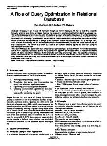
The query was executed 6 times with the optimizer being forced each time to use a different order of accessing the various tables, with the following results:

Table Order

Time Taken

te, m, tt

96 seconds

m, te, tt

22 seconds

tt, m, te

113 seconds

tt, te, m

110 seconds

m, tt, te

118 seconds

te, tt, m

107 seconds

Figure 1.1 – Execution times for various table access orders

The two sets of results that have been emphasized (bold and centre) are the best and worst case scenarios for this particular plan. It can be seen here that the difference between the two is substantial, with the worst case taking more than 5 times longer than the best case. It is for this reason that query optimization is so important, to ensure that the query optimizer chooses to execute the best plan, as opposed to the worst one.

The cost of each plan is evaluated by applying a cost model to the statistics about the execution environment that the Query Optimizer has access to. The cost model expresses cost as a function of the resources necessary to execute the query. These costs can be summarised as being attributable to the following;

Communication: This is the cost of transmitting data from the site where it is stored to the site where it is processed.

Secondary Storage: The cost of loading pages of data from secondary storage into main memory. This depends heavily on the size of the intermediate result sets in the execution, the clustering of data on physical pages, the size of the available buffers, and the read speed of the storage device.

Storage: The cost of occupying secondary storage space and main memory buffers over time.

Page 4 of 123


Molupe J. Mothepu

Computation: The cost of using CPU time, which is how CPU intensive the query is.

The communication cost is only a concern in distributed database systems where the Optimizer needs to access data that resides on disparate machines and needs to factor in the network latency. The storage cost is only considered if storage has become a system bottleneck and affects the execution, which is generally not the case. The two remaining contributors are the cost of computation and secondary storage access. Of these, the more generally significant one is the secondary storage access, with CPU cost only really becoming an issue with computationally intensive queries. Florescu et al. [1999] say it best by describing the process of query optimization as taking a query, which describes the data, and turning it into an execution plan that accesses the data where it is physically stored, and then applying a set of physical operators to it, eventually yielding a desired dataset.

The performance difference between the best and second best plan can be significant in time critical applications and the difference between the best and the worst plan can be substantial, making the choice of execution plan, a critical and delicate process.

1.3 – Chapter Summary

This chapter introduced the aim of this paper and gave a brief description of the significance of Query Optimization to the performance of database management systems, with specific focus on the data retrieval function. It also presented a high level view of the task of generic query optimization without going into too much detail on the inner workings of the actual process. The next chapter will give an indepth view of the process of query optimization and some different approaches to it.

Page 5 of 123


Molupe J. Mothepu

Chapter 2 – The Lit Review This chapter aims to give some insight into the conceptual aspect of query optimization and also present some of the work that has been done on the topic over the years. Query Optimization as a process is looked at in depth, in order to provide a foundation for the practical aspect of the process, which will be looked at in the chapters that follow.

The bulk of this Chapter is just to give some insight and background into the science of query optimization, but the focus of the paper lies in section 2.2 – The Query Optimization process, with specific focus on the choice of execution plan, and the factors in commercial database systems that influence the speed of this choice and its execution.

2.1 – Components of the Query Optimizer

According to Chaudhuri [1998] there are two components to the query evaluation system of a DBMS; the query optimizer and the query execution engine. The execution engine takes a plan supplied to it by the optimizer and executes it. This execution involves the implementation of a set of physical operators [Chaudhuri, 1998], which are actual implementations of relational algebraic expressions such as joins and sorts. The set of physical operators includes but is not limited to; external sort, sequential scan, index scan, loop join, and sort-merge join. The query optimizer takes as an input, a parsed representation of a query, generates a space of possible execution plans for it and then chooses the most efficient one. The execution engine basically takes at least one dataset as input, processes it, and produces an output dataset. Ioannidis [1996] on the other hand, describes four components of the optimization system, and breaks them down into more detail. A summary of them is as follows: •

The query parser: Checks the validity of a query and then translates it into a relational algebraic expression, or another equivalent internal representation.

•

The query optimizer: Evaluates all the algebraic expressions that are equivalent to the given query and chooses the one estimated to be cheapest. Page 6 of 123

Database Query Optimization •

Molupe J. Mothepu

The code generator or Interpreter: converts the plan chosen by the optimizer into calls to the query processor.

•

The query processor: executes calls from the code generator to retrieve data.

The focus of this paper is the one component that is common to both of the authors; the query optimizer.

Ioannidis [1996] goes on to break down the optimizer into six modules. In commercial implementations of the optimizer, not all the modules are included and some of them may be integrated but for completeness, a brief description of each is included: •

Rewriter: Applies transformations to the given query in the hope of producing more efficient but equivalent plans. Examples of these transformations are that nested queries can be flattened out and views replaced with their definitions.

•

Planner: Examines all possible execution plans for each equivalent representation produced by the rewriter and selects the one with the lowest cost. Inputs are obtained from the Algebraic Space and the Method-Structure Space, which are described below.

•

Algebraic space: Produces a series of actions, normally in an algebraic (relational) form as formulas or as a tree. These actions are the execution orders that are to be considered by the planner.

•

Method-Structure Space: Determines the implementation choices of the plans obtained by the algebraic space. This is dependent on the join types supported by the DBMS, the building of data structures and other such DBMS specific implementations. Complete execution plans are produced, complete with physical operator choices for the algebraic operators.

•

Cost Model: Specifies the arithmetic formulas used to estimate the cost of the execution plans.

•

Size-Distribution Estimator: Specifies how the sizes of relations, indices and query results are estimated. This component determines what statistics will be kept in the database catalogue.

Page 7 of 123


Molupe J. Mothepu

The main modules, that are also common to most optimizers, are the algebraic space, the planner, and the Size-distribution modules.

2.2 – The Query Optimization process

As stated in the first chapter, query optimization can be viewed as a difficult search problem. In order to solve this problem, the following are required: •

A search space: The space of all algebraically equivalent query execution plans.

•

A cost estimation model: Used by the enumeration algorithm to assign costs to each plan in the search space.

•

An enumeration algorithm: Examines the search space, assigns costs and chooses plan with lowest cost.

Ideally the search space should include low cost execution plans, the costing model should be accurate and the enumeration algorithm should be efficient [Chaudhuri]. Unfortunately, this ideal setting is not easy to achieve. At this stage it should be mentioned that all the literature concentrates on a specific type of query which is known as a Select-Project-Join query (also known as a conjunctive query, or a nonrecursive Horn clause [Ioannidis. 1996]). Each of the above problem requirements will now be discussed.

2.2.1 – The search space 2.2.1.1 – Representing the queries: Query Trees

This is what is referred to by [Ioannidis] as the algebraic space. It contains all the algebraically equivalent query execution plans. The number and nature of these plans is strongly related to the set of physical operators that the DBMS supports. Each of these plans can be represented in a number of ways but the most common way is that of a query tree in which a selection is denoted by σ, a projection by π and a join by . In such a tree, leaves are database relations and non-leaf nodes are the result of the application of the corresponding operator to the relations generated by its child nodes.

Page 8 of 123


Molupe J. Mothepu

Each result is sent up the tree through the edges which represent data flow, until they reach the root node which is the final result of the query. Select-Project-Join (SPJ) queries yield operator trees that are characterised by a linear sequence of the join operators in the query.

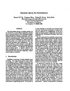
An example is provided for clarity. The query; select name, degree from student, degree where student.dgrCode = degree.dgrCode and age > 22

can be represented by the following query tree π

Name, floor

dgrCode = dgrCode

σ

Age > 22

degree

student

Figure 2.1 – Example Query Execution Tree

2.2.1.2 – Building the Search space

As was mentioned earlier, the algebraic space tends to be very large because of the commutative and associative properties of joins, and increases in size with an increase in query complexity. In many commercial implementations of optimizers, the search space is reduced by placing restrictions on the plans, effectively filtering out a portion of them. Ioannidis [1996] explains three different rules that are often used to achieve this restriction. The first rule basically states that selections should be processed as relations are accessed for the first time and projections are processed as results are generated. This results in a situation where all operations are dealt with as if they were Page 9 of 123


Molupe J. Mothepu

part of the join execution. Processing joins and selections in this manner is much cheaper in terms of time and resources than processing them separately, so any plan that does not fit this criterion is suboptimal by default.

Rule One does indeed prune the search space, but it by no means leaves it in a desirable state. Rule Two is often used to further reduce the number of plans. This rule states that relations will always be combined through the joins specified in the query. This ensures that cross products are never formed, unless they are explicitly requested of course. Cross products are formed as a result of joining relations that have not been specified as joined in the original query. The effectiveness of this rule comes from the fact that cross products tend to generate large sets of results. Some implementations go even further than these two rules and add a third rule to restrict the search space.

Rule Three’s restriction is that the inner operand of each join should be a relation and never an intermediate result. This restriction leaves only trees that are known as being left-deep as opposed to right-deep (trees that have their outer relation being a database relation as opposed to an intermediate) or bushy (trees that have at least one join between two intermediates). It is agreed upon by a lot of the authors that the third rule may well eliminate the optimal plan because bushy trees may result in a cheaper plan. In fact, Florescu et al [1999] stipulate that in the presence of limited access patterns, it can be shown that in certain cases, left deep trees will include only plans with Cartesian products, whereas there will exist a bushy tree that doesn’t. In this case, the space of bushy trees must be searched. The underlying theory of limited access patterns is beyond the scope of this paper. Ioannidis [1998] also states that it is in fact more efficient to optimize a search space that includes bushy trees as well as left-deep than the space that excludes bushy trees. Even in light of this fact, the bushy variety of trees tends to be excluded because keeping them tends to substantially increase the search space. Ioannidis [1996] states that there are claims that more often than not, the cost of the optimal left-deep tree does not surpass that of the optimal tree overall by any significant factor.

There are two main reasons for choosing to use left-deep trees. The first is that when database relations are used as the inner relation, the ability of the optimizer to use prePage 10 of 123


Molupe J. Mothepu

existing indices increases. The second reason is that using intermediates as the outer relation in the join allows sequences of nested loops to be executed in a pipelined fashion [Ioannidis, 1996]. The resulting combination of these reasons reduces the cost of join trees. As an aside, right deep trees facilitate the sequencing of hash joins in much the same way that left-deep trees facilitate the sequencing of nested loops. But apart from this, there is no real advantage to using right-deep trees over any of the others. This third rule brings us closer to what we want, which is a search space that consists of enough plans for it to contain the optimal plan, but that’s also small enough to keep the optimization effort from becoming a bottleneck.

2.2.2 – Enumerating the Search Space In most of the literature, the cost model is the part of the optimizer that assigns a cost estimate to any partial or complete plan. It is also responsible for the determination of the estimated size of the resultant dataset for each operator in the plan’s operator tree. Ioannidis [1996] goes into a little more detail and actually identifies the module called the Planner as the module that does such. The cost model specifies the formulas which should be used, and the size-distribution estimator does the output stream size estimation. The Planner uses information from these two modules to explore and evaluate the search space in search of the cheapest plan.

2.2.2.1 – Estimates and statistics The exploration of the search space is one of the main areas of interest and research in query optimization. There are a host of theories about the best methods to use and under what conditions they should be used. Query evaluation algorithms tend to depend heavily on heuristics [Jarke and Koch, 1984] and assume an accurate knowledge of run-time parameters [Cole and Graefe, 1994]. The runtime parameters that are implied in this statement consist of, but are not limited to selectivity and resource availability. To a large extent, the optimality of the plan is dependent on the knowledge of the values in the database, but unfortunately the exact values are not always available to the optimizer so it must estimate. This is the case even though statistics are kept about the structure of the database, as well as statistical information describing the values in it. These statistics are found in the database’s system

Page 11 of 123


Molupe J. Mothepu

catalogue (also known as the data dictionary). The problem is that these statistics tend to not be as up-to date as would be desired. Another issue that exists with the statistics is approximation errors. As the number of tables in a join increases, the errors multiply and can increase exponentially [Kabra and De Witt, 1998]. The resource availability mentioned has to do with the state of the system. Things such as the amount of available memory and the load on the system are subject to change for every execution of a query, and can even change mid-query. This is especially true for object-oriented databases, which allow users to define custom data-types, methods and operators [Kabra and De Witt, 1998]. Something that needs consideration when dealing with run-time parameters is that queries tend to be cached after execution. This is to avoid having to re-optimize them if the same or a similar query needs to be executed soon afterwards. Because these “system state” variable tend to change, the specific plan in the cache, may no longer be the optimal in light of the system’s new state.

2.2.2.2 - Cost assignment and pruning There are certain elements that need to be present for any form of evaluation to take place during the optimizer’s search through the algebraic space [Ioannidis, 1996]. These are: •

The set of statistics that are maintained in the data dictionary about relations and indexes. These include but are not limited to; the number of pages in each relation, the number of pages in each index and the number of distinct values in each column.

•

Formulas that will be used to estimate the selectivity of predicates and to give an estimate of the size of the resultant set for every operator in a query tree. The aim here is to generate intermediate relations that are as small as possible.

•

Formulas that estimate the CPU and I/O costs for every operator. These formulas must take into account the statistical information of their input data streams, existing access methods, and any ordering that exists on the data. The concept of interesting order will be discussed in more detail in the following section.

Page 12 of 123


Molupe J. Mothepu

At the end of the day, the job of the enumeration algorithm is to search through the algebraic space of alternative trees, assign a cost to each plan, pruning them as required and then choosing the best plan within the space. This is done by taking the formulas and rules found in the cost model and applying them to plans based on the values that are estimated by what Ioannidis [1996] refers to as the size-distribution estimator. What this essentially does is give an estimate of the sizes of the results of queries and sub-queries and the frequency distributions of their data. As was mentioned earlier, the statistics that the size-distributor uses are only estimates based on the values that are in the system’s data dictionary and can be inaccurate. It is for this and reasons such as the increased complexity of user requirements, and the trend towards object-relational systems, that even the best optimizers can experience degradation in performance by choosing a sub-optimal plan [Kabra and De Witt, 1998]. I think Chaudhuri [1998] says it well by stating that an optimizer is only as good as its cost estimates. Assigning costs to the components of a query plan works in the following manner: •

Statistics are obtained from the data dictionary about the data in question

•

The statistics are used in combination with an operator and it’s input streams to produce: o An estimate of the statistics of the output data stream o An estimate of the cost of executing this operation

The first step is carried out once at the beginning of optimization and the second step can be applied iteratively until all the operators in the query tree have been handled. Once the cost for each operator is obtained, the overall cost for the tree can be computed by summing up the cost of each operator. The statistical information required to carry this out is the number of tuples in a data stream and the number of physical pages that it spans, because this basically determines the cost of data scans, joins and memory requirements. Statistics on columns in the data stream are also required because they can be used to estimate the selectivity. A problem that exists though is that it can be proven [Chaudhuri, 1998] that the task of estimating distinct values is provably error prone, meaning that for any estimation scheme, there exists a database where the error is significant. Accurate cost estimation and the propagation Page 13 of 123


Molupe J. Mothepu

of statistical information through operators in a tree remains one of the most difficult optimization topics in query optimization. Recent optimizers are called extensible because they are built in such as way so as to be able to incorporate new physical operators in a modular manner (plug and play). To sum up the actual process of optimization, it can be said that optimization is the process whereby the query optimizer takes in a query as an input and outputs an execution plan. The inputs that go into the optimizer are; the logically pre-processed query (the query as a relational algebra expression), information about existing storage structures and access paths, and the cost model. As discussed earlier, the information about the storage structures and access paths are kept in the data dictionary. The optimizer must use these inputs to generate all alternative logical execution plans, which describe alternative sequences of operations and intermediate results that lead up to the result of the query. These plans must then be annotated with details of the physical representation of data, including sort orders, physical access paths and other statistical information. The cost model is then applied to these augmented plans and the cheapest one chosen [Jarke and Koch, 1984]. The System-R optimizer is the foundation for most commercial optimizers. Most of the enumeration strategies in the literature are based on extending or slightly altering the System-R optimizer. The enumeration algorithm found in it is characterised by two techniques that form the basis of query optimization today. These are dynamic programming and interesting orders [Ioannidis, 1996].

2.2.2.3 – Interesting Order In any database system, there are a number of join algorithms that can potentially be used, depending on factors such as the size of the input tables, the number of rows that match the join condition (selectivity), and the operations required by the rest of the query [Wikipedia, 2006]. A brief explanation of the more commonly occurring join types, as described by Wikipedia [2006] follows: •

Nested loops: For each tuple in the outer join relation, the entire inner relation is scanned and any tuples that match the join condition are retained. If either of the tables is very large, the efficiency of this algorithm drops substantially

Page 14 of 123


Molupe J. Mothepu

because it scans all tuples in all the tables. This can be highly efficient if the iteration is performed on indexes [Jarke and Koch, 1984]. •

Block loops: This is the same as the nested loop but it only scans the entire inner relations for each block in the outer relation, as opposed to for each tuple in the nested loop. This results in more computation for each tuple in the inner relation, but requires far less scans of it.

•

Hash-Join: A hash function is applied to the join attribute of the smaller relation, and a hash table is built. The larger table is then scanned and the relevant rows found by looking into the hash table. This is done by computing the same hash value on the hash key (join attribute) and checks for a match in the hash table. The advantage of this join is that it is only necessary to read each table once and no sorting is necessary. Ideally, the smaller relation should be able to fit into main memory.

•

Merge-Join: If both relations are sorted on the join attribute, then execution of this join is easy. For each tuple in the outer relation, the current group from the inner relation is scanned, and each tuple from the group that matches the join condition is retained. Once all relevant values in the group have been found, both the inner and outer scans can move onto the next group. A group consist of a set of contiguous tuples with the same value in the join attribute. If the primary key is the join value, then each group will have one member. If one or both of the tables are not sorted on the join attribute, then this needs to be remedied.

If both relations are sorted on the join attribute, then the Merge-Join is the most efficient. If one of the relations is very large and indexes are used, nested loops are preferred. For cases where one of the relations is small enough to fit into main memory, block loops or hash joins are favoured. Hash joins work best when there is a very large difference in the size of the relations. The efficiency of the Merge-Join is one of the reasons why we’re interested in the order or the relation that results from a join. An Interesting order is existent when having the result of one join sorted on a particular attribute will reduce the cost of a subsequent join. This means that there exists a situation where, if the order in which relations (including intermediates) are

Page 15 of 123


Molupe J. Mothepu

accessed is ignored, the globally optimal plan will be missed. As a result of this, when dynamically pruning query trees, two trees will only be compared if they are representative of the same expression and have the same interesting order. It is thus possible for a plan to be more expensive at some point but yield a result that will take away the need to sort, facilitating the use of a Merge-Join at a later stage.

2.2.2.4 – Dynamic programming The dynamic programming algorithm is a dynamically pruning exhaustive search algorithm. It is based on the assumption that the cost model adheres to the principle of optimality which states that “the components of a globally optimal solution are themselves globally optimal” [National Institute of Standards and Technology, 2004]. This basically means that all the decisions made en route to the optimal decision are themselves optimal. It therefore follows that to find the optimal solution of a query consisting of n joins, only the optimal plans for sub-expressions of the query that consist of n-1 joins need to be considered and then extended with an additional join. An SPJ query is viewed as a set of relations to be joined and the trees are created by inspecting the number of relations that have been joined so far while pruning trees that are known to be suboptimal. A nice example of this given by Ioannidis [1996] is that the optimal plan for a query with a set of join relations {R1, R2, R3, R4} is a result of picking the cheapest plan from the optimal plans of joining the relations in the following orders: Join ({R1, R2, R3}, R4) | Join ({R1, R2, R4}, R3) | Join ({R1, R3, R4}, R2) | Join ({R2, R3, R4}, R1)

It is assumed that the result of the 3-relation (whichever combination) join is the optimal one and is being extended by joining that result to the last relation. All other plans can be ignored. It therefore follows that dynamic programming takes a bottom up approach, increasing the number of relations joined as it goes up the tree until eventually all that is left is a pool of trees that are the most optimal in the group of trees with similar join sequences, and then choosing the most optimal from among them. So basically, only the optimal plan from each group is chosen and then only the most optimal plan from this set of optimal plans is chosen as the global optimal. It can afford to be exhaustive because it prunes sub-optimal trees along the way, it does not need to fully evaluate the next plan if at any point it proves to be less optimal than the

Page 16 of 123


Molupe J. Mothepu

last one evaluated. It in fact uses a pilot pass, whereby a complete plan is computed and then all sub-plans that are more expensive than that particular one are discarded [Reddy and Haritsa, 2005]. Care must be taken when pruning trees which may at first appear to be suboptimal because of the concept of the interesting order. Dynamic algorithms exist to counter the production of “static” plans, which as was mentioned earlier, tend to assume accurate knowledge of the run-time parameters during optimization. The idea is for the optimization to “react” to the actual values of run-time parameters as the query is being optimized [Chaudhuri, 1998]. The problem that arises from this is that memory requirements and running time increases exponentially with the number of joins [Ioannidis, 1998]. It is said by [Cole and Graefe, 1994] that the additional overhead is shadowed by the advantages of using this type of algorithm. Advantages include that they are as robust as brute force runtime optimizers. Robustness in this instance means that they retain their optimality even when parameters change between compile time and run-time. The algorithm is therefore superior to the static plans generated by compile-time optimization and algorithms which implement full run-time optimization, which tend to have much more overhead. Cole and Graefe [1994] suggest achieving a balance by doing the bulk of the optimization at compile-time and then holding off some decisions until runtime. This is achieved by using a choose-plan operator which postpones the choice between two or more plans until start-up time, when the actual values of required parameters become known. Through time though, there have been a number of alternatives to the dynamic programming approach. An example is Viglas and Norton’s [200] rate-based as opposed to cost-based optimization that is used for streaming information sources. The claim is that their algorithm takes a constant time to find the first viable solution with an increased search space, as opposed to traditional dynamic programming, which as we discussed earlier, degrades with the number of relations involved in the join. Even though there are more efficient algorithms out there, it is important to have knowledge of dynamic programming because it is the yardstick to which all other algorithms are compared [Florescu at al., 1999], and because it is the most widely used in most commercial database systems [Ioannidis, 1996].

Page 17 of 123


Molupe J. Mothepu

2.3 - Types of Optimization Although the focus of this paper is on cost-based optimization because it is the most widely used type, it is worth giving the other existing types a brief mention.

2.3.1 - Rule-based optimisation This type of optimization has been phased out because of its inefficiency. The optimizer chooses the best plan based on a set of syntactical rules and rankings of the various access paths. Statistical information is ignored. Certain types of access paths take precedence over others in certain situations, regardless of the context of execution. This means that suboptimal choices may be chosen because of the rigidity of the rules.

2.3.2 - Semantic Query Optimization This has to do with using integrity constraints defined in the database to rewrite one query into semantically equivalent ones [Ioannidis, 1996]. This is not the same as just using transformations to rewrite a query into an algebraically equivalent one. In semantic optimization, the query is turned into another query, which means the same thing but is going to be easier to optimize (for example, one that uses indexes, if the original one did not). The semantically equivalent queries are then optimized in the regular manner and the most efficient plan found is retained. Heurist must be used with this type of optimization to establish rules on when it would be beneficial to rewrite a query in this manner and when it should be left in its original form.

2.3.3 - Global Query Optimization There often arises the need to run and/or optimize more than one query at a time, whether it is because of the presence of a union, concurrent requests from users or queries requested by an application. In this case it is better to have a globally optimal plan. This plan may be suboptimal for each individual query but is optimal for their execution as a group [Ioannidis, 1996]. The existing storage structures and access paths in a database system can not be optimized for a single query, but can be Page 18 of 123


Molupe J. Mothepu

optimized globally, for all plans [Jarke and Koch, 1984]. This particular topic is the focus of multiple query optimizers.

2.3.4 - Parametric/Dynamic Query Optimization This particular type deals with embedded queries, which are optimized once at compile time and use the same execution plan each time they are run at run-time. Parameter values may change significantly in the time between compile time and runtime and a plan which was optimal at compile time can be severely sub-optimal at run-time. There are a number of ways of combating this. As was mentioned earlier, Cole and Graefe [1994] suggest putting off some decisions until run-time, where there is a more accurate knowledge of parameter values. Kabra and De Witt [1998] in turn put forward the idea of dynamically monitoring the changes in estimated and actual parameter values and changing (re-optimizing) the execution plan during run-time, according to the actual values. Another technique is to optimize queries at compile time in a brute-force manner, whereby all possible values of crucial parameters are taken into account when building the search space. At run-time, the plan which matches the actual parameters is chosen. This method has little overhead at run-time as the bulk of the work is done at compile time [Ioannidis, 1996]. The next section deals with some implementations of commercial optimizers.

2.4 – Chapter Summary The aim of this chapter was to provide some foundation for understanding the inner workings of the query optimization process. This provides some preparation for the ensuing discussions. These discussions are based on the analysis of query optimizer performance in the commercial database systems. The next Chapter gives a description of the design of the evaluation that forms the basis of this paper.

Page 19 of 123


Molupe J. Mothepu

Chapter 3 – Design This Chapter aims to provide a description and explanation of the design choices made and considerations taken, in the evaluation process. It will explain which platforms were used, which database management systems were used, and give a brief explanation of why each was selected. A description of the test bed will also be included, which will encompass the structure of the database used for testing and the choice of test variables.

3.1 – Platforms

Two platforms were used in this evaluation. These platforms are Microsoft Windows Server 2003 and Ubuntu Linux 6.06 Dapper. Both of these platforms were run on the same machine, using a dual booting configuration, to ensure that each is operating on the same hardware platform. The hardware specifications of the machine that these operating systems run on are as follows:

Dual 3.40 GHz Intel(R) Pentium(R) 4 CPU

3.5 GB RAM

2 x 112 GB SCSI Hard Disks (1 HDD per operating system)

A brief explanation of the reasons for choosing each of the operating and database management systems ensues.

3.1.1 – Windows Server 2003

Windows Server 2003 was chosen because it is the current recommended server operating system by Microsoft. Windows Server 2000 was a very prolific operating system and Server 2003 has promised to be even more powerful and robust than its predecessor [Microsoft, 2006]. Windows owns a large share of the server operating system market [Shankland, 2006], and most of the users of Server 2000 will eventually migrate to Server 2003 and so it was a logical choice to choose this as a platform. Service Pack 1 was also installed to bring the operating system up-to-date. Service Pack 2 is still in its Beta stage and so was not installed for stability reasons, in

Page 20 of 123


Molupe J. Mothepu

that it might cause unexpected behaviour.

3.1.2 – Ubuntu Server Dapper

Ubuntu Linux was the second operating system of choice. This choice was largely due to the fact that one of the database management systems chosen for the evaluation is open source. Ubuntu was chosen specifically because of the wide support that exists for it, its ease of use, and availability. Another reason is that Ubuntu is growing in popularity in South Africa because of it being developed in South Africa [Ubuntu website, 2006]. It was therefore found to be a relevant test bed in the South African context. The version that was used is the most recent distribution, which is 6.06 Dapper. It was installed as a server, which is a much more compact installation than the desktop installation, and does not come with a GUI. The Secure Shell Daemon (sshd) runs on the server, enabling remote access via PuTTy or any other ssh1 client.

3.2 – Database Management Systems

3.2.1 – SQL Server 2005

Like the Windows Operating system, Microsoft's SQL Server enjoys a large share of the industry in its use as a database management system [Pettey, 2005]. SQL Server 2000 was a large success and SQL Server 2005 builds on the strengths that SQL Server 2000 brought forward. SQL Server 2005 with service pack 1 was installed, which as of the writing of this paper was the most recent update.

The choice for this was based on the popularity of this product, coupled with its availability and impressive amount of documentation and support that it has. It also sports a rich set of tools that can be used to monitor the database server's performance and the queries in particular. Being one of Microsoft's “golden products”, SQL Server is one product that Microsoft put a lot of effort into, and it has been known to pay off. It is the DBMS of choice to a wide range of companies, providing an easy to use, 1

ssh stands for Secure Shell and is a means of securely accessing a remote machine via a command line interface, or “shell”.

Page 21 of 123


Molupe J. Mothepu

readily configured database solution. It has proven itself robust, reliable and efficient in data retrieval, as well as sporting much support for programming constructs. SQL Server 2005 is supposed to be the most programmer friendly database system that Microsoft has released to date [Microsoft, 2006].

The above reasons are why SQL Server was chosen for this query analysis evaluation. Next is a brief description of the second DBMS that was chosen for the evaluation.

3.2.2 – MySQL 5.0.22

MySQL is an open source database management system which has gained great popularity over the years [MySQL, 2006]. Because of the nature of open source software, there are many versions or releases of MySQL, each attempting to address the weaknesses identified in the last. As of the time of the writing of this paper, the most current version was version 5.0.22. MySQL is very well documented and has a vast community of users and developers globally who contribute with bug reports and fixes, which adds greatly to its support. It is the most widely used open source database management system, rivalled only by PostgreSQL and Firefox [Sullivan, 2005]. One of the aims of this project is to compare the performance of proprietary and open source database systems, so it came down to a choice between the two biggest players in the open source database world, which are those mentioned above.

There have been many debates, which are beyond the scope of this paper, as to which of the two rival open source databases, MySQL and PostgreSQL are “better”, and still, like in most debates, there is no clear cut answer. MySQL is more widely used and so support for it in the application world is wider than for PostgreSQL, and the larger community of developers that MySQL sports means that technical support for it is also greater. Both systems are able to handle high volumes and both perform well in terms of speed, but it has been said that MySQL's MyISAM tables are more lightweight and hence faster than PostgreSQL's [Gilfillan, 2003].

It is for the speed, compactness, ease of access to support, and market share, that MySQL was the choice as the second database system. The next section gives a brief

Page 22 of 123


Molupe J. Mothepu

description of the tables in the database that was used as the test bed.

3.3 – Overview of the database

The database is currently made up of 14 tables which have the following cardinality:

Table Name

Cardinality

consumer

53 990

consumer_classification

4

consumer_details

39 352

consumer_connections

60566

meter

58 370

meter_connections

70 427

payment_method

9

poc

55 898

poc_details

41 658

token

2 374 388

transaction_entry

2 352 035

transaction_financial_item

7 051 139

transaction_item_type

115

transaction_type

7

Figure 3.1 – Names and cardinalities of the tables in the test database

For a more accurate description of the column names, data-types and relationships between tables, refer to Appendix A. This appendix provides the T-SQL statements that generated the tables and indexes in SQL Server. It should suffice at this time to mention that each table is indexed on at least the primary key.

It is worth noting that MySQL has two main database storage engines; InnoDB and

Page 23 of 123


Molupe J. Mothepu

MyISAM. The difference is that InnoDB is transactional and MyISAM is not. MyISAM is claimed to be much faster than InnoDB but SQL Server tables are transactional so the InnoDB tables would be the fairest comparison with the SQL Server tables. Though this is the case, MyISAM is the default storage engine, and the one recommended on a general basis, it will be the engine of choice for the MySQL testing.

The next section outlines the choice in variables that will be tested for the evaluation.

3.4 – Identifying test variables

The focus of this paper was the effect of various factors on the performance of the Query Optimizers in terms of query execution time. A number of these factors were identified and a brief discussion of each is presented. These are the factors that were variables in the testing phase of the project.

3.4.1 – System variables

These are the variables that determine the query execution environment. These variables generally encompass items such as the caches available, the buffers available, and any other server parameter that is documented to have an effect on the speed of query execution in the database system. Each DBMS that was chosen enables the administrator to have access to, and modify the values for a number of server parameters. SQL server provides the sp_configure command and MySQL has the set command. Both DBMSes store the parameters in tables. In SQL Server, a normal select query on the sys.configurations table will display the parameters, and in MySQL they can be viewed by using the show [variables | status] command. There are a large number of parameters that are configurable, and only a handful that will directly affect the speed of query execution. The reasons for the choice of toggling server variables for optimality are presented next.

One of the reasons for choosing to tackle the optimization effort by focusing on the environmental variables is that optimizing the query run-time environment will have

Page 24 of 123


Molupe J. Mothepu

the effect of optimizing every query. This is contrary to the task of finding optimal ways for writing SQL statements, which would be very much dependant on the nature of the data required. It is a method of globally increasing the speed of query execution. Another reason is that it takes the task of query optimization out of the hands of the writer. By this it is meant that the writer of a particular statement needs to concern themselves less on building optimality into the statement because the server will be configured for global optimality. Another reason is that it is of interest to venture into whether or not the default settings used in the database systems are also the most optimal ones, that is to say, if the servers are configured for optimality straight out of the box. whatis.com [1999] states that a default setting is a setting that is used by a program when no user specified value has been given. It is predefined as a value that represents the value that most users would be likely to choose, not necessarily the optimal value.

The key variables for each server have been identified and will be presented in Chapter 4 - Methodology.

3.4.2 – Complexity of queries

Complexity in this context will be defined in terms of the number of joins. The aim with this is to check how the various database systems handle various levels of complexity in queries. The effect of the complexity on the choice of query execution plan will also be analysed. This stems from the fact that a complex query can often be written in a simplified manner, or vice versa, and it is of interest to view the effect that the complexity will have on the choice of execution plan.

3.4.3 – Size of the result set

Investigation will be carried out to determine whether the size of the final result set has an impact on the execution of the query. It is documented that the sizes of the intermediate datasets generated during query execution have a large impact on the choice of physical operator and thus execution plan. The result set for all execution plans, should be identical, but it is of interest to see whether having a query that

Page 25 of 123


Molupe J. Mothepu

accesses the same tables, using the same join predicates but requiring fewer records from the table, will have an impact on the execution plan, as opposed to the time of execution, which it will definitely have an impact on.

3.5 – Chapter Summary This chapter provided some insight into the design considerations for the evaluation. It was presented that the main reasons for choosing the various platforms were popularity, support and documentation, and performance debates between their supporters. The reasons for choosing server configuration as a goal were also presented. The next Chapter will provide details of the implementation of the evaluation.

Page 26 of 123


Molupe J. Mothepu

Chapter 4 – Methodology The process that was used to carry out the evaluation for this paper uses a “standard” scientific approach. By this it is meant that it was observation based. For the comparison section, the same query was run on both database servers and the execution plan and time were observed, documented, and compared. For the actual server optimization part, a number of variables identified as key to each DBMS were altered and the effects of this observed and documented. To reiterate, the aim of the server optimization (objective two of the project) is to identify those variables that cause a performance increase within the database server, with the goal of finding the best configuration. A more in-depth description of each testing process ensues.

4.1 – Objective One: The comparison

The process for running the tests for this objective took the following form:

For each DBMS For each query Get Execution Plan Run Query and record result Compare results for DBMSes

For the comparison between the two database servers, SQL Server was tested on Microsoft Server 2003, its native operating system and MySQL was tested on both Windows Server 2003 and Ubuntu Server. In SQL Server the queries were run via the SQL Server Management Studio, which provides a Graphical User Interface much like the Query Analyzer in SQL Server 2000. With MySQL the queries were entered via the command line and using the MySQL Query Browser. Both Database Servers were tested using their default installations, and the same queries were run on each, using standard ANSI SQL statements. For the first set of the tests, the buffers and cache were cleared before each execution, so as to force the optimizer to re-evaluate the query from scratch, each time it was run. It was also done to ensure that similar queries did not have their plans or speed of execution influenced by the cache. This Page 27 of 123


Molupe J. Mothepu

was just to test each database system’s ability to handle queries that it executes for the first time. It must be emphasised though, that in a production environment, this clearing of buffers and cache is not only unusual but undesirable, as this takes away the advantage of having a cache, which is to have frequently used data, readily accessible. A similar timing test was carried out using the same queries, without clearing the buffers. Each server only had the single connection that was used to carry out the testing open, so the environment was single-user, although it had been setup as multi-user on both servers. Fourteen queries which vary in the number of joins run on each server.

4.2 – Objective Two: Server Optimization for queries

For this section, the focus was more on the individual performance of each database Server. The literature on both servers was searched in an endeavour to identify those variables that are critical to the performance of each server. These claims were then tested by evaluating the actual effect of changing the said variables on the query execution times. For each server, two queries would be tested for each variable, one that runs below one minute and one that runs for longer than one minute. The process followed for each of the queries is as follows:

For each DBMS Identify server variables which are potentially relevant For each query For each variable For each value between min and max values for variable Get Execution Plan Run Query and record result Increment value of variable by chosen increment factor Tabulate and identify optimal values per variable

After this process has been carried out for each variable, the optimal value of each variable will be known. The next section provides a description of each of the variables that were claimed by experts in the various database systems to be of most

Page 28 of 123


Molupe J. Mothepu

relevance to the speed of execution.

4.2.1 – SQL Server System Variables

All the server system variables in SQL Server are stored in the sys.configurations table, which can be queried like any other table, to display their values. This table has 9 columns which are; configuration_id, name, value, minimum, maximum, value_in_use, description, is_dynamic, and is_advanced. It has a cardinality of 62 and belongs to the master database. The sp_configure command is used to change any of the values of the records in this table. Some of the variables need a server restart to take effect, but most of them take immediate effect. Of the 62 possible variables, the following were identified and tested for their effect on query execution:

Variable

Description

min memory per query

This is the minimum amount of memory in kilobytes that will be allocated to each query for execution. The query is entitled to at least this much.

query governor cost limit

The upper limit for the time period in seconds for which a query may run before being abandoned. If a query looks like it will run for longer than this, it will not be allowed to execute.

cost threshold for parallelism The upper limit for the time period in seconds for which a query is estimated to run before SQL server creates and runs parallel plans. Shorter queries will run serial plans and longer ones will run parallel plans. This is only valid in the presence of multiple processors. Max degree of parallelism

The maximum number of processors on the machine that can be used for processing a query.

Figure 4.1 – Variables identified as key to query execution in SQL Server 2005

Page 29 of 123


Molupe J. Mothepu

Some relevant information for the above variables at default is as follows:

Variable Name

Value

Minimum

Maximum

Value_in_use

cost threshold for parallelism

5

0

32767

5

min memory per query (KB)

1024

512

2147483647 1024

query governor cost limit

0

0

2147483647 0

Max degree or parallelism

0

0

0

Figure 4.2 – Default, minimum, and maximum values for variables identified in Figure 4.1

The difference between value and value_in_use is that for variables that require a server restart, the value column, will hold the value of the variable as it will be at the next restart. For dynamic variables (which do not require a restart) the two columns will always hold the same value after running the reconfigure or reconfigure with override command, the latter enabling a rollback if the changes cause any instability in the server.

It is worth mentioning that the amounts of memory specified in min server memory and min memory per query will only be reserved once SQL Server has found an instance where it requires the amount specified. If it never actually needs these amounts, it will never actually reserve them, and will run on less memory. It must also be stated that in all the literature encountered, changing any of the variables in the sys.configurations table was advised against. This is due to the fact that SQL Server is supposed to dynamically optimize itself for query execution. It is for this reason why there is so little control offered over the execution environment, as revealed by the small number of configurable variables overall, and especially ones that deal specifically with query execution.

4.2.2 – MySQL System Variables

The server variables in MySQL can be accessed via the show variables command. This command gives a tabular representation of all the variables and their values. Unlike the sys.configurations table in SQL Server, which has a large number of

Page 30 of 123


Molupe J. Mothepu

columns, the table resulting from the show variable command has only two fields, Variable Name and Value. This resultant table has a cardinality of 216 tuples when MySQL is on Ubuntu and 211 tuples when in Windows.

Like in SQL Server, some of these variables are dynamic, meaning that their values can be changed while the server is running, and some of them require a server restart. Apart from dividing them by this characteristic, there are global variables and session variables. There are those variables that are only global or only session but a lot of the variables are both global and session, which means that the value can be altered for the session or globally. Variables that are global will only affect new connections to the system, whereas session variables affect connections that are currently in place.

The variables identified by experts as being relevant in MySQL can, for the most part, be separated into two groups. These groups are the caches and the buffers. Caches are shared between all threads and are allocated once whereas buffers are not shared and are allocated to each thread on demand. The ones that are of interest in this case are the buffers. As was said earlier, the cache will have some effect on the speed of execution by virtue of being cache (the purpose of cache being to store frequently / recently accessed data for faster access on subsequent calls), and so of most interest is the effect of changing the values of the various buffers. A few variables that are neither caches nor buffers have also been identified as being interesting. A summary of all the variables is given in the figure below:

Page 31 of 123


Molupe J. Mothepu

Variable

Description

join_buffer_size

Size of the buffer for joins that do not use indexes i.e. which do full table scans.

net_buffer_length

Minimum size for the connection and result buffer

optimizer_prune_level

Controls the heuristics applied while pruning less attractive execution plans during optimization.

optimizer_search_depth

The maximum depth of the search. More depth results in a more optimal plan, but found slower. Less depth results in a quick find of a sub-optimal plan.

key_buffer_size

Controls the size of the key cache (which caches the most frequently used indexes).

table_cache

Number of tables that MySQL can accommodate in cache. This is per thread, not global.

Figure 4.3 – Variables identified as key to query execution in MySQL

The values at default for the above variables are as follows;

Name

Default Value Windows

Linux

join_buffer_size

131072

131072

net_buffer_length

16384

16384

optimizer_prune_level

1

1

optimizer_search_depth

62

62

key_buffer_size

333447168

16777216

table_cache

256

64

Figure 4.4 – Default values for key variables identified in Figure 4.3

The global variables will not have any effect on any sessions that were open before the change and so would require a server restart to become globally applicable. It was

Page 32 of 123


Molupe J. Mothepu

found that the easiest way to carry out the tests was to change the values in my.cnf file which allows user specified values to be used at server start-up, and then restart the server with the new values.

4.2.3 – Overview of the queries used.

The queries in the testing differed mainly in terms of the number of joins and size of the resultant set. For the comparative test, all the queries were run on both the database systems. For the server optimization tests, only a select few of the 14 queries were used. Results for all the queries will not be included in this test due to time constraints, especially with some of the queries taking several minutes to run. A full description of the queries is presented with the results of their executions in Chapter 5.

4.3 – Chapter Summary

This chapter provided some insight into the methodology used for the various tests that were carried out. It also presented the specific variables of interest in the various database systems. The next chapter presents the results for the tests.

Page 33 of 123


Molupe J. Mothepu

Chapter 5 – Results The following section will give the results that were obtained for the testing carried out for each project objective. The first section will detail the results of the comparison of the ability of the two database systems to execute various queries in a timely fashion. The second section will then present the results of the tests that were run in the attempt to optimize the environment that the queries run in, by identifying optimal values for each server setting that has been identified as key to query execution.

5.1 – Objective One: The Comparison

This section will describe the results of how fast each database system could execute a series of increasingly large queries. It is reiterated that both systems are working on a default configuration, with no system variables having been altered. A series of queries was run on each system, and the time to execute, along with the query execution plan were analyzed. The format that this section will take is that a brief introduction into the join types that were encountered for each database server will be given, along with the tools that were found useful in the evaluation. After this, each query will be introduced, followed by the time the various servers took to execute it, in both tabular and graphical format. The execution plan will then be analysed.

5.1.1 - Analysis of MySQL

This section provides some insight into how MySQL query execution was analysed. First a description of the types of joins that were encountered in the tests will be given, and then a description of how the query trees were then built from the information that MySQL supplies about query execution.

5.1.1.1 - MySQL Joins

According to the manual, MySQL uses what is known as single-sweep multi-join method. This means that it accesses the first table, then finds a matching row in the Page 34 of 123


Molupe J. Mothepu

second table, then in the third, and so on, until the a row in the last table has been found, whereby it starts again. To illustrate, if there are 4 tables, R1, R2, R3, and R4, they are joined in the following manner (((R1

R2)

R3)

R4) but on a row-

by-row basis.

There are a number of ways that MySQL accesses the data in a table to perform joins, but those that were seen in the testing for this project are the following: •

All - According to the MySQL manual, this is the worst type of join because it implies that a full table scan will be performed on the table for each combination of rows from the table or intermediate result that is being joined to.

•

Ref – Similar to the All in theory except that only the values with matching index values are read for each combination. This implies that the key (join attribute(s)) that is used does not uniquely identify each row in the table, but still does not match too many of them.

•

Eq_ref – A refinement of the ref type, whereby only one row is read in this table for each combination of rows in the previous ones. Here, the key used will be a primary key or unique index.

5.1.1.2 - MySQL Query Analysis Tools

MySQL provides a command that takes the form explain where is the actual query itself, without angular brackets. This command is immensely useful as a query analysis tool. Its output is the query execution plan, in tabular form, for the specified query. MySQL does not actually execute the query but rather just lists the tables in the order in which they will be accessed, along with some other useful information.

The fields that are of most interest are:

select_type: The type of select it is, for this particular table. Example values are simple, union, and sub-query.

Page 35 of 123


Molupe J. Mothepu

Table: The name (or alias) of the table. Type: The type of join performed on the table, with the last table or with the result of the last join. Example values are system, const, and eq_ref. Rows: The number of rows that MySQL thinks it will have to examine to execute the query. Extra: Any additional information goes here. Example values are; Using Index, and Using where. These are the two that can be seen in the results from the explain commands that were run for this project. The using where means that the rows in the table were restricted based on some condition. The using Index means that column information from the table is retrieved completely by using information from the index tree, and not actually doing any disk seeks to read the row.

So in the example below:

Figure 5.1 – Example output from an explain command at the MySQL command line

It can be seen that in order to execute the query we need to do a full table scan of the consumer table (referred to in the figure above as c, in the table column) and has to look at an estimated 53 990 rows from it. An eq_ref is carried out on the consumer_details table (referred to as cd) to join each row in the consumer table, using the primary key as the join attribute, and an estimated 1 row will be accessed from this table for each row in the consumer table. The consumer_connections (referred to as cc) table is then accessed using a ref type join and using the where clause, as can be seen in the Extra column. It can also be seen that only one row from this table is expected to be returned for each row in the intermediate data stream that results from joining the previous two tables. This output, in conjunction with our

Page 36 of 123


Molupe J. Mothepu

knowledge of the way MySQL performs joins allows us to build the following execution plan for the query:

Select consumer_surname, consumer_first_names, consumer_active, consumer_connect_date from consumer c, consumer_details cd, consumer_connections cc where c.consumer_id = cd.consumer_id and c.consumer_unit = cd.consumer_unit and c.consumer_id = cc.consumer_id and c.consumer_unit = cc.consumer_unit

Figure 5.2 – Execution plan derived from the explain command

The time taken for the query to execute is also provided after the results for the query have been provided, along with the number of tuples returned as follows:

Figure 5.3 – Example output from a query. Focus is on the execution time, which has been circled in MySQL

The number of reads that the query required can also be obtained from MySQL by using the show status command, which gives a tabular representation of the status of a number of system variables, which exhibit the system’s state. The variables that are of interest in this scenario are the key_read_requests which are the number of requests to read a key block from memory, and key_reads which are the actual number of

Page 37 of 123


Molupe J. Mothepu

physical reads of a key block from disk. The last_query_cost is also an interesting variable as it shows how much the calculated cost of the last query executed is.

5.1.2 - Analysis of SQL Server

This section is the equivalent of the previous one for MySQL. It describes how the SQL Server query execution was analysed. The type of joins encountered in the evaluation will first be presented, followed by the tools that were used in the analysis.

5.1.2.1 – SQL Server Joins

SQL Server uses a different method of joining from MySQL. The two types that were seen in evaluation are the Merge Join and the Hash Match. These are implemented in the manner that was mentioned in Section 2.2.2.3 – Interesting order. All the rows in the tables were accessed using a clustered index scan to read them. A clustered index is an index that is based on the same key that the data is ordered on, in effect ordering the indexes in the same order as the data in the table.

5.1.2.2 - SQL Server Query Analysis Tools

SQL Server provides the option to show a graphical representation of the query execution plan instead of executing the query. Alternatively, the option exists to actually execute the query and have the execution plan included in the output. It augments this by providing information including but not limited to the physical operator that will be implemented, the number of rows estimated, and the estimated I/O cost, in the form of a screen tips. The option that allows this is shown in figure 5.4 on the following page.

Page 38 of 123


Molupe J. Mothepu

Figure 5.4 – Screenshot of SQL Server Management Studio. Focus is on the option to “Display Estimated Execution Plan”.

And a sample output from having this option on, is as follows:

Figure 5.5 – Screenshot of the output of choosing to display the executed query plan instead of running the query.

A closer look at the query execution plan section reveals the true power of the tool, which is the descriptive screen-tips, an example of which can be seen in the figure on the following page.

Page 39 of 123


Molupe J. Mothepu

Figure 5.6 – Screenshot after having zoomed in on the execution plan. Focus is on the screen tip for the Hash Match join.

The above shows that the physical operation is a Hash Match and that the logical operation is an Inner Join. It also displays the estimated I/0 cost, which in this case is 0 (because I/O cost is assigned to the table scans, not the operators) and the CPU cost. The sum of the I/O and CPU cost are then given as the cost of the operator. The total cost of the query can be gained from placing the mouse over the select icon, which is the left-most item in the tree, which displays a screen tip. The cost of the sub-trees is also given, and the estimated number of rows that the join will yield. The size, in bytes, of each row is estimated. This tool gives an already graphical representation of the execution tree and therefore there is no need to build it.

SQL Server also has a facility to show the actual value of the number of reads required by the query. This value can be seen in the trace produced by the Server Profiler, as in below.

Page 40 of 123


Molupe J. Mothepu

Figure 5.7 – Screenshot from the SQL Server Profiler. Focus is on the number of reads, which is circled.

The columns of interest here are TextData, which provides an indication of the event that occurred, the CPU, Reads, Writes, StartTme, and EndTime. These are the variables which are useful in following the performance of the query. The time taken to execute each query was derived by subtracting the query StartTime from the EndTime, as in the columns in figure 5.7 above.

5.1.3 – Comparison Results This section details the results that were obtained in the comparison of the two database servers. The testing process is as outlined in Chapter 4. This section will present for each query tested; a description of the query run, the time taken to execute in tabular format, the time taken to execute in graphical format, and a graphical representation of the execution plan proposed by the server, and brief discussion of the results. For ease of reading, each query will be treated as a sub-section in its own right.

5.1.3.1 – Query 1

Query 1 is a simple select query that involves one table and no join operations at all. The results for this query are presented in the figure on the next page.

Page 41 of 123


Molupe J. Mothepu

Query 1 AS select * from consumer_details – 39 352 tuples SQL Server 2005

Windows MySQL

Ubuntu MySQL

1.64

0.21

0.21

Figure 5.8 – Query description and Execution times for Query 1

Execution Times for Query 1

1.64 1.80 1.60

Time in seconds

1.40 1.20 1.00 0.80 0.60

0.21

0.21 0.40 0.20 0.00 Yukon

W MySQL

UMySQL

Figure 5.9 – Graphical representation of Query 1 execution times.

For this test, SQL Server was much slower than MySQL by a factor of nearly 8, which performed equally well on each of the platforms that it was run on. The Query execution plans for the two systems are presented below. It should be noted that in this case, as in all other cases, the execution plans for MySQL were identical for both platforms.

Figure 5.10 – Execution Plan for Query 1

Page 42 of 123


Molupe J. Mothepu

For this particular query, the execution plan for all the servers was identical as there is only one table and no join, therefore the various execution plan can only differ in the method used to access the data in this table. SQL Server uses a clustered index scan whereas MySQL uses an ALL (full table scan) to access the data in the table. It appears that in this case, it was better to do a full table scan than to use indexes.

5.1.3.2 – Query 2

Query 2 is a single join between two tables consumer, which contains 53990 records and consumer_details which contains 39 352. The results are as follows:

Query 2 AS select consumer_surname, consumer_first_names, consumer_active from consumer_details cd, consumer c where c.consumer_id = cd.consumer_id and c.consumer_unit = cd.consumer_unit – 39 352 tuples SQL Server 2005

Windows MySQL

Ubuntu MySQL

1.20

0.66

0.21


Page 43 of 123


Molupe J. Mothepu

Query 2 Execution Times 1.20 1.20

Time in seconds

1.00

0.66

0.80

0.60

0.21

0.40

0.20

0.00 Yukon

W MySQL

UMySQL

Figure 5.12 – Graphical representation of Query 2 execution times

Once again, MySQL outperforms SQL Server, although it slows down on windows. An interesting observation is that MySQL on windows is the only server to have slowed down between this query and the first one. MySQL on Ubuntu stayed the same, and SQL Server actually sped up. The Query trees for this plan are as follows:

SQL Server 2005

MySQL


Page 44 of 123


Molupe J. Mothepu

These execution plans are once again identical. The only visible difference is the fact that SQL Server used a merge join, whereas MySQL used an eq_ref type join.

5.1.3.3 – Query 3

Query 3 builds on Query 2 with the addition of another table, consumer_connections which has a cardinality of 60 566 records. The result is as follows:

Query 3 AS Select consumer_surname, consumer_first_names, consumer_active, consumer_connect_date consumer_connections

from cc

consumer

where

c,

c.consumer_id

consumer_details =

cd.consumer_id

cd, and

c.consumer_unit = cd.consumer_unit and c.consumer_id = cc.consumer_id and c.consumer_unit = cc.consumer_unit– 45 476 tuples SQL Server 2005

Windows MySQL

Ubuntu MySQL

1.53

1.47

0.89


Query 3 Execution Times 1.53

1.47

1.60 1.40

Time in seconds

1.20 0.89 1.00 0.80 0.60 0.40 0.20 0.00 Yukon

W MySQL

UMySQL


Page 45 of 123


Molupe J. Mothepu

The performance advantage that MySQL had over SQL Server starts to show significant decrease at this stage, especially on the windows platform. But MySQL on Ubuntu remains significantly faster than any of the servers on the windows platform. The execution tree looks like below:

SQL Server 2005

MySQL


In this case, SQL Server chose a right-deep query tree and then used a hash join as its final join operator. The shape of the tree is of no surprise because as it was mentioned earlier in the literature that right-deep trees facilitate hash joins. It can be seen from the figure below that the expensive nature of the hash join (generating hash tables) may be a major contributor of the time difference between the two joins.

Figure 5.17 – Screenshot showing the percentage of the total cost that the Hash join takes up (74%).

Page 46 of 123


Molupe J. Mothepu

5.1.3.4 – Query 4

This query builds on the last one, again adding one more table poc which contains 55898 rows of data. The results for the query are:

Query 4 AS select consumer_surname, consumer_active, consumer_connect_date, poc_type from consumer_details cd, consumer c, consumer_connections cc, poc p where c.consumer_id = cd.consumer_id and c.consumer_unit = cd.consumer_unit and c.consumer_id = cc.consumer_id and c.consumer_unit = cc.consumer_unit and cc.poc_id = p.poc_id and cc.poc_unit = p.poc_unit– 45 476 tuples SQL Server 2005

Windows MySQL

Ubuntu MySQL

1.62

1.95

1.18



1.62

1.80 1.60

1.18

Time in seconds

1.40 1.20 1.00 0.80 0.60 0.40 0.20 0.00 Yukon

W MySQL

UMySQL


In the above query, MySQL on Ubuntu continued to show better form than both SQL Server and MySQL on Windows. MySQL on windows took a large drop in

Page 47 of 123


Molupe J. Mothepu

performance, falling even to the previously slower SQL Server. The execution plans are as follows:

SQL Server 2005

My SQL


These execution plans are completely identical, with only the join implementations being different. It would appear in this case that the difference in execution times would be attributable to the physical operators (join types).

5.1.3.5 – Query 5

Query 5 extends Query 4 by adding the meter_connections table which has 70 427 records. The results are presented in figure 5.21 on the following page.

Page 48 of 123


Molupe J. Mothepu

Query 5 AS select consumer_surname, consumer_active, consumer_connect_date, poc_type, mc.meter_serial_number from consumer_details

cd,

consumer

c,

consumer_connections cc, poc p, meter_connections mc where c.consumer_id = cd.consumer_id and c.consumer_unit = cd.consumer_unit and c.consumer_id = cc.consumer_id and c.consumer_unit = cc.consumer_unit and cc.poc_id = p.poc_id and cc.poc_unit = p.poc_unit and p.poc_id = mc.poc_id and p.poc_unit = mc.poc_unit– 51 505 tuples SQL Server 2005

Windows MySQL

Ubuntu MySQL

2.18

2.59

2.92



3

Time in seconds

2.5

2.18

2

1.5

1

0.5

0 Yukon

W MySQL

UMySQL


At this point, there is a total reversal of speed, with SQL Server being the fastest, and MySQL on Ubuntu having experienced a drastic drop in performance. MySQL on windows remains in between the other two. The execution plan is presented below:

Page 49 of 123


Molupe J. Mothepu

SQL Server 2005

MySQL


The execution plan that SQL Server chose is much more complex than that of MySQL, using a concept known as parallelism. Parallelism is where the processing of sub-plans occurs in parallel on different CPUs. The tree is also of a bushy nature as opposed to the left-deep strategy that MySQL uses. As the previous tests showed that the joins in SQL Server carry greater overhead, it is assumed that the difference in execution time lies in the differing plans and SQL Server’s use of parallelism. The query was then run again on SQL Server, once with parallelism and once without. The results are presented on the following page.

Page 50 of 123


Molupe J. Mothepu

Query 5 with parallelism (SQL Server)

Query 5 without parallelism (SQL Server)

2.18 seconds

2.24 seconds

Figure 5.24 – Query 5 with and without parallelism in SQL Server

The above shows that the effect of the parallelism was not enough to explain the time difference, meaning that the time difference was as a result of the choice of plan used by SQL Server.

5.1.3.6 – Query 6

This query builds on the previous one by bringing in the meter table with its 58 378 rows. The query executed as follows:

Query 6 AS select consumer_surname, consumer_active, consumer_connect_date, poc_type,

mc.meter_serial_number,

meter_active

from

consumer_details

cd,

consumer c, consumer_connections cc, poc p, meter_connections mc, meter m where c.consumer_id = cd.consumer_id and c.consumer_unit = cd.consumer_unit and c.consumer_id = cc.consumer_id and c.consumer_unit = cc.consumer_unit and cc.poc_id = p.poc_id and cc.poc_unit = p.poc_unit and p.poc_id = mc.poc_id and p.poc_unit

=

mc.poc_unit

and

mc.algorithm

=

m.algorithm

mc.meter_serial_number = m.meter_serial_number - 51 505 tuples SQL Server 2005

Windows MySQL

Ubuntu MySQL

2.49

4.05

5.10


Page 51 of 123

and


Molupe J. Mothepu

Query 6 Execution Times

6.00

5.1

4.05

Time in seconds

5.00

4.00 2.49 3.00

2.00

1.00

0.00 Yukon

W MySQL

UMySQL


The difference between the performances of the various servers continues to increase at this point, with SQL Server outperforming the others. It is worthy of note that MySQL on windows also continued to outperform MySQL on Ubuntu. The execution plans are in the figure below:

Page 52 of 123


Molupe J. Mothepu

SQL Server 2005

MySQL


Similar to the last query, it would seem that the difference in execution efficiency lies in the choice of query plan, with SQL Server once again making the better choice with the bushy tree.

5.1.3.7 – Query 7

The addition of the poc_details table, containing 41658 records to Query 6 forms this query. The performance of the systems is presented below:

Page 53 of 123


Molupe J. Mothepu

Query 7 AS select consumer_surname, consumer_active, consumer_connect_date, poc_type, mc.meter_serial_number, meter_active, poc_town from consumer_details cd, consumer c, consumer_connections cc, poc p, meter_connections mc, meter m, poc_details pd where c.consumer_id = cd.consumer_id and c.consumer_unit = cd.consumer_unit and c.consumer_id = cc.consumer_id and c.consumer_unit = cc.consumer_unit and cc.poc_id = p.poc_id and cc.poc_unit = p.poc_unit and p.poc_id = mc.poc_id and p.poc_unit = mc.poc_unit and mc.meter_serial_number = m.meter_serial_number and mc.algorithm = m.algorithm and p.poc_id = pd.poc_id and p.poc_unit = pd.poc_unit - 51 132 tuples SQL Server 2005

Windows MySQL

Ubuntu MySQL

2.73

4.66

4.9


Query 7 Execution Times 4.66

4.9

5.00 4.50 4.00 Time in seconds

3.50

2.73

3.00 2.50 2.00 1.50 1.00 0.50 0.00 Yukon

W MySQL

UMySQL


MySQL on windows experiences a slow down at this stage and is quite close to

Page 54 of 123


Molupe J. Mothepu

executing at the speed of MySQL on Ubuntu. SQL Server 2005 continues to outperform both of the others. The execution plans are presented below:

SQL Server 2005

MySQL


Once again the bushy plan of SQL Server is a better plan than the one chosen by MySQL.

5.1.3.8 – Query 8

This query was formulated by extending Query 7 to include the transaction_entry table which boasts 2 352 035 rows. Results of execution are as follows:

Page 55 of 123


Molupe J. Mothepu

Query 8 AS select consumer_surname, consumer_active, consumer_connect_date, poc_type, mc.meter_serial_number, meter_active, poc_town, transaction_date from consumer_details

cd,

consumer

c,


cc,

poc

p,

meter_connections mc, meter m, poc_details pd, transaction_entry te where c.consumer_id = cd.consumer_id and c.consumer_unit = cd.consumer_unit and c.consumer_id = cc.consumer_id and c.consumer_unit = cc.consumer_unit and cc.poc_id = p.poc_id and cc.poc_unit = p.poc_unit and p.poc_id = mc.poc_id and p.poc_unit = mc.poc_unit and mc.meter_serial_number = m.meter_serial_number and mc.algorithm = m.algorithm and p.poc_id = pd.poc_id and p.poc_unit = pd.poc_unit and pd.poc_id = te.poc_id and pd.poc_unit = te.poc_unit- 2 060 965 tuples SQL Server 2005

Windows MySQL

Ubuntu MySQL

66

131

149



149 160 131 140

Time in seconds

120 100 66 80 60 40 20 0 Yukon

W MySQL

UMySQL


This was an interesting plan because it took more than a minute on both servers. MySQL continued to experience degradation in performance with execution times of

Page 56 of 123


Molupe J. Mothepu

nearly twice that of SQL Server, in windows, and more than twice than that of SQL Server, in Ubuntu. The execution plans are presented below:

SQL Server 2005

MySQL


Of note here is that even though the query had more joins and took longer to process by a factor of 24, SQL Server chose not to use parallelism to execute this query. This being the case, it was sought to see how MySQL would fare if accessing the tables in the same order as that used by SQL Server, but nevertheless in a left-deep manner. Therefore MySQL was forced to access the tables in the manner specified in the SQL statement using the straight_join option in MySQL. The results of this test are as follows:

Page 57 of 123

Database Query Optimization Query

8

As

select

Molupe J. Mothepu

straight_join

consumer_surname,

consumer_active,

consumer_connect_date, poc_type, mc.meter_serial_number, meter_active, poc_town, transaction_date

from

poc_details

pd,

poc

p,


cc,

meter_connections mc, consumer_details cd, meter m, consumer c, transaction_entry te where c.consumer_id = cd.consumer_id and c.consumer_unit = cd.consumer_unit and c.consumer_id = cc.consumer_id and c.consumer_unit = cc.consumer_unit and cc.poc_id = p.poc_id and cc.poc_unit = p.poc_unit and p.poc_id = mc.poc_id and p.poc_unit = mc.poc_unit and mc.meter_serial_number = m.meter_serial_number and mc.algorithm = m.algorithm and p.poc_id = pd.poc_id and p.poc_unit = pd.poc_unit and pd.poc_id = te.poc_id and pd.poc_unit = te.poc_unit Original Execution Time

Execution Time after forced join

149 seconds

23 seconds

Figure 5.34 – Query description and execution times for Query 8 after it has been rewritten to mimic the table access order of SQL Server.

MySQL Original

MySQL Forced (Rewritten)

Figure 5.35 – Execution Plan for Query 8 after it has been rewritten. NB: Both plans are for MySQL

Page 58 of 123


Molupe J. Mothepu

It is evident from the above that MySQL was indeed not accessing the tables in the most efficient manner. If MySQL had chosen the table order that SQL Server chose it would have experienced a performance increase of over 6 times the speed, while maintaining its left-deep structure. In fact, it would even go nearly 3 times faster than SQL Server did.

5.1.3.9 – Query 9

This query is a refinement of Query 8, whereby a clause is added to limit the records to those that have a transaction_entry.transaction_date after the 13th May 2006 and the distinct keyword is included to further limit the number of rows this will return.

Query

9

AS

select

consumer_connect_date, poc_town,

distinct poc_type,

transaction_date

from

consumer_surname,

consumer_active,

mc.meter_serial_number, consumer_details

cd,

meter_active, consumer

c,

consumer_connections cc, poc p, meter_connections mc, meter m, poc_details pd, transaction_entry te where c.consumer_id = cd.consumer_id and c.consumer_unit = cd.consumer_unit and c.consumer_id = cc.consumer_id and c.consumer_unit = cc.consumer_unit and cc.poc_id = p.poc_id and cc.poc_unit = p.poc_unit and p.poc_id = mc.poc_id and p.poc_unit = mc.poc_unit and mc.meter_serial_number = m.meter_serial_number and mc.algorithm = m.algorithm and p.poc_id = pd.poc_id and p.poc_unit = pd.poc_unit and p.poc_id = te.poc_id and p.poc_unit = te.poc_unit and c.consumer_id = te.consumer_id and c.consumer_unit = te.consumer_unit and m.meter_serial_number = te.meter_serial_number and m.algorithm = te.algorithm and te.transaction_date > '2006-05-13 00:00:01.000'- 188 373 tuples SQL Server 2005

Windows MySQL

Ubuntu MySQL

4.94

52.95

43.9

Figure 5.36 – Query description and execution times for Query 9.

Page 59 of 123


Molupe J. Mothepu


52.95

60.00

43.9

Time in seconds

50.00

40.00

30.00

20.00 4.94 10.00

0.00 Yukon

W MySQL

UMySQL


In this case, the performance difference between the two database systems is at its largest so far. SQL Server seems to have “benefited” the most from the distinct and date conditions. MySQL in windows had the weakest performance for this query. The execution plans are in the figure presented on the following page.

Page 60 of 123


Molupe J. Mothepu

SQL Server 2005

MySQL


Of note here is that SQL Server reverted back to using parallelism. It was sought to find out what would most likely be the cause of the difference in execution time. Query 9 was run in SQL Server twice more, once with parallelism and once without, with the difference in execution times coming down to just over one second. Query 9 was then rewritten, in the same manner as Query 8, to determine if the choice SQL Server made would improve the performance of MySQL on Query 9. It was found that this was indeed the case. MySQL took 33 seconds when using the forced execution plan, as opposed to 43 seconds when allowed to choose its own table access

Page 61 of 123


Molupe J. Mothepu

sequence. This was not nearly as impressive as the performance gain found in Query 8. It was therefore concluded the performance difference can only be attributed to SQL Server having a better ability to deal with distinct records or operations including dates. Further testing would be required to ascertain this.

5.1.3.10 – Query 10

Query 10 is a simple join between 2 tables, transaction_entry (2 352 035 rows) and transaction_financial_item (7 051 139 rows). The times are as follows:

Query 10 AS select transaction_item_amount, transaction_item_type, user_name, transaction_date from transaction_entry te, transaction_financial_item tfi where te.transaction_id = tfi.transaction_id and te.installation_id = tfi.installation_id and te.unit_id = tfi.unit_id and transaction_item_type = 0 -2 341 174 tuples SQL Server 2005

Windows MySQL

Ubuntu MySQL

69.00

59.56

37.31

Figure 5.39 – Query description and execution times for Query 10

Query 10 Execution Times 69 59.56

70 60

37.31

Time in seconds

50 40 30 20 10 0 Yukon

W MySQL

UMySQL

Figure 5.40– Graphical representation of Query 10 execution times

Page 62 of 123


Molupe J. Mothepu

This query has a larger output dataset than Query 2 and has a similar execution Tree. Once again, MySQL on Ubuntu is significantly faster than the other two servers, even with a larger dataset. The execution plans are as follows:

SQL Server 2005

MySQL


As in Query 2, it appears that the join implementation is responsible for the difference in execution time between the various servers.

5.1.3.11 – Query 11 Query 11 builds in Query 10 by introducing the token table, which has 2 374 388 records in it. The performance of the systems is as follows:

Query 12 AS select token, transaction_date, user_name, transaction_item_amount from

token

t,

transaction_entry

te,

transaction_financial_item

tfe

where

t.transaction_id = te.transaction_id and t.unit_id = te.unit_id and t.installation_id = te.installation_id and te.transaction_id = tfe.transaction_id and te.installation_id = tfe.installation_id and te.unit_id = tfe.unit_id- 7 105 030 tuples SQL Server 2005

Windows MySQL

Ubuntu MySQL

229

188

126

Figure 5.42 – Query description and execution times for Query 11

Page 63 of 123


Molupe J. Mothepu


229 250 188

Time in seconds

200 126 150

100

50

0 Yukon

W MySQL

UMySQL


As in Query 3, MySQL on Ubuntu is once again outperforming the other two servers, even with an increased output dataset. The execution plans look as follows:

SQL Server 2005

MySQL


Page 64 of 123


Molupe J. Mothepu

Once again the difference in plans is attributed to the use of the Hash Join in SQL Server’s execution plan.

5.1.3.12 – Findings

From the above results, a conclusion can be drawn that MySQL outperforms SQL Server in execution time when the query includes 3 joins or less, as can be seen in the graphs below:

Execution Times for Queries 1 - 7 6

Time in Seconds

5

4

3

2

1

0 Query 1

Query 2

Query 3 Yukon

Query 4 W MySQL

Query 5

Query 6

Query 7

UMySQL

Query 1

Query 2

Query 3

Query 4

Query 5

Query 6

Query 7

0 joins

1 join

2 joins

3 joins

4 joins

5 joins

6 joins

Figure 5.45 – Graphical execution times for queries 7-10. MySQL performs best with the lesser joins

Page 65 of 123


Molupe J. Mothepu

Execution Times for Queries 8 - 11 250

Time in seconds

200

150

100

50

0 Query 8

Query 9 Yukon

Query 10

W MySQL

Query 11

UMySQL

Query 8

Query 9

Query 10

Query 11

7 joins

7 joins + condition

2 joins

3 joins

Figure 5.46 – Graphical execution times for queries 7-10. MySQL performs best with the lesser joins

With queries that are more than 3 joins, MySQL seems to not find the best choice in execution plan, with plans that have been ported from SQL Server with respect to the order of table access, producing faster access times. Query 8 showed that if MySQL had chosen the table access order that SQL Server had, that it would have outperformed SQL Server by 3 times. This leads to the conclusion that the SQL Server join implementations are more costly to the query than those implemented by MySQL, but SQL Server is able to choose better query execution strategies than MySQL is. This can not be attributed to the limitation of MySQL to left-deep strategies, as was shown in queries 8 and 9, which remain left-deep but are faster to execute. The conclusion is that the answer lies in each optimizer’s ability to build the search space, enumerate it, choose the least costly plan, and execute it.

Page 66 of 123


Molupe J. Mothepu

5.2 – Objective Two: Server Optimizations This section presents the results for the endeavour to optimize the database servers by means of altering the values of server variables. These are variables that have been identified by experts as having an effect on the speed of query execution. Testing of the effect that various values of each variable had on query execution follows the process outlined in Chapter 4. Each Server will be treated as a separate section, and each variable within the server will be a sub-section. MySQL will be presented first, then SQL Server, and finally a brief comparison of the optimization effort in each DBMS.

5.2.1 – Optimizing MySQL MySQL boasts a mammoth 216 configurable variables which control the behaviour of various aspects of the server. Of these, the ones that seemed to be agreed upon by the experts are the ones identified in Chapter 3 / 4. (The explanations given of each variable from http://dev.mysql.com/doc/refman/5.0/en/server-system-variables.html) The results presented are those obtained using query 9 unless otherwise stated. As a reminder, the statement for Query 9 reads: select

distinct

consumer_surname,

consumer_active,

consumer_connect_date,

poc_type, mc.meter_serial_number, meter_active, poc_town, transaction_date from consumer_details

cd,

consumer

c,


cc,

poc

p,

meter_connections mc, meter m, poc_details pd, transaction_entry te where c.consumer_id = cd.consumer_id and c.consumer_unit = cd.consumer_unit and c.consumer_id = cc.consumer_id and c.consumer_unit = cc.consumer_unit and cc.poc_id = p.poc_id and cc.poc_unit = p.poc_unit and p.poc_id = mc.poc_id and p.poc_unit = mc.poc_unit and mc.meter_serial_number = m.meter_serial_number and mc.algorithm = m.algorithm and p.poc_id = pd.poc_id and p.poc_unit = pd.poc_unit and p.poc_id = te.poc_id and p.poc_unit = te.poc_unit and c.consumer_id = te.consumer_id and c.consumer_unit = te.consumer_unit and m.meter_serial_number = te.meter_serial_number and m.algorithm = te.algorithm and te.transaction_date > '2006-05-13 00:00:01.000'

Page 67 of 123


Molupe J. Mothepu

5.2.1.1 – key_buffer_size

The key_buffer_size determines the size of the key_buffer, otherwise known as the key cache, which determines how large a portion of memory is set aside to hold frequently used indexes. This memory is shared by all threads running in the server. The results for the experimentation with the key_buffer_size are as follows:

key_buffer_size Value

Time

16M

48 seconds

32M

48 seconds

64M

48 seconds

128M

48 seconds

256M

48 seconds

512M

48 seconds

1G

48 seconds

1.5G

48 seconds

Figure 5.47 – Query execution times for varying values of key_buffer_size in MySQL

Effe ct of k e y_buffe r _s ize 60 48

48

48

50

48

48

48

48

48

40

30

20

10

0 16M

32M

64M

128M

256M

512M

1G

1.5G

k e y _ b u f f e r _ si z e

Figure 5.48 – Graphical representation of query execution times for varying values of key_buffer_size in MySQL

Page 68 of 123


Molupe J. Mothepu

These results show that the differing values of key_buffer_size had no impact on the execution time for this query.

5.2.1.2 – table_cache

The table cache determines how many tables can be accommodated in the cache. This is not a global value but is per thread. If two queries access the same table, it will be open as two tables in the table cache. The results for the tests on the table_cache were as follows:

table_cache Value

Time

32M

48 seconds

64M

48 seconds

128M

48 seconds

256M

48 seconds

512M

48 seconds

1000M

48 seconds

Figure 5.49 – Query execution times for varying values of table_cache in MySQL

Effe ct of table _cache 60 48

50

48

48

48

48

48

40

30

20

10

0 32M

64M

128M

256M

512M

1000M

t a ble _ c a c he

Figure 5.50 – Graphical representation of query execution times for varying values of table_cache in MySQL

Page 69 of 123


Molupe J. Mothepu

The variation of the value of the table_cache seems to have had no effect on the time it took to execute this query.

5.2.1.3 – net_buffer_length

This is the minimum size for the buffer used for creating connections and storing the results of queries. Each thread will start with a connection and result buffer of the size determined by the net_buffer_length, which will be dynamically increased to a maximum value specified by max_allowed_packets.

net_buffer_length Value

Time

1M

48 seconds

8M

48 seconds

16M

48 seconds

32M

48 seconds

64M

48 seconds

128M

48 seconds

256M

48 seconds

512M

48 seconds

1G

48 seconds

Figure 5.51 – Query execution times for varying values of net_buffer_length in MySQL

Page 70 of 123


Molupe J. Mothepu

Effe ct of ne t_buffe r _le ngth 60 48

48

48

48

48

48

16M

32M

64M

128M

48

48

48

512M

1G

50 40 30 20 10 0 1M

8M

256M

ne t _ buf f e r _ le ngt h

Figure 5.52 – Graphical representation of query execution times for varying values of net_buffer_length in MySQL

Like the previous two variables tested, increasing this value seems to have had no effect on the time taken to execute this query.

5.2.1.4– join_buffer_size

This variable determines the size of the buffer used by joins that do not use indexes (and hence do not use the key_buffer). These joins will do full scans on the tables involved. It is always advised that indexes be used to increase the speed of joins, but this buffer exists for those cases where an index is not available. The results are presented in figure 5.53 on the next page.

Page 71 of 123


Molupe J. Mothepu

key_buffer_size Value

Time

16M

48 seconds

32M

48 seconds

64M

48 seconds

128M

48 seconds

256M

48 seconds

512M

48 seconds

1G

48 seconds

1.5G

48 seconds

Figure 5.53 – Query execution times for varying values of join_buffer_size in MySQL

Effect of join buffer siz e 60

Time taken in seconds

50

48

48

48

48

48

48

48

48

40

30

20

10

0 16M

32M

64M

128M

256M

512M

1G

1.5G

Figure 5.54 – Graphical representation of query execution times for varying values of join_buffer_size in MySQL

This variable also exhibits no effect on the time taken to execute this query.

5.2.1.5 – optimizer_prune_level

This toggles between on and off, the setting that determines whether or not the optimizer will use a heuristic that will prune less promising partial plans from the

Page 72 of 123


Molupe J. Mothepu

search space. This has the effect of decreasing the size of the search space. This level of “promise” is determined by looking at the number of rows that the optimizer estimates will be accessed for each table. When this option is turned off, the optimizer will carry out an exhaustive search.

Times for various queries with the optimizer_prune_level on and off are presented below:

Query

Optimizer_prune_level on

Optimizer_prune_level off

8

149 seconds

152 seconds

9

43.9 seconds

41.3 seconds

10

37.31 seconds

38.1 seconds

Figure 5.55 – Query execution times with optimizer_prune_level on and off in MySQL

The MySQL Developer Zone claims that the optimizer rarely misses the most efficient execution plan. This is true to the extent that the times to execute a query do not change significantly with the optimizer_prune_level on or off. It is untrue in that as was shown in the results for Objective One, a better table access order can be found than the one that MySQL uses. This either means that indeed optimal plans are being missed, or that the search space generated by MySQL does not in fact contain the optimal plan. This is said because when the optimizer prune level is off, the search is exhaustive.

5.2.1.6 – optimizer_search_depth

This variable determines how far into each plan, the optimizer looks before deeming a plan as sup-optimal. Smaller values are said to yield an execution plan faster, but it may not be the optimal one. Larger values may yield better execution plans, but the optimizer will take longer to find it. The literature states that if the number is greater than the number of tables in the query, then a better plan will be found, but will take longer to find. The reverse is true for the value being less than the number of relations in the query. This is on a per-query basis, and is not ideally suited for global optimality as there are times when the most optimal plan is needed, and times when a

Page 73 of 123


Molupe J. Mothepu

sub-optimal plan is preferred, as long as it is found faster.

The test database contains 14 tables and therefore two values below 14 and two values above 14 were tested to see the effect this would have.

query_search_depth Value

Time

1

48 seconds

5

48 seconds

20

48 seconds

50

48 seconds

Figure 5.56 – Query execution times with various values of query_search_depth in MySQL.

This variable was also found to have almost no effect on the time to execute a query.

5.2.1.7 - Summary

It appears from the above that most of the settings that were identified as key have no real effect on the speed of the execution of a query, contrary to what the experts express in the literature. The optimizer_prune_level seems to have only a limited effect on the execution time of the query, but this was expected, as stated the documentation.

5.2.2 – Optimizing SQL Server SQL Server has far less configurable options than MySQL does, and all the literature that was researched advised against changing any of these variables unless it was absolutely necessary and a deep knowledge of the effect of the change was possessed. The reason given for this is that SQL Server dynamically fulfils all memory requirements and configures the environment for optimal execution. The effects of changing the variables are presented.

Page 74 of 123


Molupe J. Mothepu

5.2.2.1 – Min memory per query

This variable determines the minimum amount of memory that each query is entitled to. It is important to note that this amount will only be reserved for each query once there has been a query that has required that amount or more. If such a query has not run, all the queries will continue to run with the amount of memory they require, even if it is less than this minimum amount. The results of this test are as follows:

Min Memory per Query Value

Time

1MB

226 seconds

10MB

216 seconds

100MB

209 seconds

500MB

209 seconds

1GB

674 seconds

2GB

673 seconds

Figure 5.57 – Query execution times for varying values of min memory per query in SQL Server

Page 75 of 123


Molupe J. Mothepu

Min Memory per query Execution Times 800 700

Time in Seconds

600 500 400 300 200 100 0 1MB

10MB

100MB

500MB

1GB

2GB

Figure 5.58 – Graphical representation of query execution times for varying values of min memory per query in SQL Server

Great care must be taken with this variable because for values greater than 512MB, the execution times takes significantly longer, even if a query is running by itself, meaning that it is the only query requiring that amount of memory. 5.2.2.2 – Max degree of parallelism

This is only applicable on machines with more than one processor. The value determines how many processors can be used to address query execution. It is for systems where it may be desired to have certain processors reserved to do other work, and not be involved in query execution.

The machine that the testing was performed on had 2 processors and so the max degree of parallelism could only take the values 0, which enables all processors to be used, and 1, which limits query execution to one processor. As mentioned previously, it appears that the time difference when executing a query with parallelism and without parallelism is not significant. This can be seen in the following results:

Page 76 of 123


Molupe J. Mothepu

With parallelism

Without parallelism

Query 14

239 seconds

214 seconds

Query 15

269 seconds

250 seconds

Query 7

2 seconds

3 seconds

Figure 5.59 – Query execution times with and without parallelism in SQL Server

Effect of parallelism

269

300

250 239

Time in seconds

250

214

200 With

150

Without

100

50

2

3

0 Query 14

Query 15

Query 7

Figure 5.60 – Graphical representation of query execution times with and without parallelism in SQL Server

In Query 7, Parallelism did result in an increase in performance, though it was only a slight one.

5.2.2.3 – Cost threshold for parallelism

This determines the upper limit after which parallelism will be used to execute a query. It is expressed in seconds and represents the amount of time that a query needs to be estimated to exceed, in order for parallelism to be employed in its execution. The results for this test are as follows:

Page 77 of 123


Molupe J. Mothepu

Cost Threshold for Parallelism Value

Time

0s

257 seconds

5s

261 seconds

50s

260 seconds

100s

259 seconds

500s

243 seconds

1000s

241 seconds

5000s

238 seconds

10000s

232 seconds

20000s

236 seconds

30000s

233 seconds

Figure 5.61 – Query execution times for varying values of cost threshold for parallelism in SQL Server

Cost threshold for parallelism 265 260 255

261

260

259

257

Time in seconds

250 243

245

241 240

238

236

235 232

230

233

225 220 215 0s

5s

50s

100s

500s

1000s

5000s

10000s 20000s 30000s

Threshold in seconds

Figure 5.62 – Graphical representation of query execution times for varying values of cost threshold for parallelism in SQL Server

It can be seen in figure 5.62 above, that the higher the cost threshold, the shorter the

Page 78 of 123


Molupe J. Mothepu

query execution time for the query. This means that the longer parallelism is put off, the better it is for query execution.

5.2.2.4 – Query Governor Cost Limit

This is a threshold, in seconds, that determines the maximum time a query is allowed to be estimated to run for, before its execution is denied. If a query is estimated to take a longer time to execute than this value, it will not be executed.

The effect of this query is not something that can be shown graphically. According to the SQL Server documentation, if a query is estimated to run for longer than the value specified by the variable, it will not be allowed to run. This promised functionality was found wanting as the results below can show. The Query Governor Cost Limit was set to 60, which means any query that runs for longer than 60 seconds should not be allowed to run.

Query name

Time taken to run

Decision of optimizer

Query 8

69 seconds

Wrong

Query 14

212 seconds

Wrong

Query 15

270 seconds

Wrong

Figure 5.63 – Decision of the optimizer for various queries with Query Governor Cost Limit set to a value of 100 seconds in SQL Server

As can be seen from the above, the optimizer’s decision to run the queries was wrong. The conclusion here is that it is unable to estimate properly how long each query is going to run for and therefore there are many false positives.

5.2.2.5 – Summary of SQL Server Optimization

From the above results, it follows that SQL Server is not very responsive to the optimization effort. The Query Governor Cost Limit seems to fail at its job of disallowing long-running queries to be executed. The min memory per query does not exhibit any drastic effect on query execution and much care must be taken when

Page 79 of 123


Molupe J. Mothepu

increasing it as values that are too high can lead to a huge performance decrease. The effect of having parallelism off, on this particular hardware platform, was almost nonexistent; with the time taken to execute queries not varying too much with and without parallelism. The cost threshold for parallelism seemed to increase the performance of the queries tested, as it increased.

It seems like the experts are correct when they state that the settings should not be changed and that the optimizer dynamically configures itself for what it views as the optimal performance values.

5.3 – Chapter Summary This chapter has presented the results from tests that were conducted en route to achieving objectives One and Two. Some of the tests yielded results that were contrary to the statements made by experts in the literature, and some of them confirmed these results. A summary of each objective with respect to the results is as follows: •

Objective One: It is evident in the results that MySQL outperforms SQL Server when dealing with queries with 3 joins or less, after which, it chooses plans that are less optimal than SQL Server does, resulting in lower performance than SQL Server.

•

Objective Two: Very few of the variables that were tested had a direct effect on the speed of execution of a query. This is especially true for MySQL, whereas the SQL Server variables had an existing but minimal effect. The one that had the greatest effect in SQL Server is the Cost Threshold for parallelism and in MySQL, none had any effect.

The next chapter is an extension of this chapter and presents some observations and interesting phenomena that were encountered while carrying out the tests that lead to the results presented in this chapter. This includes methods of optimizing MySQL without the use of configuration variables but using server administration tips.

Page 80 of 123


Molupe J. Mothepu

Chapter 6 – Discussion The aim of this chapter is just to give some insight into some of the issues that were encountered and observations that were made during the testing and evaluation phases of the project. It will present some of the generic problems, that are non-specific to a particular test, that were encountered, and will also provide a brief discussion of the usability of each database system in terms of factors that include but are not limited to; administration, configuration, and documentation.

6.1 – Optimization in MySQL 6.1.1 – Slow Start

MySQL requires a warm-up before stabilizing on a particular time for a query, if the query introduces a table that has not been used in previous queries. To explain further, on average, after a server restart or a flush tables command, Query 8 may take up to 492 seconds to run for the first time. Each subsequent time after that it will execute at almost exactly the same speed as the previous execution. This is in the absence of the use of the query cache. Byars [2006] talks about experiencing the same behaviour on his server. Further on in the thread, one of the experts explains that this is a known behaviour of MySQL. The fix round this problem is to preload all of the indexes for the various tables into memory. This is done by running a query on all the tables in the database. This seems like quite a timely exercise but the query does not have to return any results. A query to the effect of;

Select * from transaction_financial_item where transaction_id = ‘foo’

is sufficient because it reads all the data in the table into memory, even if the condition is never met. The catch here is that the system should have enough memory to preload all the indexes that are required to counter this “slow-start”. The key_buffer_size comes in handy here in that it is the variable that holds all these indexes, and the larger it is, the more indexes can be loaded into it. This means that even though the key_buffer_size does not directly affect the speed of execution of a Page 81 of 123


Molupe J. Mothepu

single query, it does help to eliminate the slow starting nature of future queries that need the tables that are stored in the key cache, essentially nullifying the requirement of these queries of carrying out a disk seek. It is therefore advised that when the server is started, a batch file be run that loads the various indexes into memory by executing queries that access all the desired tables, but without necessarily returning any values.

Some evidence of this behaviour is as follows:

1st execution

2nd execution

Query 1

0.21

0.12

Query 2

0.41

0.21

Query 3

1.3

0.89

Query 4

1.93

1.18

Query 5

4.33

2.92

Query 6

5.43

5.1

Query 7

4.91

4.9

Figure 6.1 – Execution time in seconds for first two consecutive executions of queries 1 to 7 (MySQL) Consecutive Query Execution Times for Queries 1 - 7 6

Time in seconds

5

4

3

2

1

0 Query 1

Query 2

Query 3

Query 4

1st execution

Query 5

Query 6

Query 7

2nd execution

Figure 6.2 – Graphical representation of execution time in seconds for first two consecutive executions of queries 1 to 7 (MySQL)

Page 82 of 123


Molupe J. Mothepu

1st execution

2nd execution

Query 8

492

149

Query 9

45.99

43.9

Query 10

59.29

37.31

Query 11

173

126

Figure 6.3 – Execution time in seconds for first two consecutive executions of queries 8 – 11 (MySQL)

Consecutive Query Execution for Queries 8 - 11

500 450

Time in seconds

400 350 300 250 200 150 100 50 0 Query 8

Query 9 1st execution

Query 10

Query 11

2nd execution

Figure 6.4 – Graphical representation of execution time in seconds for first two consecutive executions of queries 8 to 11 (MySQL)

But it was found that if for example, Query 9 was run before Query 8, Query 8 would experience no “slow start”. This is due to the fact that both queries use the same tables, and the execution of Query 9 caused the indexes in those tables to be loaded into the key_cache. [Gilfillan,2004] and [MySQL Developer Zone, 2006] advise setting this value to about 25% of the available RAM on the machine. Setting this value too large can cause performance degradation. According to Gilfillan [2004], the key_buffer_size should ideally be large enough to contain all the indexes in the database. This is a value that is equal to the physical size of all the .MYI files for the

Page 83 of 123


Molupe J. Mothepu

database. These are the files which hold the tables’ indexes.

The .MYI files in the database used for this evaluation totalled 461M and so the key_buffer_size was made 500M. A series of select statements that returned 0 records were then carried out on all the tables. Queries 5 and 8 were then run, and experienced no “slow start” phenomenon. This therefore shows that there is an increase in MySQL’s ability to handle queries that are run for the first time.

6.1.2 – Analyze Table According to the MySQL manual, the analyze table command analyzes and stores the key distribution for a table. As was mentioned in Chapter 2, the query optimizer generally has to work with estimates, effectively using a “best guess” approach to the query execution effort. This command makes the information that the optimizer uses more accurate, particularly with respect to the indexes in the table. An example of this command in action is as follows.

Query 11 was run without running the analyze table command and the time taken to execute was noted. Each of the 3 tables involved in the query had the analyze command run on them, and then the query was run again, with the execution time being noted.

Execution Time before analyzing table

Execution time after analyzing tables

217 seconds

157 seconds

Figure 6.5 – Execution Times or Query 11 before and after running the analyze command on its constituent tables (MySQL)

Page 84 of 123


Molupe J. Mothepu

Effect of Analyze table on execution time

217 250 157

Time in seconds

200

150

100

50

0 Before

After

Figure 6.6 – Graphical representation of the effect of the Analyze table command on Query 12 (MySQL)

As can be seen from above, it had a substantial effect on the performance of the query optimizer. It is advised that this command be run periodically, especially if the table undergoes frequent modification. The effect of running an analyze command on all of the tables in all the databases on a server can be replicated by using the mysqlcheck command with the –a option, which has been packaged into the mysqlanalyze command.

6.1.3 – The Query Cache It was found that this was possibly the most useful tool for speeding up consecutive executions of a query. The query cache is shared among all the threads and so care must be taken that it should be large enough to accommodate all the threads, but not so large as to become a system bottleneck on the server hardware. It must be taken into consideration that MySQL also has other memory requirements and the query cache should not take up all available memory that has been allocated to the server. When a table that is involved in any of the queries that are in the cache is modified,

Page 85 of 123


Molupe J. Mothepu

all the queries that reference it are removed from cache. For a query’s result to be retrieved from cache, it must be identical to a query that has already been cached. The query cache is controlled by a number of variables as in the figure below:

Figure 6.7 – The variables that control the query cache in MySQL

Variable name

Description

query_cache_limit

The threshold for determining whether or not to cache a query. Queries with results larger than this will not be cached.

query_cache_min_res_unit

The minimum size for blocks in the query cache.

query_cache_size

The total size of the query cache. The default value is 0, which disables the cache.

query_cache_type

Allowable types are: 0 which is off, 1 which is on demand i.e. a query is only cached if the sql_cache command is present in the statement, and 2, which turns the cache completely on

query_cache_wlock_invalidate By default, when one client is writing to a table, any other client may execute a query that references that table, if the results for the query are in the cache. Turning this option on, disallows any queries that require data from the table being written to be executed, even if the results are in the cache. Figure 6.8 – Variables controlling the query cache in MySQL

The values that have been identified as key here are those for the query_cache_size Page 86 of 123


Molupe J. Mothepu

and for the query_cache_limit. A test was conducted to see the effect of the latter variable on the execution times of Query 8, with the following results:

Value

Time

8M

149 seconds

16M

149 seconds

32M

149 seconds

64M

149 seconds

128M

149 seconds

256M

1.93 seconds

512M

1.93 seconds

1000M

1.93 seconds

Figure 6.9 – Query execution times for query 8 for varying values of query_cache_limit (MySQL)

Effect of Increase in query_cache_limit 160 140

Time in Seconds

120 100 80 60 40 20 0 8M

16M

32M

64M

128M

256M

512M

1024M

Figure 6.10 – Graphical representation of the query execution times for varying values of query_cache_limit for Query 8 (MySQL)

Page 87 of 123


Molupe J. Mothepu

The performance boost given by the query cache was phenomenal. When the plan was being cached, the execution time went from 149 seconds before caching, to 1.93 seconds when the plan was in the cache, an improvement of just over 77 times the speed. The query cache improved the performance of all the queries to varying degrees, but proving itself valuable each time. In environments where there are few table updates and the server receives many identical queries, such as in applications where the queries come from a restricted number of possible choices, the query cache can be the greatest performance booster on the server.

6.2 – Optimization in SQL Server SQL Server definitely had the tools for easy administration. The SQL Server management studio environment made for easy analysis of the query execution plan and provided a very intuitive interface for running queries. Tools that were useful were the SQL Server Profiler, and the Database Engine Tuning Advisor.

6.2.1 – SQL Server Profiler The power of the Query profiler is that it is possible to start a trace, and then keep a log of every single event that takes place on the server until the trace is stopped. The trace can then be saved and referred to at a later stage. This trace can either be viewed static, or replayed if desired, making it a very powerful diagnostic tool. This tool was introduced in Chapter 5 and so no further depth will be gone into at this stage. Suffice it to say that it provides a graphical means by which logging and diagnostics can be carried out on the server. All the query analysis for this investigation was profiled using this tool and the SQL Server Management Studio.

6.2.2 – Database Engine Tuning Advisor This tool allows a query to be supplied, analyzed and then a recommendation given on what can be done to improve its execution. It is a very useful tool for identifying where indexes should be used in tables, much like the explain command in MySQL.

Page 88 of 123


Molupe J. Mothepu

An example of the use of the Tuning advisor is that Query 9 was entered as a query in the SQL Server Management Studio. Instead of executing the query, there is an option on the toolbar to Analyze Query in Database Engine Tuning Advisor as in the figure below:

Figure 6.11 – Option in SQL Server Management Studio to analyze the query in the Database Engine Tuning Advisor in SQL Server.

This will then bring up the Database Engine Tuning Advisor program, which will await your instruction to start the analysis. The program will then proceed to analyze the SQL Statement as in the following figure:

Figure 6.12 – The Database Engine Tuning Advisor Window. The Start Analysis button is circled above. The main panel provides information on the status of the analysis in SQL Server.

Page 89 of 123


Molupe J. Mothepu

When the analysis of the query has been completed, recommendations are made for how this query can be made to run faster, with respect to indexes and partitions. Sample output from a completed analysis is in the figure below:

Figure 6.13 – Output of the analysis done on Query 9. Focus is on the estimated improvement, in this case 37% ( SQL Server).

Not only is the recommendation given, but scrolling to the right reveals the actual indexes that can be created. If an index is clicked on, the Tuning Advisor will actually generate the SQL statement to create the index, which can then be copied and pasted to the Query input screen of the SQL Server Management Studio for execution. This script generation is shown below:

Page 90 of 123


Molupe J. Mothepu

Figure 6.14 – Script generated by Database Engine Tuning Advisor for recommended index creation (SQL Server)

The above dialogue box is put into context in the figure below:

Figure 6.15 – Screenshot of script generated from clicking on one of the index recommendations.(SQL Server)

Page 91 of 123


Molupe J. Mothepu

The ability of the Database Engine Tuning Advisor to do this is incredibly helpful to the database administrator, removing the need for the indexes to be created manually.

6.2.3 – SQL Server plan cache Unlike MySQL, SQL Server does not cache the results of queries, but rather just the execution plan. Instead, SQL Server leaves result caching to the client programme via the SqlCacheDependency Class. The cache, like that of MySQL also requires that the query requesting a cached plan be identical (not equivalent) to the query that is in the cache. The main aim of the plan cache is for execution times to be reduced by not having to recompile the execution plan for frequently issued queries.

6.3 – Chapter Summary SQL Server was found to be much easier to manage and extract information from. The Database Tuning Advisor provides information on possible index usage, as does the explain command in MySQL, but in a much more helpful, intuitive and easy to use manner, especially with the index code generator. Query execution plans were also presented in a much more user friendly and information rich manner in SQL Server than they are in MySQL, resulting in a much easier manner in which query analysis could be carried out. For user experience and server administration, SQL Server is definitely the preferred choice, as well as because of its innate ability to choose better execution plans than MySQL for larger queries. In terms of configurability, MySQL is definitely more configurable than SQL Server, having 216 configurable variables as opposed to the 62 that SQL Server has. The query cache that MySQL implements is also definitely a huge advantage over SQL Server in that SQL Server will run query in 66 seconds consistently, but when cached, MySQL will run it in 149 seconds (without having run the analyze table command) the first time, and then after that will fetch it in 1.93 seconds, which is 34 times faster than in SQL Server.

Page 92 of 123


Molupe J. Mothepu

Chapter 7 – Conclusion Before providing a final conclusion to this project, the objectives that it set out to achieve are revisited. This chapter provides a summary of the findings that were discovered en route to the fulfilment of these objectives, and possible extensions for future work. A recap of the objectives is as follows: •

Objective One was the comparison of the performance of SQL Server 2005 and MySQL 5.0.22 in terms of the speed at which they were able to execute a series of queries.

•

Objective Two was the identification and configuration, for optimal query execution performance, of various key server variables for SQL Server 2005 and MySQL 5.0.22.

7.1 – Findings The findings pertaining to objective one will first be presented, followed by those of objective two, and then an overall evaluation of two database management systems.

7.1.1 - Objective One: The comparison With both database servers being at default installation, MySQL outperformed SQL Server for queries with less than 4 joins, after which SQL Server proceeded to outperform MySQL. It was found that SQL Server implemented slower join types than MySQL but made much better decisions regarding the choice in execution plan than MySQL did, especially with regards to plans with 4 joins or more. By default, MySQL does not do an exhaustive search of the search space, but this does not explain this phenomenon because after it has been configured to carry out an exhaustive search, it still does not find the optimal plan, with regards to the order in which tables are accessed, as SQL Server does. This means that either the search is not truly exhaustive as claimed, the search space created does not contain the optimal plan, or the enumeration algorithm used by the optimizer to find the optimal plan is

Page 93 of 123


Molupe J. Mothepu

inferior to that of SQL Server. Further investigation would be necessary to determine which of these reasons is most applicable.

7.1.2 – Objective Two: Server optimization The variables that were identified as being key to the performance of the query optimizer were found to have much less effect than had been anticipated. The variables investigated in MySQL produced no change in the time to execute for the queries that were tested. The SQL Server variables had more effect on the time of execution for the queries tested, but the effect was hardly significant. These results lead to the conclusion that either the server variables are not designed to speed up the time it takes for a specific query to run, or if they are, they are not working as they should be.

7.1.3 – Overall performance of the database servers SQL Server had a considerably more intuitive and easy to use interface. This allowed for easy query execution and analysis, as well as administration. The MySQLAdmin GUI tool was tested but did not have nearly as much functionality as the user interface that SQL Server provides. The SQL Server Profiler and Database Engine Tuning Advisor tools allow for easy and useful diagnostics on the server and queries, and prove themselves to be powerful tools in the administration of the server.

MySQL’s interface was less forgiving than SQL Server’s and the learning curve for the analysis and administration tools available was much steeper than that of SQL Server. The configurability of the server is much greater than SQL Server’s and can lead to configurations that overshadow the superior plan choosing ability of SQL Server. An example of such a configuration is the query cache, the use of which is discussed in the next paragraph. The analyze table command was found to be a very useful tool in the overall optimization of the database.

With the introduction of the query cache, MySQL managed to significantly increase the speed of consecutive executions of the same query. A factor of 77 times faster was

Page 94 of 123


Molupe J. Mothepu

obtained for one of the queries tested. The “slow start” effect of MySQL was also remedied by using one of the variables that had proved ineffective in increasing the speed of the execution of a query, which was an unexpected development. SQL Server does not exhibit this “slow start” characteristic but also does not cache results, which means that consecutive executions of the same query execute at exactly the same speed, with no need to recompile the query, but also without any improvement in performance.

7.2 – Recommendations For a very large database which needs to meet the requirements of queries with a large number of joins, and frequently changing tables, SQL Server is recommended. It has an impressive ability to choose an optimal execution plan in the presence of more complex queries, than MySQL does. MySQL is best suited where the requirement is to respond to a large number of requests for identical queries with tables that do not change frequently. The reason for this is that the query cache is a very powerful tool and requires identical queries, and changing a table removes all referencing queries from cache.

7.3 – Future Work There are a number of possible extensions that can be made to this project to give a more comprehensive understanding of the workings of the two database systems evaluated in this project. A few of them are presented below: •

MySQL performed better in Ubuntu than in Windows, when evaluating queries with 3 or less joins, but the reverse is true for a larger number of joins. The default settings of MySQL are different in windows than in Ubuntu, so the settings in Ubuntu were changed to mimic those in Windows, but this did not change this behaviour. It would be of interest to evaluate the effect of the underlying file system that the database resides on and that the operating system uses, on the speed of query execution in MySQL.

Page 95 of 123

Database Query Optimization •

Molupe J. Mothepu

A number of the settings seemed not to have an effect in the single user/single thread environment that was used to carry out the tests. Further investigation to view the effect that these variables would have in a multi-user/multi-thread environment would be useful as this mimics the real-life production environment that they are deployed in.

•

The reason for MySQL not choosing the optimal execution plan, or at least not as optimal as that of SQL Server, could also be looked into in more depth.

•

The last item to be further researched is the concept of parallelism in SQL Server. The results produced by the testing carried out for this project were counter-intuitive (Ebden J, 2006). It would be of interest to investigate the effects of parallelism on different databases, payloads and CPU intensive queries.

Page 96 of 123


Molupe J. Mothepu

References: 1. .NET Framework Class Library. SqlCacheDependency Class. http://msdn2.microsoft.com/enus/library/system.web.caching.sqlcachedependency(VS.80).aspx. [accessed 12-10-05] 2. Bing Yao, S. Optimization of query evaluation algorithms. ACM Press, New York, USA. 1979. 3. Binstock, Andrew. Microsoft SQL Server 2005: Should Developers Care? http://www.devx.com/MicrosoftISV/Article/22469 . 2004. [accessed 23-0905]. 4. Byars, Tom. MySQL takes time to warm up. Online Posting. 26 March 2006 MySQL Forums. [20-09-06] http://forums.mysql.com/read.php?24,78554,78554#msg-78554. 5. Chaudhuri, Surajit. An Overview f Query Optimization in Relational Systems. New York, USA. 1998. 6. Cole, Richard L. and Graefe, Goetz. Optimization of Dynamic Query Evaluation Plans. ACM Press, New York, USA. 1994 7. Cotter, Hilary. Optimizing SQL Server 2000 settings. http://searchsqlserver.techtarget.com/tip/1,289483,sid87_gci1118085_tax3013 34,00.html?adg=301324&bucket=ETA. 2005. [accessed 24-05-06] 8. Dyess, Randy. How to Interact with SQL Server's Data and Procedure Cache. http://www.sql-server-performance.com/rd_data_cache.asp. 2002. [accessed 23-09-06]. 9. Florescu, Daniela, Levy, Alon, Manolescu, Ioana, and Suciu, Dan. Query Optimization in the Presence of Limited Access Patterns. ACM Press, New York, USA. 1999. 10. Gilfillan, Ian. MySQL’s Query Cache. http://www.databasejournal.com/features/mysql/article.php/10897_3110171_ 2 . 2003. [accessed 22-09-06] 11. Gilfillan, Ian. Optimizing MySQL: Queries and Indexes. http://www.databasejournal.com/features/mysql/article.php/1382791 . 2001. [accessed 28-04-06]

Page 97 of 123


Molupe J. Mothepu

12. Gilfillan, Ian. Optimizing the mysqld variables. http://www.databasejournal.com/features/mysql/article.php/3367871. 2004. [accessed 02-05-06] 13. Gilfillan, Ian. PostgreSQL vs MySQL: Which is better? http://www.databasejournal.com/features/mysql/article.php/3288951. 2003. [accessed 13-04-06] 14. Gilmorem W. J. Optimizing MySQL. http://www.devshed.com/c/a/MySQL/Optimizing-MySQL/. 2001.[accessed 13-04-06] 15. How to profile a query in MySQL. http://www.xaprb.com/blog/2006/10/12/how-to-profile-a-query-in-mysql/. 2006. [accessed 24-10-06] 16. Ioannidis, Yannis E. and Cha Kang, Younkyung. Left-deep vs bushy trees: an analysis of strategy spaces and its implications for query optimization. ACM Press, New York, USA. 1991. 17. Ioannidis, Yannis E. Query Optimization, ACM Press, New York, USA. 1996. 18. Jarke, Matthias. and Koch, Jurgen. Query Optimization in Database Systems. ACM Press, New York, USA. 1984. 19. Kabra, Navin. and DeWitt, David. J. Efficient mid-query re-optimization of sub-optimal query execution plans. ACM Press, New York, USA. 1998. 20. Marathe, Arun. Batch Compilation, Recompilation, and Plan Caching Issues in SQL Server 2005. http://www.microsoft.com/technet/prodtechnol/sql/2005/recomp.mspx. 2004. [accessed 17-09-06]. 21. McGhee, Brad M. How to Perform a SQL Server Performance Audit. http://www.sql-server-performance.com/sql_server_performance_audit.asp. 2005. [accessed 12-09-06]. 22. Microsoft. Windows Server 2003 R2 Now Available. http://www.microsoft.com/windowsserver2003/default.mspx. [accessed 1603-06]. 23. MySQL Developer Zone. 5.2.3. System Variables. http://dev.mysql.com/doc/refman/5.0/en/server-system-variables.html [accessed 14-05-06]

Page 98 of 123


Molupe J. Mothepu

24. MySQL Developer Zone. 7.5.3. Controlling Query Optimizer Performance. http://dev.mysql.com/doc/refman/5.0/en/controlling-optimizer.html [accessed 17-09-06] 25. MySQL Developer Zone. MySQL Presentations: Optimizing MySQL. http://dev.mysql.com/tech-resources/presentations/presentation-oscon200020000719/index.html [accessed 04-05-06] 26. MySQL Manual. 27. MySQL website. Market Share. http://www.mysql.com/whymysql/marketshare/. 2005. [accessed 14-05-06] 28. National Institute of Standards and Technology. Principle of Optimality. http://www.nist.gov/dads/HTML/principle.html. 2004. [accessed 17-04-06]. 29. Pettey, Christy. Gartner Says Worldwide Relational Database Market Increased 8 Percent in 2005. http://www.gartner.com/press_releases/asset_152619_11.html. 2006. [accessed 14-05-06]. 30. Reddy, Naveen and Haritsa, Jayant R. Analyzing plan diagrams of database query optimizers. VLDB Endowment, USA. 2005. 31. Shankland, Stephen. Windows bumps Unix as top server OS. http://news.com.com/2100-1016_3-6041804.html. 2006. [accessed 03-09-06]. 32. SQL Optimization. http://www.basis.com/support/tips/sqloptimization.html [accessed 18-03-06] 33. SQL Server 2005 Books Online. Effects of min and max server memory. http://msdn2.microsoft.com/en-us/library/ms180797.aspx. [accessed]. 34. SQL Server Manual. 35. Sullivan, Tom. Open Source Database Market Share Breakdown. http://weblog.infoworld.com/techwatch/archives/001018.html. 2005. [accessed 13-09-06] 36. Tips for Performance Tuning SQL Server’s Configuration Settings. http://www.sql-server-performance.com/sql_server_configuration_settings.asp [accessed 25-04-06] 37. Transact-SQL Optimization Tips. http://www.mssqlcity.com/Tips/tipTSQL.htm [accessed 18-03-06] 38. Ubuntu website. http://www.ubuntu.com/Welcome. 2006. [accessed].

Page 99 of 123


Molupe J. Mothepu

39. vDerivatives Limited. Useful SQL Server DBCC Commands. http://www.sqlserver-performance.com/dbcc_commands.asp. 2006. [accessed 12-09-06] 40. Viglas, Stratis D. and Naughton, Jeffrey F. Rate-Based Query Optimization for Streaming Information Sources, ACM Press, New York, USA. 2002. 41. whatis.com. default. http://whatis.techtarget.com/definition/0,289893,sid9_gci211923,00.html. 1999. [accessed 17-09-06]. 42. Wikipedia, The Free Encyclopedia. Join (SQL). http://en.wikipedia.org/wiki/Join_algorithm. [accessed 02-03-06]. 43. Wikipedia, The Free Encyclopedia. Query Optimizer. http://en.wikipedia.org/wiki/Query_optimizer [accessed 02-03-06]. 44. Woody, Buck. SQL Server Configuration: Part 1. http://www.informit.com/guides/content.asp?g=sqlserver&seqNum=152&rl=1 . 2006. [accessed 02-11-06]. 45. Woody, Buck. SQL Server Configuration: Part 2. http://www.informit.com/guides/content.asp?g=sqlserver&seqNum=153&rl=1 . 2006. [accessed 02-11-06].

Page 100 of 123


Molupe J. Mothepu

Appendix A: T-SQL Statements to create tables Payment Method set ansi_nulls on go set quoted_identifier on go if not exists (select * from sys.objects where object_id = object_id(n'[dbo].[payment_method]') and type in (n'u')) begin create table [dbo].[payment_method]( [payment_method] [int] not null, primary key clustered ( [payment_method] asc )with (pad_index = off, ignore_dup_key = off) on [primary] ) on [primary] end go

transaction_type set ansi_nulls on go set quoted_identifier on go if not exists (select * from sys.objects where object_id = object_id(n'[dbo].[transaction_type]') and type in (n'u')) begin create table [dbo].[transaction_type]( [transaction_type] [int] not null, primary key clustered ( [transaction_type] asc )with (pad_index = off, ignore_dup_key = off) on [primary] ) on [primary] end go

Consumer_classification set ansi_nulls on go set quoted_identifier on go if not exists (select * from sys.objects where object_id = object_id(n'[dbo].[consumer_classification]') and type in (n'u')) begin create table [dbo].[consumer_classification]( [consumer_class_id] [int] not null,

Page 101 of 123


Molupe J. Mothepu

primary key clustered ( [consumer_class_id] asc )with (pad_index = off, ignore_dup_key = off) on [primary] ) on [primary] end go

poc set ansi_nulls on go set quoted_identifier on go if not exists (select * from sys.objects where object_id = object_id(n'[dbo].[poc]') and type in (n'u')) begin create table [dbo].[poc]( [poc_id] [int] identity(1,1) not null, [poc_unit] [int] not null, [poc_name] [varchar](64) not null, [poc_type] [smallint] not null, primary key clustered ( [poc_id] asc, [poc_unit] asc )with (pad_index = off, ignore_dup_key = off) on [primary] ) on [primary] end go

meter set ansi_nulls on go set quoted_identifier on go if not exists (select * from sys.objects where object_id = object_id(n'[dbo].[meter]') and type in (n'u')) begin create table [dbo].[meter]( [algorithm] [int] not null, [meter_serial_number] [varchar](32) not null, [meter_type_id] [int] not null, [meter_active] [smallint] not null, [meter_details] [varchar](254) null, [meter_registered_date_time] [varchar](50) null, [pending_connection_on] [varchar](50) null, [meter_transferred_out] [smallint] not null, constraint [pk__meter__4ab81af0] primary key clustered ( [algorithm] asc, Page 102 of 123


Molupe J. Mothepu

[meter_serial_number] asc )with (pad_index = off, ignore_dup_key = off) on [primary] ) on [primary] end go

transaction_item_type set ansi_nulls on go set quoted_identifier on go if not exists (select * from sys.objects where object_id = object_id(n'[dbo].[transaction_item_type]') and type in (n'u')) begin create table [dbo].[transaction_item_type]( [transaction_item_type] [int] not null, primary key clustered ( [transaction_item_type] asc )with (pad_index = off, ignore_dup_key = off) on [primary] ) on [primary] end go

consumer set ansi_nulls on go set quoted_identifier on go if not exists (select * from sys.objects where object_id = object_id(n'[dbo].[consumer]') and type in (n'u')) begin create table [dbo].[consumer]( [consumer_id] [int] identity(1,1) not null, [consumer_unit] [int] not null, [language_id] [int] null, [consumer_class_id] [int] null, [consumer_active] [smallint] not null, [consumer_comments] [varchar](254) null, [consumer_show_comments] [smallint] not null, primary key clustered ( [consumer_id] asc, [consumer_unit] asc )with (pad_index = off, ignore_dup_key = off) on [primary] ) on [primary] end go

Page 103 of 123


Molupe J. Mothepu

consumer_details set ansi_nulls on go set quoted_identifier on go if not exists (select * from sys.objects where object_id = object_id(n'[dbo].[consumer_details]') and type in (n'u')) begin create table [dbo].[consumer_details]( [consumer_id] [int] not null, [consumer_unit] [int] not null, [consumer_surname] [varchar](64) not null, [consumer_first_names] [varchar](64) null, [consumer_title] [varchar](16) null, [consumer_identity_number] [varchar](64) null, [consumer_address_1] [varchar](64) null, [consumer_address_2] [varchar](64) null, [consumer_address_3] [varchar](64) null, [consumer_town] [varchar](64) null, [consumer_post_zip_code] [varchar](16) null, [account_number] [varchar](64) null, primary key clustered ( [consumer_id] asc, [consumer_unit] asc )with (pad_index = off, ignore_dup_key = off) on [primary] ) on [primary] end go

consumer_connections set ansi_nulls on go set quoted_identifier on go if not exists (select * from sys.objects where object_id = object_id(n'[dbo].[consumer_connections]') and type in (n'u')) begin create table [dbo].[consumer_connections]( [poc_id] [int] not null, [poc_unit] [int] not null, [consumer_id] [int] not null, [consumer_unit] [int] not null, [consumer_connect_date] [datetime] not null, [consumer_disconnect_date] [varchar](50) null, constraint [pk_consumer_connections] primary key clustered ( [poc_id] asc, [poc_unit] asc, [consumer_id] asc, Page 104 of 123


Molupe J. Mothepu

[consumer_unit] asc, [consumer_connect_date] asc )with (pad_index = off, ignore_dup_key = off) on [primary] ) on [primary] end go

transaction_entry set ansi_nulls on go set quoted_identifier on go if not exists (select * from sys.objects where object_id = object_id(n'[dbo].[transaction_entry]') and type in (n'u')) begin create table [dbo].[transaction_entry]( [installation_id] [int] not null, [unit_id] [int] not null, [transaction_id] [int] identity(1,1) not null, [poc_id] [int] null, [poc_unit] [int] null, [consumer_id] [int] null, [consumer_unit] [int] null, [algorithm] [int] null, [meter_serial_number] [varchar](32) null, [payment_method] [int] not null, [transaction_type] [int] not null, [cons_identification_method] [int] not null, [shi_installation_id] [int] not null, [shi_unit_id] [int] not null, [transaction_shift_number] [int] not null, [user_name] [varchar](32) not null, [ban_installation_id] [int] null, [ban_unit_id] [int] null, [bank_batch_number] [int] null, [dum_installation_id] [int] not null, [dum_unit_id] [int] not null, [transaction_dump_number] [int] not null, [service_category_id] [int] null, [receipt_number] [int] null, [cheque_or_credit_card_num] [varchar](64) null, [transaction_date] [datetime] not null, [transaction_comments] [varchar](128) null, [transaction_reversed] [smallint] not null, primary key clustered ( [installation_id] asc, [unit_id] asc, [transaction_id] asc )with (pad_index = off, ignore_dup_key = off) on [primary]

Page 105 of 123


Molupe J. Mothepu

) on [primary] end go

meter_connections set ansi_nulls on go set quoted_identifier on go if not exists (select * from sys.objects where object_id = object_id(n'[dbo].[meter_connections]') and type in (n'u')) begin create table [dbo].[meter_connections]( [poc_id] [int] not null, [poc_unit] [int] not null, [algorithm] [int] not null, [meter_serial_number] [varchar](32) not null, [meter_connect_date] [varchar](50) not null, [disconnect_reason_id] [varchar](50) null, [installed_meter_phases] [varchar](50) null, [installed_meter_voltage] [varchar](50) null, [installed_meter_amperage] [varchar](50) null, [meter_disconnect_date] [varchar](50) null, [auto_limit_token] [smallint] not null, [movement_comments] [varchar](254) null, constraint [pk__meter_connection__5070f446] primary key clustered ( [poc_id] asc, [poc_unit] asc, [algorithm] asc, [meter_serial_number] asc, [meter_connect_date] asc )with (pad_index = off, ignore_dup_key = off) on [primary] ) on [primary] end go

poc_details set ansi_nulls on go set quoted_identifier on go if not exists (select * from sys.objects where object_id = object_id(n'[dbo].[poc_details]') and type in (n'u')) begin create table [dbo].[poc_details]( [poc_id] [int] not null, [poc_unit] [int] not null, [node_id] [varchar](50) null, Page 106 of 123


Molupe J. Mothepu

[supply_phase_id] [varchar](50) null, [stand_number] [varchar](64) null, [poc_address_1] [varchar](64) not null, [poc_address_2] [varchar](64) null, [poc_address_3] [varchar](64) null, [poc_town] [varchar](64) null, [vending_district] [varchar](128) null, [account_no] [varchar](64) null, [average_consumption] [varchar](50) null, [poc_location] [varchar](128) null, constraint [pk__poc_details__5fb337d6] primary key clustered ( [poc_id] asc, [poc_unit] asc )with (pad_index = off, ignore_dup_key = off) on [primary] ) on [primary] end go

token set ansi_nulls on go set quoted_identifier on go if not exists (select * from sys.objects where object_id = object_id(n'[dbo].[token]') and type in (n'u')) begin create table [dbo].[token]( [installation_id] [int] not null, [unit_id] [int] not null, [transaction_id] [int] not null, [token_id] [int] not null, [token_type] [int] not null, [algorithm] [int] not null, [token] [varchar](20) not null, primary key clustered ( [installation_id] asc, [unit_id] asc, [transaction_id] asc, [token_id] asc )with (pad_index = off, ignore_dup_key = off) on [primary] ) on [primary] end go

transaction_financial_item set ansi_nulls on go set quoted_identifier on Page 107 of 123


Molupe J. Mothepu

go if not exists (select * from sys.objects where object_id = object_id(n'[dbo].[transaction_financial_item]') and type in (n'u')) begin create table [dbo].[transaction_financial_item]( [installation_id] [int] not null, [unit_id] [int] not null, [transaction_id] [int] not null, [transaction_item_id] [int] not null, [transaction_item_type] [int] not null, [transaction_item_amount] [numeric](15, 2) not null, [transaction_sequence] [int] null, primary key clustered ( [installation_id] asc, [unit_id] asc, [transaction_id] asc, [transaction_item_id] asc )with (pad_index = off, ignore_dup_key = off) on [primary] ) on [primary] end go

Page 108 of 123


Molupe J. Mothepu

Appendix B: T-SQL Statements to create Indexes if not exists (select * from sys.foreign_keys where object_id = object_id(n'[dbo].[fk2_consumer_classification_consumer]') and parent_object_id = object_id(n'[dbo].[consumer]')) alter table [dbo].[consumer] with check add constraint [fk2_consumer_classification_consumer] foreign key([consumer_class_id]) references [dbo].[consumer_classification] ([consumer_class_id]) go alter table [dbo].[consumer] check constraint [fk2_consumer_classification_consumer] go if not exists (select * from sys.foreign_keys where object_id = object_id(n'[dbo].[fk1_consumer_consumer_details]') and parent_object_id = object_id(n'[dbo].[consumer_details]')) alter table [dbo].[consumer_details] with check add constraint [fk1_consumer_consumer_details] foreign key([consumer_id], [consumer_unit]) references [dbo].[consumer] ([consumer_id], [consumer_unit]) on delete cascade go alter table [dbo].[consumer_details] check constraint [fk1_consumer_consumer_details] go if not exists (select * from sys.foreign_keys where object_id = object_id(n'[dbo].[fk1_poc_consumer_connections]') and parent_object_id = object_id(n'[dbo].[consumer_connections]')) alter table [dbo].[consumer_connections] with check add constraint [fk1_poc_consumer_connections] foreign key([poc_id], [poc_unit]) references [dbo].[poc] ([poc_id], [poc_unit]) on delete cascade go alter table [dbo].[consumer_connections] check constraint [fk1_poc_consumer_connections] go if not exists (select * from sys.foreign_keys where object_id = object_id(n'[dbo].[fk2_consumer_consumer_connections]') and parent_object_id = object_id(n'[dbo].[consumer_connections]')) alter table [dbo].[consumer_connections] with check add constraint [fk2_consumer_consumer_connections] foreign key([consumer_id], [consumer_unit]) references [dbo].[consumer] ([consumer_id], [consumer_unit]) on delete cascade go alter table [dbo].[consumer_connections] check constraint [fk2_consumer_consumer_connections] go if not exists (select * from sys.foreign_keys where object_id = object_id(n'[dbo].[fk1_poc_transaction_entry]') and parent_object_id = object_id(n'[dbo].[transaction_entry]')) alter table [dbo].[transaction_entry] with check add constraint

Page 109 of 123


Molupe J. Mothepu

[fk1_poc_transaction_entry] foreign key([poc_id], [poc_unit]) references [dbo].[poc] ([poc_id], [poc_unit]) go alter table [dbo].[transaction_entry] check constraint [fk1_poc_transaction_entry] go if not exists (select * from sys.foreign_keys where object_id = object_id(n'[dbo].[fk2_consumer_transaction_entry]') and parent_object_id = object_id(n'[dbo].[transaction_entry]')) alter table [dbo].[transaction_entry] with check add constraint [fk2_consumer_transaction_entry] foreign key([consumer_id], [consumer_unit]) references [dbo].[consumer] ([consumer_id], [consumer_unit]) go alter table [dbo].[transaction_entry] check constraint [fk2_consumer_transaction_entry] go if not exists (select * from sys.foreign_keys where object_id = object_id(n'[dbo].[fk3_meter_transaction_entry]') and parent_object_id = object_id(n'[dbo].[transaction_entry]')) alter table [dbo].[transaction_entry] with check add constraint [fk3_meter_transaction_entry] foreign key([algorithm], [meter_serial_number]) references [dbo].[meter] ([algorithm], [meter_serial_number]) go alter table [dbo].[transaction_entry] check constraint [fk3_meter_transaction_entry] go if not exists (select * from sys.foreign_keys where object_id = object_id(n'[dbo].[fk4_payment_method_transaction_entry]') and parent_object_id = object_id(n'[dbo].[transaction_entry]')) alter table [dbo].[transaction_entry] with check add constraint [fk4_payment_method_transaction_entry] foreign key([payment_method]) references [dbo].[payment_method] ([payment_method]) go alter table [dbo].[transaction_entry] check constraint [fk4_payment_method_transaction_entry] go if not exists (select * from sys.foreign_keys where object_id = object_id(n'[dbo].[fk5_transaction_type_transaction_entry]') and parent_object_id = object_id(n'[dbo].[transaction_entry]')) alter table [dbo].[transaction_entry] with check add constraint [fk5_transaction_type_transaction_entry] foreign key([transaction_type]) references [dbo].[transaction_type] ([transaction_type]) go alter table [dbo].[transaction_entry] check constraint [fk5_transaction_type_transaction_entry] go if not exists (select * from sys.foreign_keys where object_id = object_id(n'[dbo].[fk2_poc_meter_connections]') and parent_object_id = object_id(n'[dbo].[meter_connections]')) alter table [dbo].[meter_connections] with check add constraint [fk2_poc_meter_connections] foreign key([poc_id], [poc_unit]) references [dbo].[poc] ([poc_id], [poc_unit])

Page 110 of 123


Molupe J. Mothepu

on delete cascade go alter table [dbo].[meter_connections] check constraint [fk2_poc_meter_connections] go if not exists (select * from sys.foreign_keys where object_id = object_id(n'[dbo].[fk3_meter_meter_connections]') and parent_object_id = object_id(n'[dbo].[meter_connections]')) alter table [dbo].[meter_connections] with check add constraint [fk3_meter_meter_connections] foreign key([algorithm], [meter_serial_number]) references [dbo].[meter] ([algorithm], [meter_serial_number]) on delete cascade go alter table [dbo].[meter_connections] check constraint [fk3_meter_meter_connections] go if not exists (select * from sys.foreign_keys where object_id = object_id(n'[dbo].[fk1_poc_poc_details]') and parent_object_id = object_id(n'[dbo].[poc_details]')) alter table [dbo].[poc_details] with check add constraint [fk1_poc_poc_details] foreign key([poc_id], [poc_unit]) references [dbo].[poc] ([poc_id], [poc_unit]) on delete cascade go alter table [dbo].[poc_details] check constraint [fk1_poc_poc_details] go if not exists (select * from sys.foreign_keys where object_id = object_id(n'[dbo].[fk1_transaction_entry_token]') and parent_object_id = object_id(n'[dbo].[token]')) alter table [dbo].[token] with check add constraint [fk1_transaction_entry_token] foreign key([installation_id], [unit_id], [transaction_id]) references [dbo].[transaction_entry] ([installation_id], [unit_id], [transaction_id]) go alter table [dbo].[token] check constraint [fk1_transaction_entry_token] go if not exists (select * from sys.foreign_keys where object_id = object_id(n'[dbo].[fk1_transaction_entry_transaction_financial_item]') and parent_object_id = object_id(n'[dbo].[transaction_financial_item]')) alter table [dbo].[transaction_financial_item] with check add constraint [fk1_transaction_entry_transaction_financial_item] foreign key([installation_id], [unit_id], [transaction_id]) references [dbo].[transaction_entry] ([installation_id], [unit_id], [transaction_id]) go alter table [dbo].[transaction_financial_item] check constraint [fk1_transaction_entry_transaction_financial_item] go if not exists (select * from sys.foreign_keys where object_id = object_id(n'[dbo].[fk2_transaction_item_type_transaction_financial_item]') and parent_object_id = object_id(n'[dbo].[transaction_financial_item]')) alter table [dbo].[transaction_financial_item] with check add constraint [fk2_transaction_item_type_transaction_financial_item] foreign

Page 111 of 123


Molupe J. Mothepu

key([transaction_item_type]) references [dbo].[transaction_item_type] ([transaction_item_type]) on delete cascade go alter table [dbo].[transaction_financial_item] check constraint [fk2_transaction_item_type_transaction_financial_item]

Page 112 of 123


Molupe J. Mothepu

Appendix C: Server Configurations Server1: My-Yukon This machine is running Windows Server 2003 and Ubuntu Dapper 6.06 Server on the two separate hard disks.

The Administrator password for the Windows installation is: UberDataBox. The password for the username dupes which was used to carry out all testing is FullControl. Ubuntu installation does not have a root password and the user dupes was used for all logins, with a password of Thegame12.

Server2: SS1 This user is running Ubuntu Dapper 6.06 Server. The user dupes was used for all testing on this machine, with a password of Thegame12

Database Servers The root password for all MySQL installations on the various servers is ServerAdmin, which is also the password for the sa account in SQL Server.

All servers were returned to default installation upon completion of the paper.

Database In SQL Server, the test database is known simply as test. In MySQL on Windows, the test database is known as test_myisam. On all the MySQL installations on Ubuntu, the database is known as test_dbo.

Page 113 of 123