Querying and Mining Trajectory Databases Using Places of Interest Leticia G´omez and Bart Kuijpers and Alejandro Vaisman
Abstract The study of moving objects has been capturing the attention of Geographic Information System (GIS) researchers. Moving objects, carrying location-aware devices, produce trajectory data in the form of a sample of (Oid , t, x, y)-tuples, that contain object identifier and time-space information. Recently, the notion of stops and moves was introduced. Intuitively, if a moving object spends a sufficient amount of time in a certain geographic place (which we denote a place of interest of an application), this place is considered a stop of the object’s trajectory. In-between stops, a trajectory has moves. In this paper we study how moving object data analysis can benefit from replacing raw trajectory data by a sequence of stops and moves. We first propose a formal model and query language (denoted Lmo ) to express complex queries involving spatial data stored in a GIS, non-spatial data (stored in a data warehouse) and moving object data. This query language also supports different forms of aggregation. We then study the compression of trajectory data produced by moving objects, using the concepts of stops and moves. We show that stops and moves are expressible in Lmo and that there exists a fragment of this language (that can be expressed by means of regular expressions) allowing to talk about temporally ordered sequences of stops and moves. We use this fragment to perform data mining over trajectory data. We present an implementation and a case study, and discuss different applications of our approach. Leticia G´ omez Instituto Tecnol´ ogico de Buenos Aires, Av. Madero 399, Buenos Aires, Argentina e-mail:
[email protected] Bart Kuijpers Hasselt University and Transnational University of Limburg, Gebouw D, B-3590, Diepenbeek, Belgium e-mail:
[email protected] Alejandro Vaisman Universidad de Buenos Aires, Ciudad Universitaria, Pabellon I, Buenos Aires, Argentina (1428) e-mail:
[email protected]
1
2
Leticia G´ omez and Bart Kuijpers and Alejandro Vaisman
1 Introduction Geographic Information Systems (GIS) have been extensively used in various application domains, ranging from economical, ecological and demographic analysis, to city and route planning [23, 26]. In recent years, time is playing an increasingly important role in GIS and spatial data management [19]. One particular line of research in this direction, concerns moving object data. Moving objects, carrying location-aware devices, produce trajectory data in the form of a sample of (Oid , t, x, y)-tuples, that contain object identifier and time-space information. Recently, the notions of stops and moves were introduced [1, 3, 18]. These concepts serve to compress the trajectory data that is produced by moving objects using application-dependent places of interest. A designer may want to select a set of places of interest that are relevant to her application. For instance, in a tourist application, such places can be hotels, museums and churches. In a traffic control application, they may be road segments, traffic lights and junctions, stored in GIS layers. If a moving object spends a sufficient amount of time in a place of interest, this place is considered a stop of the object’s trajectory. In between stops, the trajectory has moves. Thus, we can replace a raw trajectory by a sequence of application-relevant stops and moves, which also add semantic information to the model. We motivate our work with the following example. Figure 1 (left) shows a simplified map of Paris, containing two hotels, denoted Hotel 1 and Hotel 2 (H1 and H2 from here on), the Louvre and the Eiffel tower. We consider three moving objects, O1, O2 and O3. Object O1 goes from H1 to the Louvre, the Eiffel tower, spends just a few minutes there, and returns to the hotel. Object O2 goes from H2 to the Louvre, the Eiffel tower, (spending a couple of hours visiting each place), and returns to the hotel. Object O3 leaves H2 to the Eiffel tower, visits the place, and returns to H2. Figure 1 (center) shows part of these trajectory samples. All points of the same trajectory are temporally ordered and stored together (i.e., the raw trajectories table is sorted by Oid and t). In what follows, we will use the object identifier as the trajectory identifier, unless specified. Many useful applications open in this scenario. For instance, a GIS user may be interested in finding out trajectory information, like “number of persons going from H1 to the Louvre and then to the Eiffel tower (stopping to visit both places) in the same day”. An analyst may want to discover hidden information using data mining techniques. For example, she would like to identify interesting patterns in the trajectory data using association rule mining. She may also want to verify a certain pattern, like “people do not visit two museums in the same day”. Complex queries that aggregate nonspatial information, and also involve GIS and moving object data, must also be addressed. For instance, “total sales in museums located on the left bank of the Seine, such that people visit them before going to the Eiffel Tower in the same day”.
Querying and Mining Trajectory Databases Using Places of Interest
O1
Louvre
Hotel 1 O1
O1
O2 O2
O2 Eiffel Tower O3
Hotel 2
O3
Oid O1 O1 O1 O1 ... O2 O2 O2 ... O3 O3 O3 ...
t 1 2 3 4 ... 5 6 7 ... 4 5 6 ...
x x1 x2 x3 x4 ... x5 x6 x7 ... x5 x8 x9 ...
y y1 y2 y3 y4 ... y5 y6 y7 ... y5 y8 y9 ...
3
Oid O1 O1 O1 O2 O2 O2 O2 O3 O3 O3
gid H1 L H1 H2 L E H2 H2 E H2
ts 1 20 100 5 25 50 120 4 10 60
tf 10 30 140 20 40 80 140 10 40 140
Fig. 1 Running example (left), its moving object fact table (center), and its compressed fact table (right)
1.1 Contributions and Paper Organization A common framework integrating moving object, spatial and non-spatial data can be a powerful tool for the tasks mentioned above. We first present an overview of the conceptual model and query language (supporting aggregation) that integrates GIS and non-spatial data (stored in a data warehouse) in a unified framework (Section 2). Full details of this model are given in [8] and [7]. We also give a geometric definition of stops and moves, and show that they are computable from the raw trajectory data. At the basis of the query language is a multi-sorted first-order language Lmo for moving object and GIS data in which one can specify properties of moving objects, geometric elements of GIS layers and non-spatial GIS data stored in a data warehouse (Section 3). This language was first introduced by the authors in an extended abstract [9]1 . Here we provide a more detailed presentation. We then discuss the advantages of computing a concise table from the raw trajectory data, using stops and moves (Section 4). Section 5 introduces smRE, a sub-language of Lmo that allows us to talk about temporally ordered sequences of stops and moves. The syntax of this language is given in the form of regular expressions. We show that this language considerably extends the language proposed by Mouza and Rigaux [18], and can be used to efficiently express data mining and pattern matching tasks over trajectory data. Section 6 presents a preliminary implementation, and the use of smRE for data mining, through a case study based on real-world data.
1
A technical report is available [10]
4
Leticia G´ omez and Bart Kuijpers and Alejandro Vaisman
1.2 Related Work The field of moving objects databases has been extensively studied in the last ten years, especially regarding data modeling an indexing. G¨ uting and Schneider [12] provide a good reference to this large corpus of work. Wolfson et al stated a set of capabilities that a moving object database must have, and introduced the DOMINO system, that develops those features on top of existing database management systems (DBMS) [25]. Hornsby and Egenhofer [13] introduced a framework for modeling moving objects, that supports viewing objects at different granularities, depending on the sampling time interval. For mining trajectories in road networks, Brakatsoulas et al. [2] proposed to enrich trajectories of moving objects with information about the relationships between trajectories (e.g., intersect, meets), and between a trajectory and the GIS environment (stay within, bypass, leave). They also propose a mining language denoted SML (for Spatial Mining Language). This language is oriented to traffic networks, and it is not clear how it could be extended to other scenarios. Moreover, all information on moving objects must be processed (on the contrary, we use semantic information to reduce, if possible, the amount of data to be considered). Also in the framework of road traffic mining, Gonzalez et al. [11] use a partitioning approach for obtaining interesting driving and speed patterns from large sets of traffic data. They compute frequent path-segments at the area level with a support relative to the traffic in the area (i.e., a kind of adaptative support), and propose an algorithm to automatically partition a road network and build a hierarchy of areas. The work of Lee et al. [16] is aimed at discovering common sub-trajectories, using a partitioning strategy which divides a trajectory into a set of line segments, and then groups similar line segments together into a cluster. Techniques that add semantic information to trajectory data have been recently proposed. Giannotti et al. [6] study trajectory pattern mining, based on so-called Temporally Annotated Sequences (T AS), an extension of sequential patterns, where there is a temporal annotation between two nodes. In this way, s1 , 2, s2 defines a pattern that starts at s1 and after 2 seconds arrives at s2 . In other words, a trajectory pattern is a set of trajectories that visit the same sequence of places with similar travel times between each of them. They also propose three different mining methods. They also introduce the concept of Region of Interest (RoI). Although with similar goals, our work clearly differs from [6] in several ways. We work with stops and moves instead of pre-defined regions of interest. This allows to identify which of the RoIs are really relevant to a trajectory. We also use these stops and moves to “encode” or compress a trajectory, which, in many practical situations is enough to identify interesting sequences very efficiently. A basic difference is also that, in, [6], the authors focus on computing the RoIs dynamically from the trajectories. On the contrary, in our approach, the user defines the places of interest of an application in advance, and from them we compute the stops and moves to perform trajectory mining. Finally, our
Querying and Mining Trajectory Databases Using Places of Interest
5
approach allows integration between trajectories and background geographic data, an issue mentioned albeit not addressed in [6]. Mouza and Rigaux [18] presented a model where trajectories are represented by a sequence of moves. They propose a query language based on regular expressions, aimed at obtaining so-called mobility patterns. Note that this language, as well as the proposals commented above, does not relate trajectories with the GIS environment, which limits the types of queries that can be addressed. With a similar idea, Damiani et al. [3] introduced the concept of stops and moves, in order to enrich trajectories with semantically annotated data. Alvares et al. [1] presented a framework for trajectory analysis based on stops and moves. In this paper we will show how these ideas can be effectively implemented and used. The problem of trajectory similarity in moving object databases is a new topic in the spatio-temporal database literature. Existing work focuses on the spatial notion of similarity, sometimes borrowing from the time-series analysis field. This is the approach followed by Pelekis et al. [22] introduced a framework consisting of a set of distance operators based on parameters of trajectories like speed and direction, and propose distance operators based on this. Frentzos et al. [5] proposed an approximation method for supporting the k-most-similar-trajectory search using R-tree structures. We will present a different approach, based on association rule mining, in Section 6. Data aggregation is still quite an open field, either in GIS or in a moving objects scenario. Meratnia and de By [17] study trajectory aggregation by identifying similar trajectories and merging them in a single one, and dividing the area under study into homogeneous spatial units. Papadias et al [20] index historical aggregate information about moving objects. Our approach for spatial aggregation is described in [8] and its implementation discussed in [4]2 . Kuijpers and Vaisman [15] presented a taxonomy of aggregate queries on moving object data. The model and query language we present here covers the different types of aggregation queries in this taxonomy.
2 Preliminaries and Background Spatial data in a GIS are organized in thematic layers, containing information on geometric objects. For instance, one layer may contain rivers, another one road networks, etc. Although these geometric objects could be annotated with numerical and/or textual data, given the size of the data involved, and that aggregation will be relevant in our discussion, we will assume (although this is not a limitation of our model) that non-spatial data is stored in a data warehouse. Typically, in a data warehouse, numerical data are stored in fact tables built along several dimensions. For instance, if we are interested in the 2
An implementation of http://piet.exp.dc.uba.ar/piet
the
system
(called
Piet)
can
be
found
at
6
Leticia G´ omez and Bart Kuijpers and Alejandro Vaisman All
All
All
All
pl1
all
r
provinces
Seine
r
districts All
polyline
l1 polygon
river OLAP part
line ->polyline
Lr
point ->line
Lr
l2
OLAP part river - > polilyne
node
α (’Seine’)
line
x4,y4
Lr,Rivers
Geometric part
x3,y3 x2,y2
point
point
point
Algebraic part Lr (rivers)
Lc (cities)
x1,y1 Lp (provinces)
Layer Lr
Fig. 2 A GIS dimension schema (left) and A GIS dimension instance (right)
sales of certain products in stores in a given region, we may consider the sales amounts in a fact table over the three dimensions store, time and product. In general dimensions are organized into aggregation hierarchies. Thus, stores can aggregate over cities which in turn can aggregate into regions and countries. Each of these aggregation levels can also hold descriptive attributes like city population, the area of a region, etc. On-line Analytical Processing (OLAP) provides tools for exploiting the data warehouse, for instance, through roll-up and drill-down operations [14]. A GIS dimension [4] consists of a set of graphs, each one describing geometries (polygons, polylines, points) in a thematic layer. Figure 2 (left) depicts the schema of a GIS dimension: the bottom level of each hierarchy, denoted the Algebraic part, contains the infinite points in a layer, and could be described by means of linear algebraic equalities and inequalities [21]. Above this part there is the Geometric part, that stores the identifiers of the geometric elements of GIS and is used to solve the geometric part of a query (i.e., find the polylines in a river representation). Each point in the Algebraic part may correspond to one or more elements in the Geometric part. Thus, at the GIS dimension instance level we will have rollup relations (denoted geom1 →geom2 rL ). These relations map, for example, points in the Algebraic part, to geometry identifiers in the Geometric part in the layer L. For expoint→Pg ample, rL (x, y, pg1 ) means that point (x, y) corresponds to a polygon province identified by pg1 in the Geometric part, in the layer representing provinces (note that a point may correspond to more than one polygon, or to polylines that intersect with each other). Finally, there is the OLAP part of the GIS dimension. This part contains the conventional OLAP structures. The levels in the geometric part are associated to the OLAP part via a function, dedimLevel→geom riverId→gr noted αL,D . For instance, αL associates information about r ,Rivers a river in the OLAP part (riverId ), to the identifier of a polyline (gr ) in a layer containing rivers (Lr ) in the Geometric part.
Querying and Mining Trajectory Databases Using Places of Interest
7
Example 1. Figure 2 (left) shows the schema of a GIS dimension, where we have defined three layers, for rivers, cities, and provinces, respectively. The schema is composed of three graphs; the graph for rivers contains edges saying that a point (x, y) in the algebraic part relates to a line identifier in the geometric part, and that in the same portion of the dimension, this line corresponds to a polyline identifier. In the OLAP part we have information given by two dimensions, representing districts and rivers, associated to the corresponding graphs, as the figure shows. For example, a river identifier at the bottom level of the Rivers dimension representing rivers in the OLAP part, is mapped to the polyline level in the geometric part in the graph of the rivers layer Lr . Figure 2 (right) shows a portion of a GIS dimension instance of the rivers layer Lr in the dimension schema on the left. Here, an instance of a GIS dimension in the OLAP part is associated to the polyline pl1 , which corresponds to the Seine river. For simplicity we only show four different points at the point→line point level {(x1 , y1 ), . . . , (x4 , y4 )}. There is a relation rL containing r line→polyline the association of points to lines in the line level, and a relation rL , r between the line and polyline levels, in the same layer. ! " Elements in the geometric part can be associated with facts, each fact being quantified by one or more measures, not necessarily a numeric value. The OLAP part may contain not only fact tables quantifying geometric dimensions, but also classical OLAP fact tables defined in terms of the OLAP dimension schemas. Moving objects are integrated in the framework above, using a distinguished fact table denoted Moving Object Fact Table (MOFT). Let us first say what a trajectory is. In practice, trajectories are available by a finite sample of (ti , xi , yi ) points, obtained by observation. Definition 1 (Trajectory). A trajectory is a list of time-space points #(t0 , x0 , y0 ), (t1 , x1 , y1 ), ..., (tN , xN , yN )$, where ti , xi , yi ∈ R for i = 0, ..., N and t0 < t1 < · · · < tN . We call the interval [t0 , tN ] the time domain of the trajectory. ! " For the sake of finite representability, we may assume that the time-space points (ti , xi , yi ), have rational coordinates. A moving object fact table (MOFT for short, see the table in the right hand side of Figure 1), contains a finite number of identified trajectories. Definition 2 (Moving Object Fact Table). Given a finite set T of trajectories, a Moving Object Fact Table (MOFT) for T is a relation with schema < Oid , T, X, Y >, where Oid is the identifier of the moving object, T represents time instants, and X and Y represent the spatial coordinates of the objects. An instance M of the above schema contains a finite number of tuples of the form (Oid , t, x, y), that represent the position (x, y) of the object Oid at instant t, for the trajectories in T . ! "
8
Leticia G´ omez and Bart Kuijpers and Alejandro Vaisman
RC2
RC3
RC4
RC1 Fig. 3 An example of a trajectory with two stops and three moves.
We now define what the stops and moves of a trajectory are. In a GIS scenario, this definition is dependent on the particular places of interest in a particular application. For instance, in a tourist application, places of interest may be hotels, museums and churches. In a traffic application, places of interest may be road segments, road junctions and traffic lights. First, we define the notion of “places of interest of an application”. Definition 3. [Places of Interest] A place of interest (PoI) C is a tuple (RC , ∆C ), where RC is a (topologically closed) polygon, polyline or point in R2 and ∆C is a strictly positive real number. The set RC is called the geometry of C and ∆C is called its minimum duration. The places of interest of an application PA is a finite collection of PoIs with mutually disjoint geometries. ! " Definition 4. [Stops and moves of a trajectory] Let T = #(t0 , x0 , y0 ), (t1 , x1 , y1 ), ..., (tn , xn , yn )$ be a trajectory. Also, PA = {C1 = (RC1 , ∆C1 ), ..., CN = (RCN , ∆CN )}. A stop of T with respect to PA is a maximal contiguous subtrajectory #(ti , xi , yi ), (ti+1 , xi+1 , yi+1 ), ..., (ti+! , xi+! , yi+! )$ of T such that for some k ∈ {1, ..., N } the following holds: (a) (xi+j , yi+j ) ∈ RCk for j = 0, 1, ..., #; (b) ti+! − ti > ∆Ck . A move of T with respect to P is: (a) a maximal contiguous subtrajectory of T in between two temporally consecutive stops of T ; (b) a maximal contiguous subtrajectory of T in between the starting point of T and the first stop of T ; (c) a maximal contiguous subtrajectory of T in between the last stop of T and ending point of T ; (d) the trajectory T itself, if T has no stops. ! " Figure 3 illustrates these concepts. In this example, there are four places of interest with geometries RC1 , RC2 , RC3 and RC4 . The trajectory T is depicted here by linearly interpolating between its sample points, to indicate their order. Let us imagine that T is run through from left to right. If the three sample points in RC1 are temporally far enough apart (longer than ∆C1 ), they form a stop. Imagine that further on, only the two sample points in RC4
Querying and Mining Trajectory Databases Using Places of Interest
9
are temporally far enough apart to form a stop. Then we have two stops in this example and three moves. We remark that our definition of stops and moves of a trajectory is arbitrary and can be modified in many ways. For example, if we would work with linear interpolation of trajectory samples, rather than with samples, we see in Figure 3, that the trajectory briefly leaves RC1 (not in a sample point, but in the interpolation). We could incorporate a tolerance for this kind of small exits from PoIs in the definition, if we define stops and moves in terms of continuous trajectories, rather than on terms of samples. Finally, in what follows we will assume that samples are taken at regular and relatively short intervals. The following property is straightforward. Proposition 1. There is an algorithm that returns, for any input (PA , T ) with PA the places of interest of an application, and T a trajectory #(t0 , x0 , y0 ), (t1 , x1 , y1 ), ..., (tn , xn , yn )$, the stops of T with respect to PA . This algorithm works in time O(n · p), where p is the complexity of answering the point-query [23]. ! "
3 Querying Moving Object Data The model introduced in Section 2 supports a language (in fact, a multisorted first-order logic), that we denote Lmo . We now define Lmo formally. Definition 5. The first-order query language Lmo has four types of variables: real variables x, y, t, . . . ; name variables Oid , ...; geometric identifier variables gid , ... and dimension level variables a, b, c, ..., (which are also used for dimension level attributes). Besides (existential and universal) quantification over all these variables, and the usual logical connectives ∧, ∨, ¬, ..., we consider the following functions and relations to build atomic formulas in Lmo :
• for every rollup function in the OLAP part, we have a function symbol A →A fDki j , where Ai and Aj are levels in the dimension Dk in the OLAP part; • analogously, for every rollup relation in the GIS part, we have a relation G →G symbol rLki j , where Gi and Gj are geometries and Lk is a layer; • for every α relation associating the OLAP and GIS parts in some layer Li , A →G we have a function symbol αLki ,D! j , where Ai is an OLAP dimension level and Gj is a geometry, Lk is a layer and D! is a dimension; • for every dimension level A, and every attribute B of A, there is a function A→B βD that maps elements of A to elements of B in dimension Dk ; k • we have functions, relations and constants that can be applied to the alphanumeric data in the OLAP part (e.g., we have the ∈ relation to say that an element belongs to a dimension level, we may have < on income values and the function concat on string values);
10
Leticia G´ omez and Bart Kuijpers and Alejandro Vaisman
• for every MOFT, we have a 4-ary relation Mi ; • we have arithmetic operations + and ×, the constants 0 and 1, and the relation < for real numbers. • finally, we assume the equality relation for all types of variables. If needed, we may also assume other constants. ! "
Different types of aggregation can be added to the language. The list below, although not complete, covers the most interesting and usual cases (see [15] for an extensive list of examples of moving object aggregation queries). • The Count operator applied to sets of the form {Oid | φ(Oid )}, where moving objects identifiers satisfying some Lmo -definable property φ are collected; • the Count operator applied to sets of the form {(Oid , t) | φ(Oid , t)}, where moving objects identifiers combined with time moments, satisfying some Lmo -definable property φ, are collected (assuming that this set is finite; otherwise the count is undefined); • the Count operator applied to sets of the form {(Oid , t, x, y) | φ(Oid , t, x, y)}, where moving objects id’s combined with time and space coordinates, satisfying some Lmo -definable property φ, are collected (assuming that this set is finite); • the Area operator applied to sets of the form {(x, y) ∈ R2 | φ(x, y)}, which define some Lmo -definable part of the plane R2 (assuming that this set is linear and bounded); • the Count, Max and Min operators applied to sets of the form {t ∈ R | φ(t)}, when the Lmo -definable condition φ defines a finite set of time instants and the TimeSpan operator when φ defines an infinite, but bounded set of time instants (the semantics of Count, Max and Min is clear and TimeSpan returns the difference between the maximal and minimal moments in the set); • the Max-l, Min-l, Avg-l and TimeSpan-l operators applied to sets of the form {(ts , tf ) ∈ R2 | φ(ts , tf )}, which represents an Lmo -definable set of time intervals. The meaning of these operators is respectively the maximum, minimum and average lengths of the intervals if there is a finite number of intervals and the timespan of the union of these intervals in the last case; • the Area operator applied to sets of the form {gid | φ(gid )}, where identifiers of elements of some geometry (in the geometric part of our data model), satisfying an Lmo -definable φ are collected. The meaning of this operator is the total area covered by the geometric elements corresponding to the identifiers. Definition 5 describes the syntax of Lmo . The interpretation of all variables, functions, relation, and constants is standard, as well as that of the logical connectives and quantifiers. We do not define the semantics formally but illustrate it through an elaborated example.
Querying and Mining Trajectory Databases Using Places of Interest
11
Example 2. Let us consider the query “Total number of buses running in the morning in the Paris districts with a monthly income of less than C 1500,00.” We use the MOFT M (Figure 1, center), that contains the moving objects samples. For clarity, we will denote the geometry polygons P g, polylines P l and point P t. We use distr to denote the level district in the OLAP part of the dimension schema. The GIS layer which contains district information is called Ld . We assume that the layers to which a function distr→P g refers are implicit by the function’s name. For instance, in αL (n) = pg , d ,Distr the district variable n is mapped to the polygon with variable name pg in the layer Ld . The query returning the region with the required income is expressed: P t→P g distr→P g {(x, y) | ∃n∃g1 (rL (x, y, g1 ) ∧ αL (n) = g1 ∧ d d ,Distr
distr→income βDistr (n) < 1.500)}
P t→P g Here, rL (x, y, g1 ) relates (x,y)-points to polygons in the district layer; d distr→P g the function αLd ,Distr (n) = g1 maps the district identifier n in the OLAP distr→income part to the geometry identifier g1 ; and βDistr (n) maps the district identifier n to the value of the income attribute which is then compared through the OLAP relation < with an OLAP constant 1, 500. The instants corresponding to the morning hours mentioned in the fact table are obtained through the rollup functions in the Time dimension. We assume there is a category denoted timeOfDay in the Time dimension, and a roll up to that level from the category hour (i.e., hour → timeOfDay). The aggregation of the values in the fact table corresponding only to morning hours is computed with the following expression: Mmorning = hour →timeOfDay {(Oid , t, x, y) | fTime (t) = “Morning” ∧ M(Oid , t, x, y)}. In this formula “Morning” appears as a constant in the OLAP part. Finally, the query we discuss reads:
Count{(Oid) | (∃x) (∃y) (∃g1 ) (∃n) (Mmorning (Oid , t, x, y) ∧
distr→P g P t→P g distr→income (x, y, g1 ) ∧ αL (n) = g1 ∧ βDistr rL (n) < 1, 500)}. d d ,Distr
! " Proposition 2. Moving object queries expressible in Lmo are computable. The proposed aggregation operators are also computable. ! " Proof. (Sketch) The semantics of Lmo is straightforward apart from the subexpressions that involve +, × and < on real numbers and quantification over real numbers. These subexpressions belong to the formalism of constraint databases and they can be evaluated by quantifier elimination techniques [21]. The restrictions we imposed on the applicability of the aggregation operators make sure that they can be effectively evaluated. In particular, the area of a set {(x, y) ∈ R2 | φ(x, y)} is computable when this set is semi-linear and
12
Leticia G´ omez and Bart Kuijpers and Alejandro Vaisman
bounded, and can be obtained by triangulating such linear sets and adding the areas of the triangles. ! "
4 The Stops and Moves Fact Table Let the places of interest of an application be given. In this section, we describe how we go from MOFTs to application-dependent compressed MOFTs, where (Oid , ti , xi , yi ) tuples are replaced by (Oid , gid , ts , tf ) tuples. In the latter, Oid is a moving object identifier, gid is the identifier of the geometry of a place of interest and ts and tf are two time moments that encode the time interval [ts , tf ] of a stop. The idea is to replace the MOFT (containing the raw trajectories), by a stops MOFT that represents the same trajectory more concisely by listing its stops and the time intervals spent in them. In practice, the MOFTs can contain huge amounts of data. For instance, suppose a GPS takes observations of daily movements of one thousand people, every ten seconds, during one month. This gives a MOFT of 1000 × 360 × 24 × 30 = 259, 200, 000 records. In this scenario, querying trajectory data may become extremely expensive. Note that a MOFT only provides the position of objects at a given instant. Sometimes we are not interested in such level of detail, but we look for more aggregated information instead. For example, we may want to know how many people go from a hotel to a museum on weekdays. Or, we can even want to perform data mining tasks like inferring trajectory patterns that are hidden in the MOFT. These tasks require semantic information, not present in the MOFT. In the best case, obtaining this information from that table will be expensive, because it would imply a join between this table and the spatial data. As a solution, we propose to use the notion of stops and moves in order to obtain a more concise MOFT, that can represent the trajectory in terms of places of interest, characterized as stops. This table cannot replace the whole information provided by the MOFT, but allows to quickly obtain information of interest without accessing the complete data set. In this sense, this concise MOFT, which we will denote SM-MOFT behaves like a summarized materialized view of the MOFT. The SM-MOFT will contain the object identifier, the identifier of the geometries representing the Stops, and the interval [ts , tf ] of the stop duration. Notice that we do not need to store the information about the moves, which remains implicit, because we know that between two stops there could only be a move. Also, if a trajectory passes through a PoI, but remains there an insufficient amount of time for considering the place a trajectory stop, the stop is not recorded in the SM-MOFT. The case study we will present in Section 6 will show the practical implications of these issues. Definition 6 (SM-MOFT). Let PA = {C1 = (RC1 , ∆C1 ), ..., CN = (RCN , ∆CN )} be the PoIs of an application, and let M be a MOFT. The SMMOFT Msm of M with respect to PA consists of the tuples (Oid , gid , ts , tf )
Querying and Mining Trajectory Databases Using Places of Interest
13
such that (a) Oid is the identifier of a trajectory in M 3 ; (b) gid is the identifier of the geometry of a PoI Ck = (RCk , ∆Ck ) of PA such that the trajectory with identifier Oid in M has a stop in this PoI during the time interval [ts , tf ]. This interval is called the stop interval of this stop. ! " The table in Figure 1 (right) shows the SM-MOFT for our running example. Proposition 3 below, states that SM-MOFTs can be defined in Lmo . Proposition 3. There is an Lmo formula φsm (Oid , gid , ts , tf ) that defines the SM-MOFT Msm of M with respect to PA . ! " We omit the proof of this property but remark that the use of the formula φsm (Oid , gid , ts , tf ) allows us to speak about stops and moves of trajectories in Lmo . We can therefore add predicates to define stops and moves of trajectories as syntactic sugar to Lmo .
5 A Query Language for Stops and Moves We will sketch a query language based on path regular expressions, along the lines proposed by Mouza and Rigaux [18]. However, our language (denoted smRE ) goes far beyond, taking advantage of the integration between GIS, OLAP and moving objects provided by our model. Moreover, queries that do not require access to the MOFT can be evaluated very efficiently, making use of the SM-MOFT. In this section we show through examples, that smRE can be used to query for trajectory patterns, and that smRE turns out to be a subset of Lmo . We will assume that there is a different dimension for each type of (application-dependant) place of interest in the OLAP part of the model. For instance, there will be a dimension for hotels, with bottom level hotelId, or a dimension for restaurants, with bottom level restaurantId. Aggregation levels can be defined as required. There will also be a layer in the Geometric part of the GIS dimension, that could be designed in different ways. For simplicity, we consider that all places of interest with the same geometry will be stored together, meaning that, for example, there will be a layer (i.e., a hierarchy graph) for polygons representing hotels, and/or one hierarchy for lines representing street segments. There are also the functions introduced in hotelId→Pg Section 2. For example, αL maps a hotel identifier to a polygon repp ,Hotel resenting it, in a layer for polygonal PoIs (Lp ). All identifiers of PoIs in Msm are members of some dimension level in the OLAP part, and are mapped to a geometry through the function α. We will also need some operators on time intervals. We say that an interval I1 = [t1 , t2 ] strictly precedes I2 = [t3 , t4 ], 3
We could also use a trajectory identifier other than the object’s id, if we want to analyze several trajectories of an object in different days. We use this approach in Section 6.
14
Leticia G´ omez and Bart Kuijpers and Alejandro Vaisman
denoted I1 ! I2 , if t1 < t2 < t3 < t4 . Note that all stop intervals I1 , I2 of the same trajectory are such that either I1 ! I2 or I2 ! I1 . The idea is based on the construction (described in Definition 7), of a graph representing the stops and moves of a single trajectory. Definition 7 (SM-Graph). Let us consider a trajectory sample T of moving objects, the PoIs of an application PA = {C1 = (RC1 , ∆C1 ), ..., CN = (RCN , ∆CN )}, a MOFT M, and its SM-MOFT Msm with respect to A. Also, for clarity but w.l.o.g., consider that all the tuples in Msm are ordered according to their stop interval attributes, that is, if t1 and t2 are two consecutive tuples in Msm , t1 .I ! t2 .I, where I represents the time interval in the tuple (i.e., [ts , tf ]). An SM-Graph for Msm , denoted G(Msm ), is a graph constructed as follows: ! 1. For each gid ∈ Gid (Msm ) there is a node v in G, denoted v(gid ), with a node number n ∈ N, different for each node. 2. There is an edge m in G between two nodes v1 and v2 , for every pair t1 , t2 of consecutive tuples in Msm with the same Oid . 3. For each node v ∈ G the extension of v, denoted ext(v) is given by the identifier of the PoI that represents the node in the OLAP part of the model. 4. For each node v ∈ G the label of v, denoted label(v) is the name of the dimension of the PoI in the OLAP Part (i.e., the name of the dimension D mentioned above). 5. For each node v ∈ G the stop temporal elements of v, denoted STE (v) is a set of stop intervals {I1 , ..., Ik } (technically, a temporal element), such that there is an interval Ii ∈ STE(v) for each edge incoming to v in G. ! " Note that an object may be at a PoI (long enough for considering this place a stop in the trajectory) more than once within a trajectory. Example 3. Figure 4 (left) shows an SM-MOFT for one moving object’s trajectory. The distinguished term “Now” indicates, as usual in temporal databases, the current time. We denote Hi , Mi , and Ti , hotels, museums and tourist attractions, respectively. Figure 4 (right) shows the corresponding SM-Graph for object O1 . As an example, the extension of node 3 is ext(3 ) = M2 , its label is label (3 ) = Museums, and STE (3 ) = {[80, 100], [410, N ow]}. Figure 5 shows the SM-Graph for the trajectory of object O2 in the running example of Figure 1. ! " Now we are ready to define our query language based on Stops and Moves. The language combines the notions of regular expressions and first order constraints. The SM-Graph G can be seen as an automaton accepting regular expressions over the places of interest. Definition 8 (R.E. for Stops and Moves). A regular expression on stops and moves, denoted smRE is an expression generated by the grammar
Querying and Mining Trajectory Databases Using Places of Interest Oid O1 O1 O1 O1 O1 O1 O1 O1 O1 O1
Gid H1 M1 M2 M2 M3 T1 T2 H1 T2 M3
ts 0 15 40 60 80 120 180 220 280 410
tf 10 30 50 70 100 150 200 240 340 Now
15
H1 1
M1
2 T2
6
3 M2 4 5
M3
T1
Fig. 4 An SM-MOFT (left), and its SM-Graph (right)
1
label(1) = Hotel, extension(1)= H2 STE(1) = {[5,20][120,140]}
3 label(3) = Turist attraction, extension(3)= E STE(3) = {[50,80]}
2 label(2) = Museum, extension(2)= L STE(2) = {[25,40]}
Fig. 5 The SM-Graph for our running example
E ←− dim | dim[cond] | (E)∗ | (E)+ | E.E | & |? where dim ∈ D (a set of dimension names in the OLAP part), & is the symbol representing the empty expression, “.” means concatenation, and cond represents a condition that can be expressed in Lmo . The term “?” is a wildcard meaning “any sequence of any number of dim”. ! " Aggregation is built on top of smRE : for each trajectory T in an SMMOFT such that there is a sub-trajectory of T that matches the smRE, the query returns the Oid of T . Aggregate functions can be applied over this result. The following examples provide an overview of the language. We begin with the query “Total number of trajectories from a Hilton hotel to a tourist attraction, stopping at a museum,” which reads in smRE : Count(H[name = “Hilton”].?.M.?.T ) As another example, the query “Total number of trajectories that went from a Hilton hotel to the Louvre, in the morning” is expressed in smRE : Count(H[name = “Hilton”].?.M [name = “Louvre” ∧
imeOf Day fTtimeId→T (ts ) = “morning”]) ime
16
Leticia G´ omez and Bart Kuijpers and Alejandro Vaisman
In these queries, the conditions are evaluated over the current nodes (the node the parser is currently evaluating). For instance, in the latter, if the parser is at node 1 in Figure 4, the condition name = “Hilton” returns “true” if ext(1 ).name = “Hilton” and label (1 ) = “Hotel”. Also, ts is a special variable representing the starting point of the time interval of the node that is being visited when evaluating the expression. The next query illustrates the full power of the language. Note that here, the SM-MOFT is not enough, and we need to go to the geometry. However, for many useful queries and patterns, much simpler expressions will suffice. The query is: ‘‘Total number of trajectories going from a tourist attraction to a museum in the 19th district of Paris in the morning,” and in smRE reads: imeOf Day Count(T.?.M [fTtimeId→T (I.ts ) = “morning” ∧ ime (∃ gid ) (∃ x) (∃ y) (∃ Oid ) ∃ (t1 ) (∃ p) (∃ pg) (∃ d) (M (Oid , t1 , x, y) ∧ mid →P g point→P g distr→P g αL (p) = gid ∧ rL (x, y, gid ) ∧ αL (d) = pg ∧ p ,M useum p d ,Distr
g pg.number = 19 ∧ fLpoint→P (x, y) = pg]) dist
mid →P g The function αL (p) = gid , maps the id of the PoI (i.e., a museum) p ,M useum in the extension of the current node (p), to the polygon representing it in point→P g the geographic part (gid ). The rollup rL (x, y, gid ) identifies the x, y p distr→P g coordinates corresponding to gid . The function αL (d) = pg has the d ,Distr meaning already explained, i.e., it maps a district identifier d in the Distr g dimension to a polygon identifier in layer Ld . The equality fLpoint,P (x, y) = dist pg checks that the point of the trajectory belongs to the 19th district. M is the MOFT containing the trajectory samples.
Proposition 4. The smRE language is a subset of Lmo .
! "
Proof. (Sketch) The proof is built on the property that, for each trajectory in an SM-MOFT the SM-Graph can be unfolded, and transformed into a sequence of nodes, given that for all nodes v in the graph, all intervals in STE (v ) are disjoint. This sequence can then be queried using any FO language with time variables, like Lmo ! "
6 Implementation and Case Study In this section we present a description of the implementation of our proposal, including the construction of the SM-MOFT, and the details of the language implementation (based on the formal language explained in Section 5). Finally, we discuss the use of the smRE language for data mining tasks. Each description is presented along with experimental results using a case
Querying and Mining Trajectory Databases Using Places of Interest
17
Fig. 6 PoIs and two trajectories
study based on data obtained from the INFATI Project4 . Our intention was to experiment with real-world data, and at the same time, to work with a large database. The original data set contained a total of 1.9 million records of the form (Oid , x, y, t), collected by GPS devices, at intervals of one second. Since we needed a larger database, we modified and expanded the original one, until we obtained a MOFT with 30,808,296 tuples, corresponding to trajectories of 6.276 moving objects. Therefore, we worked with a MOFT containing a mixture of real-world and synthetic data. Since the original data set did not include places of interest, we created them in order to complete the experimental evaluation. We worked with the following kinds of PoIs: restaurants, coffee shops, hotels and two tourist attractions: an aquarium and a zoo. For the minimum duration (see Definition 3), we adopted the following criteria: 15 minutes for coffee shops, 40 minutes for restaurants and zoos, 45 minutes for hotels and 20 minutes for the aquarium. These PoIs are shown in Figure 6, using the GIS tool we developed5 . We created a total of seventeen PoIs. We ran our tests on a dedicated IBM 3400x server equipped with a dualcore Intel-Xeon processor, at a clock speed of 1.66 GHz. The total free RAM memory was 4.0 Gb, and there was a 250Gb disk drive.
6.1 Computing the SM-MOFT We first give details of the computation of the SM-MOFT from the MOFT containing the raw trajectories. We process the MOFT one trajectory at a 4 5
http://www.cs.aau.dk/ stardas/infati http://piet.exp.dc.uba.ar/piet/index.jsp
18
Leticia G´ omez and Bart Kuijpers and Alejandro Vaisman
time. A cursor is placed at the first tuple of the trajectory, and only two points need to be in main memory at the same time. We used the automaton shown in Figure 7 to detect the sequence of PoIs that can become a stop in the trajectory. The transitions in this automaton can be either a readPoint() action, or the empty string λ. There are four states in the automaton: StartTrajectory, EndTrajectory, InsidePOI, and OutsidePOI. StartTrajectory: This is the initial state. If the first point in the trajectory belongs to a PoI, the transition is to the InsidePOI state (we have recognized the beginning of a POI). If not, the transition is to the OutsidePOI state. InsidePOI: This state can be reached from any state, except EndTrajectory. Different situations must be analyzed: • The previous states were OutsidePOI or StartTrajectory. In the first case, the previous point must belong to a move. In the latter, we are at the start of the trajectory. The current point corresponds to a POI, which is a candidate to become a stop (we call this a candidate stop). The time instant of the PoI becomes the initial time of the interval of this potential stop. • The previous state was InsidePOI : if two consecutive points (the previous and the current ones) are both inside the same POI, then the action will be: read the next input (i.e., move to the next point). Otherwise, we have reached the boundary of the PoI, and we are entering another one; thus, before reading the next input, we need to compute the duration of the interval in order to check if the sub-trajectory inside the PoI was actually a stop. If we are using trajectory sampling, the timestamp of the previous point is the ending time of the stop interval. The timestamp of the current point is used as the starting time of the interval of the new PoI the object is entering. If we are using linear interpolation, we build a line between both points and calculate the intersection between this line and the PoI (and, of course, the corresponding time instant). OutsidePOI: this intermediate state can be reached from any state, except EndTrajectory. Again, different situations must be analyzed: • The previous states were OutsidePOI or StartTrajectory. In the first case, the previous point must belong to a move. In the latter we are at the start of the trajectory. The algorithm reads the next input point. • The previous state was InsidePOI : the automaton has detected that the object has left a candidate stop, and proceeds as explained above, computing the duration of the candidate stop to define if the object is still within a move, or if it has found a stop. EndTrajectory: The last state, when the cursor has consumed all the tuples in the MOFT. To give an idea of practical results, in our case study, starting from a MOFT containing 30,808,296 tuples, we obtained an SM-MOFT with 105,684
Querying and Mining Trajectory Databases Using Places of Interest
19
tuples (i.e., 0.343% of the original size). The process of generating the SMMOFT took 1 hour and 6 minutes.
Fig. 7 Automata for Stops & Moves calculation
6.2 Implementing the smRE Language We describe now the implementation of the smRE language, which is based on the formal language of Section 56 . The PoIs are stored as OLAP dimensions. Thus, we can place conditions over attributes in such dimensions. For example, if we have defined a dimension for restaurants and characterized them by prices and types of food, we can ask for an specific restaurant (e.g., name or ID) or for Italian restaurants, i.e., we can work at different aggregation levels. We may also place conditions over the instants when a stop in a trajectory is reached. An XML document stores all the attributes that characterize a dimension. We have defined a set of reserved words to be used in the conditions over a stop. These words are: (a) ts: represents the beginning of the time interval associated to a stop; (b) ts date: represents the date part of ts; (c) ts time: represents the time part of ts; (d) tf , tf date, tf time are analogous to the previous ones, but for the end of the interval associated to a stop; (e) t, t date, t time are analogous to the previous ones, but for an instant within the interval associated to a stop. For the data warehouse representing PoIs we have adopted the well-known star schema. The MOFT and the SM-MOFT are factless fact tables [14] containing a time dimension. We worked with two separated dimensions for time: date and time, which is usual in practice. This decision was taken because populating a time dimension with members spanning one year and granularity up to the second would require 604,800 tuples. Splitting this dimension into date and time (the latter storing each second of a day), we only need 6
A demo can be found at http://piet.exp.dc.uba.ar/moving
20
Leticia G´ omez and Bart Kuijpers and Alejandro Vaisman
366 tuples for the date dimension and 86.400 for the time dimension. The hierarchy of levels for the date dimension is: date → day → month → quarter → year. For the time dimension we have: time →second → minute → hour → range. The range level will have the members: “Midnight”, “Early Morning”, “Morning”, “Afternoon”, “Evening” and “Night”. Finally, the schemas of the tables are: M(Oid , t date, t time, x, y) and Msm (Oid , Gid, ts date, ts time, tf date, tf time). The language works, by default, with the SM-MOFT table (see below). For the function f (the rollup functions in the OLAP part of the model) we use the term rup(x ), where x is the member whose rollup r computes. We do not need to specify the dimension, which is implicit since all conditions are applied locally at the node being visited. We will illustrate the implemented language through examples. We will use a different font to indicate that we are referring to the actual implementation. We will work with the PoIs H (hotel), R (restaurant), C (coffee shop), and Z(zoo). The corresponding dimensions have the attributes: ID (in all dimensions); type of food and price for restaurants; and price for coffee shops. Q1: Trajectories that begin at the “Hilton” hotel, stop at an Italian restaurant and finish at a cheap coffee shop. H[name="Hilton"].R[food="Italian"].C[price="cheap"]
Q2: Trajectories that begin at the ”Sheraton”, stop at an Italian restaurant (during the first quarter of 2002), and finish at a cheap coffee shop, leaving the latter in the afternoon. H[name="Sheraton"]. R[food="Italian" and rup(ts_date)="2002.Q2"]. C[price="cheap" and rup(tf_time)="Afternoon"]
Q3: Trajectories of the following form: (a) there is a stop at the ”Hilton”, and then at an Italian restaurant; this sequence occurs at least one time, and may be repeated any number of consecutive times; (b) after this sequence, the trajectories may include visits to other places, and finish at the Zoo. (H[name="Hilton"].R[food="Italian"])+.?.Z[ ]
Q4:Trajectories that visited the ”Hilton” and stayed in it during the afternoon. H[name="Hilton" and rup(t_time)="Afternoon"]
All queries, except Q4 use the Msm table. While Q1 uses only attributes associated to dimensions, Q2 includes rollup functions for ts date and tf time (using the date and time dimensions, respectively). Q3 shows the use of a repetitive group. Q4 needs to access the original MOFT, instead the SMMOFT, because it asks for an instant t between ts time and tf time. Notice that the query could not be solved just using ts time and tf time, because both of them may rollup to mornings of different days, and time instants
Querying and Mining Trajectory Databases Using Places of Interest
21
in between may rollup to “Midnight”, “Early Morning”, or any other possible range. Our implementation detects this need, and proceeds in the best possible way, accessing the original MOFT only when needed. For solving path expressions we implemented the SM-Graph, explained in Section 5. First, we build the automaton for the regular expression. The algorithm takes advantage of the order in the temporal elements associated to the nodes, and unfolds the graph, reproducing the sequences of stops in the trajectory. This unfolded graph is the input to be processed by the automaton. A query is solved at most in two steps. Step 1. If the query does not include a rollup function, we can solve it in just one step. We match the regular expression to the SM-Graph. Thus, for each Oid we obtain the sub-trajectories that match the query. Consider the query: R[price="cheap"].?.Zoo[ts_date="20/09/200?"]
We obtain the following matches for Oid = 100: R[ID="Paris" and price="cheap" and ts_date="18/09/2000" and ts_time="12:00:05" and tf_date="18/09/2000" and tf_time="14:04:20"]. Zoo[ID="Central" and ts_date="20/09/2000" and ts_time="12:30:00" and tf_date="20/09/2000" and tf_time="13:45:04"] R[ID="Paris" and price="cheap" and ts_date="16/08/2001" and ts_time="23:15:05" and tf_date="17/08/2001" and tf_time="01:00:10"]. C[ID="Best" and ts_date="17/08/2001" and ts_time="01:10:00" and tf_date="17/08/2001" and tf_time="02:00:03"]. Zoo[ID="Central" and ts_date="20/09/2001" and ts_time="11:20:00" and tf_date="20/09/2001" and tf_time="13:00:00"]
The first sub-trajectory shows that there exists a direct path between a cheap restaurant and the zoo: Cheap Paris Restaurant[18/09/2000 12:00:05,18/09/2000 14:04:20] Central Zoo[20/09/2000 12:30:00,20/09/2000 13:45:04]
In the second sub-trajectory there is a path between a cheap restaurant and the zoo with a coffee shop as intermediate stop. Cheap Paris Restaurant [16/08/2001 23:15:05,17/08/2001 01:00:10] Best coffee [17/08/2001 01:10:00,17/08/2001 02:00:03] Central Zoo [20/09/2001 11:20:00,20/09/2001 13:00:00]
If the query includes the reserved word “t” (instead of “ts” or “tf”), the algorithm must perform an extra verification. For example, if in the query above we replace the term Zoo[ts date="20/09/200?"] by Zoo[t date="20/09/200?"], once the interval [ts date ts time, tf date tf time] was computed, the algorithm will check if this interval includes t date. Step 2. Step 2.1. If the query includes a rollup function, once the sub-trajectories in Step 1 are obtained, an MDX7 query is performed to solve the rollup part. 7
MDX is a standard language adopted by most OLAP tools
22
Leticia G´ omez and Bart Kuijpers and Alejandro Vaisman
Our implementation uses Mondrian8 as the OLAP server. Let us consider the query: R[price="cheap"].?.Zoo[rup(ts_time)="Morning"]
Here, before the rollup function could be computed, step 2.1. must obtain the candidate values for ts date matching the regular expression (for the dimension Zoo). Then, the algorithm executes the MDX query to find which of the following expressions are true: rup(“12:30:00”) = “Morning”, and rup(“11:20:00”) = “Morning” (note that in our example, only the latter verifies the rollup). Step 2.2. If the query involves a rollup of the reserved word “t”, we have already explained that the algorithm uses M (instead of Msm ). Let us say, for example, that we replace Zoo[rup(ts time) = "Morning"] in the query shown in Step 2.1, by Zoo[rup(t time)="Morning"]. We need to find out if there exists a sample point that rolls up to “Morning”, because it may happen that even though ts time rolls up to “Afternoon” and tf time rolls up to “Night”, these situations may occur in different days, and in this case, there exists an instant in the interval rolling up to “Morning”. Finally, we remark that our implementation also supports aggregation, as explained in Section 5. For example: Count(R[price="cheap"].?.Zoo[t date="20/09/2001"] )
6.3 Using smRE for Data Mining There are many practical situations in which we are interested in finding which are the trajectories in the database that verify the same sequence of stops. In these cases, we do not need to check if these trajectories are similar in the usual time-series sense, but in a more semantically-oriented way. Further, we may be interested in different kinds of similarity, with respect to certain patterns. For example, two trajectories that would not be similar under any usual metric, may contain the pattern H.R.?.C (see above). For certain kinds of analysis, this may suffice for considering both trajectories similar. We propose a two-step method for discovering trajectory patterns. The first one consists in finding association rules using places of interest, with a certain support and confidence, in order to reduce the number of combinations of places of interest that must be checked. Then, we use smRE to analyze the sequences followed by the moving objects and analyze trajectory patterns. Then, we can either calculate the support of a certain pattern (using the aggregate function Count, or check which are the trajectories that follow the pattern. 8
http://mondrian.sourceforge.net/
Querying and Mining Trajectory Databases Using Places of Interest ID
POI ts
101 101 101 101
3 9 3 2
26/10/2001 26/10/2001 26/10/2001 27/10/2001
23
tf 11:00:03 14:10:00 23:30:00 09:22:00
26/10/2001 12:00:03 26/10/2001 15:02:05 27/10/2001 02:00:01 ...
Fig. 8 The SM-MOFT table for the case study
Association Rules for Stops and Moves. We use the Apriori algorithm [24] for finding association rules involving stops in trajectories, taking advantage of the information stored in the SM-MOFT. We first need to define what a transaction means in this scenario. In the case of a Market Basket Analysis, for instance, a transaction is clearly determined by the items bought together at the same moment by the consumer. On the contrary, moving objects have a semi-infinite trajectory and there is no clear notion of what a transaction is. In our case study we have considered that a transaction is a sequence of trajectory stops occurred during the same day. Other criteria could be used, for example, a transaction could be defined as all stops occurred between 6:00 AM on one day and 5:59 AM of the following day. Then, each trajectory of a moving object could be thought as a sequence of sub-trajectories (transactions, in the association rule sense), each one corresponding to a different day. Figure 8 shows a fragment of the SM-MOFT produced from the raw trajectory database. We used an implementation of the Apriori algorithm included in the Weka framework9 . The input to this algorithm is a record containing the whole trajectory of an object in each observed day. Figure 9 depicts the form of this table, specifically prepared for discovering association rules at the finest granularity level. The names of the attributes reflect PoI identifiers instead of dimension names. For example, “H G”, “R C”, “C A”, denote particular hotels, restaurants and coffee shops, respectively, while “A” denotes the aquarium. Since we are also interested in multilevel association rules, i.e., rules with itemsets of different granularity, we also need a table where the attributes (items) are the dimension levels instead of the identifiers of the PoIs. We used the following classification attributes: price for coffee shops, number of stars for hotels, and type of food for restaurants. For the experiments with the Apriori algorithm we generated the daily transactions of the 6,276 moving objects. The execution time for this process was 10 seconds and 29,268 transactions were produced. We required a minimal support and confidence of 25% and 70%, respectively. Finally, the only rule produced, working at the finest granularity level, was: C L, H F ⇒ Z Using higher levels of aggregation (i.e., rules where items are of coarser granularity), new rules may be discovered. Applying the Apriori algorithm 9
http://www.cs.waikato.ac.nz/ml/weka/
24
Leticia G´ omez and Bart Kuijpers and Alejandro Vaisman ID
Date
Z
H G
R C
C A
A
...
101 101 101 ...
26/10/2001 27/10/2001 31/10/2001 ...
? ? TRUE ...
TRUE TRUE ? ...
? ? ? ...
? ? ? ...
TRUE ? TRUE ...
... ... ... ...
Fig. 9 Input transactions for Apriori algorithm
we obtained the following rules (the last two columns on the right indicate support and confidence, respectively): Hotel 5st, Zoo ⇒ Exp Cof 29.54 99.79 Zoo ⇒ Exp Cof 33.03 99.63 Hotel 5st ⇒ Exp Cof 35.80 99.57 Exp Cof, Zoo ⇒ Hotel 5st 29.54 89.75 Zoo ⇒ Hotel 5st 29.60 89.30 Zoo ⇒ Exp Cof, Hotel 5st 29.54 89.12 Exp Cof, Hotel 5st ⇒ Zoo 29.54 82.51 Hotel 5st ⇒ Zoo 29.60 82.33 Hotel 5st ⇒ Exp Cof, Zoo 29.54 82.16 Aquarium ⇒ Cheap Cof 26.23 71.28
Note that these rules do not account for the temporal order in which these sequences of stops occurred. For that, we need sequential pattern analysis, as we explain next. As a final comment, the rules we showed above were produced in a total time of 5 seconds. This fact remarks the need of computing the SM-MOFT before the mining process. Sequential Patterns for Trajectories. We now show how the smRE language introduced in this paper can be used to find trajectory patterns that also account for the temporal order in which the PoIs are visited in a trajectory. For this analysis, we will use the rules discovered in the previous section. Let us begin with the rule: Aquarium ⇒ Cheap Coffee Two possible orders exist, expressed by the smRE queries: Q1= Count (aquarium[ ].?.coffee[price=“cheap”] ) Q2= Count( coffee[price=“cheap”].?.aquarium[ ] ) From a total of 29,268 transactions, the expression Q1 was verified by 6,966 trajectories. This gives a support of 23.80%. Q2 was verified by 4,287 trajectories, with a support of 14.65%. This suggests that the pattern “people stop at coffee shops after visiting the aquarium” is the strongest of the two. Let us now analyze the rule: Coffee Exp, Hotel 5star ⇒ Zoo The possible combinations, expressed by the following smRE queries, are:
Querying and Mining Trajectory Databases Using Places of Interest
25
Q1=Count(coffee[price=“expensive”].?.hotel[star=“5”].?.zoo[]) Q2=Count(coffee[price=“expensive”].?.zoo[].?.hotel[star=“5”]) Q3=Count(hotel[star=“5”].?.coffee[price=“expensive”].?.zoo[]) Q4=Count(hotel[star=“5”].?.zoo[].?.coffee[price=“expensive”]) Q5=Count(zoo[].?.coffee[price=“expensive”].?.hotel[star=“5”]) Q6=Count(zoo[].?.hotel[star=“5”].?.coffee[price=“expensive”]) The following table summarizes the results, which shows that strongest pattern here the one expressed by query Q1. Query # of trajectories support (%) Q1 8088 27.63 Q2 5427 18.54 Q3 6 0.02 Q4 7662 26.18 Q5 9 0.03 Q6 5391 18.42
For query evaluation we used the SM-Graph explained in Section 5, with a slight variation: instead of producing a graph for each moving object, we generated a graph for each transaction. Thus, we generated 29,268 graphs, each one corresponding to a transaction (i.e., a daily trajectory of a moving object). The six smRE queries were run 5 times. We report the minimum, average and maximum execution times for each query. Query Min (sec) Max (sec) Avg (sec) Q1 151.76 154.91 153.48 Q2 152.09 156.05 153.78 Q3 152.87 154.19 153.48 Q4 151.48 154.64 153.19 Q5 151.97 154.39 153.47 Q6 151.19 154.33 152.74
7 Future Work The framework we presented in this paper supports a seamless integration of spatial, non-spatial, and moving object data. We are currently in the process of including the implementation described in Section 6 into the Piet framework [4]. The smRE language is a promising tool for mining trajectory data, specifically in the context of sequential patterns mining with constraints, and we will continue working in this direction. We believe that many research directions open from the work presented here. For example, along the same research line presented in the paper, we are now working on extending well-known sequential patterns algorithms, in order to compare these algorithms against the two-step process presented in this paper. Further, efficient automatic extraction of patterns using the smRE language could be explored. This means that, instead of writing the query expression, we would like to generate the ones with a given minimum
26
Leticia G´ omez and Bart Kuijpers and Alejandro Vaisman
support. Relationships between objects (like the distance changes between them during a certain period of time) can also be studied, as well as situations where the positions of the PoIs are not fixed. Updates to the MOFT and the SM-MOFTs must be studied, not only for the changes in trajectory data (i.e., new objects or trajectories), but also under changes in the PoIs.
8 Acknowledgments This work has been partially funded by the European Union under the FP6-IST-FET programme, Project n. FP6-14915, GeoPKDD: Geographic Privacy-Aware Knowledge Discovery and Delivery, the Research Foundation Flanders (FWO-Vlaanderen), Project G.0344.05., and the Scientific Agency of Argentina, Project PICT n. 21350.
References 1. Alvares, L.O., Bogorny, V., Kuijpers, B., de Macedo, J.A.F., Moelans, B., Vaisman, A.: A model for enriching trajectories with semantic geographical information. In: ACM-GIS (2007) 2. Brakatsoulas, S., Pfoser, D., Tryfona, N.: Modeling, storing and mining moving object databases. In: Proceedings of IDEAS’04, pp. 68–77. Washington D.C, USA (2004) 3. Damiani, M.L., de Macedo, J.A.F., Parent, C., Porto, F., Spaccapietra, S.: A conceptual view of trajectories. Technical Report, Ecole Polythecnique Federal de Lausanne, April 2007 (2007) 4. Escribano, A., Gomez, L., Kuijpers, B., Vaisman, A.A.: Piet: a gis-olap implementation. In: DOLAP, pp. 73–80. Lisbon, Portugal (2007) 5. Frentzos, E., Gratsias, K., Theodoridis, Y.: Index-based most similar trajectory search. In: ICDE, pp. 816–825 (2007) 6. Giannotti, F., Nanni, M., Pinelli, F., Pedreschi, D.: Trajectory pattern mining. In: KDD, pp. 330–339. San Jose, California, USA (2007) 7. Gomez L., H.S., Kuijpers, B., Vaisman, A.: Spatial aggregation: Data model and implementation. In: Submitted for review (2008) 8. Gomez, L., Haesevoets, S., Kuijpers, B., Vaisman, A.A.: Spatial aggregation: Data model and implementation. CoRR abs/0707.4304 (2007) 9. Gomez, L., Kuijpers, B., Vaisman, A.A.: Aggregation languages for moving object and places of interest. In: To appear inProceedings of SAC 2008 - ASIIS track 10. Gomez, L., Kuijpers, B., Vaisman, A.A.: Aggregation languages for moving object and places of interest data. CoRR abs/0708.2717 (2007) 11. Gonzalez, H., Han, J., Li, X., Myslinska, M., Sondag, J.P.: Adaptive fastest path computation on a road network: A traffic mining approach. In: VLDB, pp. 794–805 (2007) 12. G¨ uting, R.H., Schneider, M.: Moving Objects Databases. Morgan Kaufman (2005) 13. Hornsby, K., Egenhofer, M.: Modeling moving objects over multiple granularities. Special issue on Spatial and Temporal Granularity, Annals of Mathematics and Artificial Intelligence (2002) 14. Kimball, R., Ross, M.: The Data Warehouse Toolkit: The Complete Guide to Dimensional Modeling, 2nd. Ed. J.Wiley and Sons, Inc (2002)
Querying and Mining Trajectory Databases Using Places of Interest
27
15. Kuijpers, B., Vaisman, A.A.: A data model for moving objects supporting aggregation. In: ICDE Workshops, pp. 546–554. Istambul, Turkey (2007) 16. Lee, J.G., Han, J., Whang, K.Y.: Trajectory clustering: a partition-and-group framework. In: SIGMOD Conference, pp. 593–604 (2007) 17. Meratnia, N., de By, R.: Aggregation and comparison of trajectories. In: Proceedings of the 26th VLDB Conference. Virginia, USA (2002) 18. Mouza, C., Rigaux, P.: Mobility patterns. Geoinformatica 9(23), 297–319 (2005) 19. Ott, T., Swiaczny, F.: Time-integrative Geographic Information Systems–Management and Analysis of Spatio-Temporal Data. Springer (2001) 20. Papadias, D., Tao, Y., Zhang, J., Mamoulis, N., Shen, Q., Sun, J.: Indexing and retrieval of historical aggregate information about moving objects. IEEE Data Eng. Bull. 25(2), 10–17 (2002) 21. Paredaens, J., Kuper, G., Libkin, L. (eds.): Constraint databases. Springer-Verlag (2000) 22. Pelekis, N., Kopanakis, I., Marketos, G., Ntoutsi, I., Andrienko, G.L., Theodoridis, Y.: Similarity search in trajectory databases. In: TIME, pp. 129–140 (2007) 23. Rigaux, P., Scholl, M., Voisard, A.: Spatial Databases. Morgan Kaufmann (2002) 24. Srikant, R., Agrawal, R.: Mining generalized association rules. In: VLDB, pp. 407–419 (1995) 25. Wolfson, O., Sistla, P., Xu, B., Chamberlain, S.: Domino: Databases fOr MovINg Objects tracking. In: Proceedings of SIGMOD’99, pp. 547 – 549 (1999) 26. Worboys, M.F.: GIS: A Computing Perspective. Taylor&Francis (1995)