EXAMINATION OF FEATURES OF A FREEWAY BOTTLENECK SURROUNDING A LANE DROP Robert L. Bertini, Assistant Professor Department of Civil & Environmental Engineering Portland State University P.O. Box 751 Portland, OR 97207-0751 Phone: 503-725-4249 Fax: 503-725-5950 Email:
[email protected] Monica Leal, Graduate Research Assistant Department of Civil & Environmental Engineering Portland State University P.O. Box 751 Portland, OR 97207-0751 Phone: 503-725-4285 Fax: 503-725-5950 Email:
[email protected] Roger V. Lindgren, Assistant Professor Department of Civil Engineering & Geomatics Oregon Institute of Technology 3201 Campus Drive Klamath Falls, OR 97601 Phone: 541-885-1947 Fax: 541-885-1654 Email:
[email protected] Submitted for presentation at the 82nd Annual Meeting of the Transportation Research Board January 2003, Washington D.C.
November 2002 3750 (7 fig and 2 tables) + 3335 = 7085 Words
Bertini, Leal and Lindgren
2
ABSTRACT In order to gain a greater understanding of freeway traffic dynamics, traffic features were studied both upstream and downstream of a lane drop bottleneck on a motorway near London, United Kingdom. This study was possible due to the availability of archived loop detector data, where the passage times of individual vehicles and their speeds were recorded in each lane over a 4.1 km (2.5 mile) section. Both the bottleneck location and the time of activation were reproducible from day to day. The average bottleneck discharge flows were also reproducible and were found to be 9.7% lower than the flow observed before the queue formation. Travel times and shock speeds were also evaluated. Flow reductions occurring sequentially in time and space showed the passage of a backward moving shock accompanied by reductions in speed. The analytical tools used in this study were rescaled curves of cumulative vehicle arrival number versus time and rescaled cumulative time mean speed versus time. The findings reported herein will contribute to a greater understanding of traffic dynamics, which will aid in improving the way freeway traffic is modeled. KEY WORDS: Freeway Capacity, Freeway Bottleneck.
Bertini, Leal and Lindgren
3
INTRODUCTION In order to gain a greater understanding of freeway traffic dynamics, it is shown that a freeway bottleneck became active near a lane drop from three to two lanes on the M4 motorway near London, United Kingdom. The activation of the bottleneck was marked by the formation of a queue that propagated several kilometers upstream, and resulted in a reduction in average discharge flow. The bottleneck location was reproducible from day to day, and the average discharge flow measured after bottleneck activation did not vary substantially on the days analyzed. It is also shown that shock velocities were nearly constant as the queue propagated upstream from the bottleneck. In earlier studies, traffic conditions have been examined upstream and downstream of a freeway bottleneck located near a busy on-ramp (1, 2, 3, 4). To promote the visual identification of time-dependent features of the traffic stream, these previous studies used curves of cumulative vehicle count and curves of cumulative occupancy constructed from data measured at neighboring freeway loop detectors (5). These cumulative curves provided the measurement resolution necessary to observe the transitions from freely flowing to queued conditions and to identify a number of notable, time-dependent traffic features in and around the bottleneck. Cumulative curves were also used in this study, which adds to the previous findings by reporting on observations taken during five morning peak periods both upstream and downstream of a freeway lane drop. These observations were made possible via the use of cumulative curves of vehicle arrival versus time and cumulative curves of speed versus time, using archived vehicle actuation times and time mean speeds obtained from inductive loop detectors. Through the use of these curves, it has been possible to verify that the bottleneck became active, guaranteeing that vehicles discharged from an upstream queue and were unimpeded by traffic conditions from further downstream (6). It was also possible to observe that certain bottleneck features were reproducible from day to day. These observations will contribute to a greater understanding of traffic dynamics, which will aid in improving the way freeway traffic is modeled. First, a brief background discussion will be provided, followed by a description of the study site and the loop detector data used for this analysis. Next, a detailed description of the bottleneck’s location and discharge features will be presented for one study day, followed by a summary of features found to be reproducible on four additional days. Finally, some concluding comments will be provided. BACKGROUND Understanding traffic behavior at a freeway bottleneck provides a foundation for understanding how a freeway system operates. A bottleneck is any point on the network upstream of which one finds a queue and downstream of which one finds freely flowing traffic. Bottlenecks can be static (e.g., a tunnel entrance) or dynamic (e.g., an incident or a slow moving vehicle). A bottleneck is considered active when it meets the conditions described above and is deactivated when there is a decrease in demand or when vehicles are impeded by a spillover from a downstream bottleneck (6). Bottlenecks are important components of freeway systems, since the queues that develop upon bottleneck activation may propagate for several kilometers, causing delay and potentially blocking ramp facilities. While discussing the state of traffic flow theory in 1965, Gordon Newell (unpublished lecture) stated that “the main object” of traffic research should be “to study time-dependent flows, to determine velocities of propagations of disturbances,” and to determine “how…traffic
Bertini, Leal and Lindgren
4
adjusts to some time- or space-dependent influences such as traffic lights, bottlenecks, etc.” In a later review of the evolution of traffic flow theory, Newell (7) explained that in the early 1960s, it was expected that “new experimental observations would soon resolve some of the deficiencies of existing theories.” Newell returned to the study of basic traffic flow principles in the 1990s since new surveillance systems “offered some hope that new experimental techniques may soon resolve some of the deficiencies of existing theories.” (7) Therefore it is appropriate to study and understand freeway bottlenecks of all kinds—including merges (1, 2, 3, 4, 8), diverges (9, 10), lane drops and other configurations. This study will contribute to a greater understanding of bottlenecks arising in the vicinity of a freeway lane drop. DATA The observations that follow were taken during a morning peak of one (November 16, 1998) of the five study days from a segment of the eastbound M4 motorway near London, United Kingdom, as shown in Figure 1. This is part of the main connection between London and Heathrow Airport. Inductive loop detectors recorded individual vehicles’ actuation times and time mean speeds in each lane; thus the loop detector data were available in their most raw form and were not aggregated over any arbitrary periods. In contrast to many loop detection systems, occupancy data were not recorded. The loop detectors are labeled 1 through 9 as shown in Figure 1. The lane drop is located at kilometer 17.1 (mile 10.6). When these data were collected the motorway speed limit was 112 km/h (70 mi/h) upstream of station 9 and 80 km/h (50 mi/h) downstream of station 9. It is noted that the M4 motorway now includes a high occupancy vehicle lane at this site, installed in 1999. However, the observations contained in this study were taken during the period prior to these modifications of the motorway lane markings. OBSERVATIONS In order to gain a macroscopic view of traffic conditions over the morning peak, Figure 2 shows a speed contour diagram for an extended section of the eastbound M4. In this figure the horizontal axis is time (hours—5:30 AM until 11:00 AM) and the vertical axis is distance. Note that on this day detector data were not available for station 9. The variations in gray scale represent changes in speed, from a very dark color for lower speed to a lighter color for higher speed. As noted above, the speed limit for the segment shown was 112 km/h (70 mi/h). The speed contours indicated that a queue may have arisen in the vicinity of station 6 and appears to have propagated upstream for several kilometers beginning at around 6:45 AM. This led to lower vehicle speeds and resulting delays. It is also apparent that the queue began to dissipate beginning near station 1 at about 8:45 AM. To confirm this and reveal more details, Figure 3 shows rescaled curves of cumulative arrival number of vehicles versus time, N(x, t)-qo(t-to), constructed from counts measured across all lanes at detectors 1-8 and collected during a 30-minute period surrounding the activation of the bottleneck between detectors 6 and 7. The curves were constructed by taking linear interpolations through the individual vehicle arrival times, so that a curve’s slope at time t would be the flow past location x at that time. The counts for each curve were started (N=0) relative to the passage of a hypothetical reference vehicle so all curves describe the same collection of vehicles. Each curve was shifted horizontally to the right by the average free flow trip time from its respective x to station 8, the downstream most detector. Any resulting vertical displacement is the excess vehicle accumulation between stations due to vehicular delays.
Bertini, Leal and Lindgren
5
In order to magnify the curves’ features, an oblique coordinate system was used, where N(x, t) was reduced by q0(t-to) were q0 is a background flow and (t-to) is the elapsed time from the passage of the reference vehicle. The q0 value was chosen by iteration in order to obtain the best visualization to magnify the traffic features of interest. The same value of q0 was used for all curves and therefore does not affect the vertical separations (5). This rescaling method is described in detail in several references (1, 5). As shown in Figure 3, curves for all stations are initially superimposed indicating freely flowing traffic throughout the entire motorway section. The curves for stations 8 and 7 remain nearly superimposed for the entire period, indicating that traffic continued to flow freely between these stations. Substantial vehicle accumulations are seen between stations 6 and 7 as a consequence of flow reductions which were observed at stations 7 and 8 at around 6:45:26 AM and 6:45:50 AM respectively. The divergence of the curve at station 6 from the one at station 7 (at 6:47:28 AM) marks the arrival of a backward-moving queue at station 6. There was a pronounced flow reduction at station 6 that accompanied this divergence. The inset in Figure 3 contains a re-scaled curve of cumulative vehicle speed, V(x,t)-Vot', versus time, measured at station 6. A sharp reduction in speed is seen at 6:47:28 AM, verifying the arrival of the queue. The presence of freely flowing traffic between stations 7 and 8 (as evidenced by the superimposed station 7 and station 8 curves in Figure 3) accompanied by excess accumulation of vehicles upstream of station 7 reveals that the bottleneck was located somewhere between stations 6 and 7 where the transition from three lanes to two lanes takes place. Figure 3 also traces the propagation of the queue beyond station 6. As shown in the figure, a reduction in flow at station 5 was observed at 6:50:08 AM, when the curve at station 5 deviated from the upstream curves. This indicates excess vehicle accumulation upstream of station 5. Further deviations are visible, indicating that the queue arrived at station 2 at 7:01:46 AM. This procedure has made it possible to visually diagnose the bottleneck’s location (between stations 6 and 7), as well as the time it became active (around 6:47:28 AM). In order to determine the length of time that this bottleneck remained active, Figure 4 shows rescaled N(x,t)-qot' for station 2 and 8 for a longer period of time. As indicated by the continued vertical displacement, the queue between stations 2 and 8 persisted until around 9:07:56 AM when N-curves became superimposed. This shows that the vehicles were traveling at their free flow speeds after this time. The insets in Figure 4 contain re-scaled curves of cumulative vehicle speed at stations 2 and 8. As shown in the lower inset, a speed increase was observed at station 8 around the time that the queue dissipated. Queue dissipation occurred several minutes after a decrease in flow at station 2 (around 8:48:40 AM) signaled the end of queuing at that station. The upper inset verifies the timing of the end of queuing at station 2 by showing that an increase in speed also occurred around 8:48:40 AM. Figures 3 and 4 have verified the bottleneck’s location, the time it became active, and the time that it was deactivated. Now it is possible to examine the active bottleneck’s discharge features in detail. Cumulative curves from station 8 (downstream of the bottleneck) will be used to examine the bottleneck’s discharge features. Figure 5 shows a rescaled curve of N(8, t)-qot' curve along with a rescaled curve of V(8,t)-vot' also measured at station 8. These curves reveal that traffic conditions at this location were not influenced by downstream spillover effects. Figure 3 showed that the arrival of a queue from downstream was marked by a reduction in N accompanied by a reduction in speed. Since the curves in Figure 5 do not display any abrupt reductions in the N
Bertini, Leal and Lindgren
6
accompanied by reductions in speed, it is apparent that there was no disruption of bottleneck discharge caused by a queue from further downstream. Turning to the bottleneck’s flow features shown in Figure 5, it is shown that between 6:28 AM and the beginning of queue discharge (6:45:50 AM) a flow of 3,690 vehicles per hour (vph) prevailed in this two lane section downstream of the bottleneck. Upon queue discharge, a lower flow of 3,470 vph was observed, which prevailed for about 50 minutes. This was followed by a series of sequences of nearly constant flow that continued until queue dissipation. The average discharge flow is also labeled on the figure, with a value of 3,300 vph. From the perspective of modeling queue evolution, this sequence of flows does not deviate much from the average discharge flow, which was 10.6% lower than the flow that prevailed prior to bottleneck activation. This average discharge flow prevailed over a period of 2 hours 22 minutes. These data are summarized in Table 1. Table 2 shows the shock speeds recorded upon bottleneck activation. The shock speed was computed by dividing the station-to-station distance by the mean shock travel time. When the backward-moving queue reached a particular station, a transition from freely flowing to queued conditions was observed. In Figure 2, shock speeds can be identified as the slope of the boundary of the congested area (low speeds represented by dark colors). As shown, the shock moved upstream at a speed between 6.4-12.8 km/h (4-8 mi/h), which is somewhat slower than reported elsewhere (9, 10). It is noted that that the wave speed recorded between station 7 and station 8 is a downstream moving expansion wave of lower flow and lower density. The upstream shock velocity is verified by the flow vs. density diagram shown in Figure 6. This figure shows observed flow and calculated densities from 6:00 AM to 8:00 AM on November 16, 1998. Time periods with nearly constant flow are identified using the rescaled Ncurve for station 2. The average speed is calculated for each of the same time periods using the reported speed data. From the flows and speeds, and using the speed-flow-density relationship, it is possible to plot a flow vs. density curve for station 2. Note that the queue reaches this station at 7:01:46 AM marking the change from freely flowing to queued conditions. The shock speed is determined to be approximately 11.5 km/h (7.2 mi/h). Figure 7 shows rescaled N(x,t) and V(x,t) for stations 2 and 9 from December 3, 1998. It is clear that during the congested period the speed dropped at both stations, but the reduction for station 2 is greater since the speed limit is 112 km/h (70 mi/h) while at station 9 the speed limit is only 80 km/h (50 mi/h). REPRODUCING THE OBSERVATIONS The analyses described in the previous section were repeated using data taken from four additional days on the M4 motorway. Similar traffic conditions were observed, but with some differences. On all five days, the bottleneck arose between stations 6 and 7. Table 1 reports the sustained flow immediately prior to queue formation and the average discharge rate that prevailed subsequent to bottleneck activation. The mean, standard deviation, and coefficient of variation are identified for these flows. The duration of queue discharge is also displayed. Further, the table shows the percentage difference between the higher flow prior to queue discharge and the sustained average flow that followed. The flow immediately prior to the queue lasted for relatively short periods, consistent with findings in (1, 2, 3, 4). At this site, however, these flows appeared to be relatively consistent, with a mean value of 3,700 vph measured in the two-lane section at station 8. This may be at odds with findings in (1, 2, 3, 4) that revealed possible instability in the higher flow
Bertini, Leal and Lindgren
7
reported prior to bottleneck activation near on-ramps. The average discharge flow was also consistent from day to day, with a mean value of 3,340 vph. This flow was sustained for much longer periods, ranging from 1 hour 30 minutes to almost 5 hours. The magnitude of the drop in flow observed upon queue formation was also consistent from day to day. On four of the five days, this percentage drop is between 10 and 11 percent, while on December 2, 1998 the percentage difference was between 6 and 7 percent. Table 2 shows that the mean shock speeds (calculated from the speed at which the backward-moving queue traveled from one station to the next upstream station) ranged between 4.8-6.4 km/h (3-4 mi/h as they traveled upstream from the bottleneck. There were only slight differences observed between the shock wave speeds from one section to another. This would appear to confirm the validity of a linear q-k relation for predicting queue propagation (9, 12), but confirmation of this is part of ongoing research. CONCLUDING COMMENTS It has been shown that a bottleneck arose in the vicinity of a freeway lane drop in a predictable way. The flow increased above some threshold, a queue formed and propagated upstream until a reduction in demand led to queue dissipation later in the morning. The bottleneck’s location was reproducible from day to day. Also, the flow dropped substantially following the formation of the upstream queue, followed by discharge flow exhibiting nearly stationary patterns. The higher flow prior to queue formation was sustained for relatively short periods and the discharge flow that follows prevailed for much longer periods. The values of both of these flows appeared to be reproducible from day to day. As mentioned earlier, the shock velocity observed is slower than reported elsewhere in the literature. To what extent this is related to drivers’ familiarity with the roadway geometry and/or the speed limit change at station 9 is the subject of ongoing research. Further analysis of oscillations propagating upstream from the bottleneck is also underway in order to assess whether these oscillations vary with prevailing flow (11, 13). This research is only an initial step toward understanding bottleneck behavior in relation to lane drops. Thus, further analyses are being conducted at this site in London as well as at other lane drop sites in the United States. ACKNOWLEDGEMENTS The authors would like to acknowledge Mr. Stuart Beale, Telematics Group, Highways Agency, Department of the Environment, Transport and the Regions, United Kingdom and Mr. Tim Rees, Project Manager, Transport Research Laboratory, United Kingdom, for generously supplying the data used herein. A portion of this work was funded by the Department of Civil and Environmental Engineering at Portland State University. REFERENCES 1. M.J. Cassidy and R.L. Bertini. Some Traffic Features at Freeway Bottlenecks. Transportation Research, Vol. 33B, 1999, pp. 25-42. 2. M.J. Cassidy and R.L. Bertini. Observations at a Freeway Bottleneck. Proceedings of the Fourteenth International Symposium on Transportation and Traffic Theory, Jerusalem, Israel, 1999, pp. 107-124. 3. R.L. Bertini. Time-Dependent Traffic Flow Features at a Freeway Bottleneck Downstream of a Merge. Ph.D. Thesis, University of California, Berkeley, U.S.A., 1999.
Bertini, Leal and Lindgren
8
4. R.L. Bertini and M.J. Cassidy. Some Observed Queue Discharge Features at a Freeway Bottleneck Downstream of a Merge. Transportation Research, Vol. 36A, Oct. 2002, pp. 683697. 5. M.J. Cassidy and J.R. Windover. Methodology for Assessing Dynamics of Freeway Traffic Flow. Transportation Research Record 1484, TRB, National Research Council, Washington, D.C., 1995, pp. 73-79. 6. C.F. Daganzo. Fundamentals of Transportation and Traffic Operations. Elsevier, New York, 1997. 7. G.F. Newell. Theory of Highway Traffic Flow 1945-1965. Course Notes UCB-ITS-CN-95-1. Institute of Transportation Studies, University of California at Berkeley, 1995. 8. M.J. Cassidy and M. Mauch. An Observed Feature of Long Freeway Traffic Queues. Transportation Research Vol. 35A, 2001, pp. 149-162. 9. J.R. Windover. Empirical Studies of the Dynamic Features of Freeway Traffic. Ph.D. Thesis, University of California, Berkeley, U.S.A., 1998. 10. J.C. Munoz and C.F. Daganzo. The Bottleneck Mechanism of a Freeway Diverge. Transportation Research Part A, Vol. 36(6), 2002, pp. 483-505. 11. M. Mauch and M.J. Cassidy. Freeway Traffic Oscillations: Observations and Predictions. Proceedings of the Fifteenth International Symposium on Transportation and Traffic Theory, Adelaide, Australia, 2002, pp. 653-673. 12. G.F. Newell. A Simplified Theory Of Kinematic Waves In Highway Traffic I: General Theory. II: Queueing At Freeway Bottlenecks. III: Multi-Destination Flows. Transportation Research 27B, 1993, pp. 281-313. 13. Kerner, B. (2002) Empirical macroscopic features of spatial-temporal traffic patterns at highway bottlenecks. Physical Review E, 65(046138), 1-30.
Bertini, Leal and Lindgren
LIST OF TABLES Table 1
Summary of Traffic Features
Table 2
Shock Characteristics
LIST OF FIGURES Figure 1
Site Map
Figure 2
Speed Contours – November 16, 1998
Figure 3
Rescaled Cumulative Curves – November 16, 1998
Figure 4
Upstream and Downstream Cumulative Curves - November 16, 1998
Figure 5
Rescaled N-Curve and V-Curve at Station 8 - November 16, 1998
Figure 6
Flow Density Curve for Station 2 – November 16, 1998
Figure 7
Rescaled V-Curve at Stations 2 and 9 – December 3, 1998
9
Bertini, Leal and Lindgren
TABLE 1
Date 16-Nov-98 18-Nov-98 30-Nov-98 2-Dec-98 3-Dec-98
10
Summary of Traffic Features
Day Monday Wednesday Monday Wednesday Thursday
Mean Standard Deviation Coefficient of Variation
Flow Immediately Prior to the Queue Rate (vph) Duration (hr:min) 3,690 0:17 3,690 0:14 3,840 0:08 3,750 0:11 3,510 0:13 3700 121 3.26
Average Percent Discharge Rate Difference % Rate (vph) Duration (h:min) 3,300 2:22 10.6 3,300 2:19 10.6 3,430 2:06 10.7 3,500 1:33 6.7 3,150 4:52 10.3 3340 135 4.04
9.7
Bertini, Leal and Lindgren
TABLE 2
11
Shock Characteristics
16-Nov-98 Stations Distance Mean Travel Time Mean Speed km (mi) min:sec mi/h km/h 9-8* 0.5 (0.3) 0.5 (0.3) 7-8 0:24 + 47 + 75 0.5 (0.3) 3:40 -5 -8 6-5 0.5 (0.3) 5:19 5-4 -4 -6 0.5 (0.3) 3:58 4-3 -5 -8 0.5 (0.3) 3-2 2:21 -8 - 13
*9-8 was measured on December 3, 1998
Mean of 5 days Mean Travel Time Mean Speed min:sec mi/h km/h 0:21 + 53 + 86 0:28 + 40 + 65 7:03 -3 -4 5:23 -3 -6 4:09 -4 -7 5:46 -3 -5
Bertini, Leal and Lindgren
FIGURE 1
Site Map
12
Bertini, Leal and Lindgren
13
Speed (mph)
100
0
FIGURE 2
Speed Contours – November 16, 1998
Bertini, Leal and Lindgren
14
440 Station 2 - 7:01:46 AM
22000
V(6,t) -Vo t', Vo = 104,000 mph per hour
400 360
280 240
15000
Station 4 - 6:55:27 AM
8000 6:33:18 AM
6:46:38 A M Tim e
200
6:59:58 A M
Station 5 - 6:50:08 AM
160
Station 6 - 6:47:28 AM
120 Station 7 - 6:45:26 AM
80 40 0
Station 8 - 6:45:50 AM
Time @ Station 8
FIGURE 3
Rescaled Cumulative Curves - November 16, 1998
7:09:00 AM
7:07:40 AM
7:06:20 AM
7:05:00 AM
7:03:40 AM
7:02:20 AM
7:01:00 AM
6:59:40 AM
6:58:20 AM
6:57:00 AM
6:55:40 AM
6:54:20 AM
6:53:00 AM
6:51:40 AM
6:50:20 AM
6:49:00 AM
6:47:40 AM
6:46:20 AM
6:45:00 AM
6:43:40 AM
6:42:20 AM
-40 6:41:00 AM
N(x,t)- qo (t-to), qo = 3600 vph
320
Station 3 - 6:59:25 AM 6:47:28 AM
Bertini, Leal and Lindgren
1300 1100
700 500
Station 2
-16000
8:48:40 AM
-20000 8:40:48 AM
8:51:28 AM
1380
880
9:02:08 AM
Time
380
300
V(8,t)-Vot,Vo=96,000mph per hour
Station 2
100 -100
Station 8
-300 -500 -700 -900
-12100
Station 8
-120 -14300
9:07:56 AM
-16500 8:49:58 AM
9:00:48 AM
-620
9:11:38 AM
10:19:12 AM
10:04:48 AM
-1120 9:50:24 AM
9:21:36 AM
9:07:12 AM
8:52:48 AM
8:38:24 AM
8:24:00 AM
8:09:36 AM
7:55:12 AM
7:40:48 AM
7:26:24 AM
7:12:00 AM
6:57:36 AM
6:43:12 AM
6:28:48 AM
6:14:24 AM
6:00:00 AM
9:36:00 AM
Time
-1100 5:45:36 AM
N(x,t)- q o t', q o = 2806 vph
900
-12000
9:07:56 AM End of Queue
1500
8:48:40 AM Flow Reduction
V(2,t) - Vo t , Vo = 100,000 mph per hour
1700
15
Time, t @ Station 8
FIGURE 4
Upstream and Downstream Cumulative Curves - November 16, 1998
FIGURE 5 TIME
Rescaled N-curve and V-curve at Station 8 - November 16, 1998 9:36:40 AM
9:28:20 AM
9:20:00 AM
9:07:56 AM
200
75000
70000
65000
60000
55000
6:28:00 AM
V(8,t) - Vo (8) t' 50000
-700 45000
-800 40000
V(8,t)-vo t', vo=49000 mph per hour
End of Queue
N(8,t) - qo(8) t'
9:11:40 AM
8:38:21 AM
8:07:55 AM
100
9:03:20 AM
8:55:00 AM
8:46:40 AM
8:38:20 AM
8:30:00 AM
8:21:40 AM
8:13:20 AM
8:05:00 AM
7:56:40 AM
7:48:20 AM
7:40:00 AM
7:35:14 AM
-300
7:31:40 AM
7:23:20 AM
7:15:00 AM
-500
7:06:40 AM
-200 Queue Discharge
-100
6:58:20 AM
-400
6:45:50 AM
0
6:50:00 AM
6:41:40 AM
6:33:20 AM
-600
6:25:00 AM
6:16:40 AM
6:08:20 AM
6:00:00 AM
N(8,t)-qo t', q o=3200 vph
Bertini, Leal and Lindgren 16
90000
85000
80000
Bertini, Leal and Lindgren
17
6000
Uncongested - 6:00 AM to 7:01:46 AM
Congested - 7:01:47 to 8:00:00 AM
5000
3000
2000
Point right after the formation of the queue
Point before the formation of the queue
Flow (vph)
4000
1000
0 0
50
100
150
200
Density (veh/mile)
FIGURE 6
Flow Density Curve for Station 2 - November 16, 1998
250
300
FIGURE 7 Time @ Station 9
Rescaled V-curve at Stations 2 and 9 – December 3, 1998 10:48:00 AM
10:33:36 AM
10:19:12 AM
10:04:48 AM
9:50:24 AM
9:36:00 AM
9:21:36 AM
9:07:12 AM
8:52:48 AM
8:38:24 AM
8:24:00 AM
8:09:36 AM
7:55:12 AM
120000
7:40:48 AM
7:26:24 AM
20000
7:12:00 AM
140000
6:57:36 AM
60000
6:43:12 AM
6:28:48 AM
6:14:24 AM
6:00:00 AM
5:45:36 AM
5:31:12 AM
V(x,t) - Vo t, Vo= 45000 mph per hour
Bertini, Leal and Lindgren 18
7:06:01 AM
70 mph - Speed Limit @ Station 2 Station 2
100000
80000
6:43:46 AM
40000
50 mph - Speed Limit @ Station 9 Station 9
0
-20000