D. Gross and C. M. Harris, “Fundamentals of. Queueing Theory”, New York: Wiley
, 1998. ... For a random process X(t), the PDF is denoted by. F. X. (x;t) = P[X(t) ...
Queueing Theory
Frank Y. S. Lin Information Management Dept. National Taiwan University
[email protected] 1
References
Leonard Kleinrock, “Queueing Systems Volume I: Theory”, New York: Wiley, 1975-1976.
D. Gross and C. M. Harris, “Fundamentals of Queueing Theory”, New York: Wiley, 1998.
2
Agenda
Introduction Stochastic Process General Concepts M/M/1 Model M/M/1/K Model Discouraged Arrivals M/M/∞ and M/M/m Models M/M/m/m Model 3
Introduction
4
Queueing System
A queueing system can be described as customers arriving for service, waiting for service if it is not immediate, and if having waited for service, leaving the system after being served.
5
Why Queueing Theory
Performance Measurement
Average waiting time of customer / distribution of waiting time. Average number of customers in the system / distribution of queue length / current work backlog. Measurement of the idle time of server / length of an idle period. Measurement of the busy time of server / length of a busy period. System utilization. 6
Why Queueing Theory (cont’d)
Delay Analysis Network Delay = Queueing Delay + Propagation Delay (depends on the distance) + Node Delay Processing Delay (independent of packet length, e.g. header CRC check) Adapter Delay (constant)
7
Characteristics of Queueing Process
Arrival Pattern of Customers
Probability distribution Patient / impatient (balked) arrival Stationary / nonstationary
Service Patterns
Probability distribution State dependent / independent service Stationary / nonstationary
8
Characteristics of Queueing Process (cont’d)
Queueing Disciplines
First come, first served (FCFS) Last come, first served (LCFS) Random selection for service (RSS) Priority queue Preemptive / nonpreemptive
System Capacity
Finite / infinite waiting room.
9
Characteristics of Queueing Process (cont’d)
Number of Service Channels
Single channel / multiple channels Single queue / multiple queues
Stages of Service
Single stage (e.g. hair-styling salon) Multiple stages (e.g. manufacturing process) Process recycling or feedback
10
Notation
A queueing process is described by A/B/X/Y/Z
11
Notation (cont’d)
For example, M/D/2/∞/FCFS indicates a queueing process with exponential inter-arrival time, deterministic service times, two parallel servers, infinite capacity, and first-come, firstserved queueing discipline. Y and Z can be omitted if Y = ∞ and Z = FCFS.
12
Stochastic Process
13
Stochastic Process
Stochastic process: any collection of random variables Χ(t), t ∈ T, on a common probability space where t is a subset of time.
Continuous / discrete time stochastic process Example: Χ(t) denotes the temperature in the class on t = 7:00, 8:00, 9:00, 10:00, … (discrete time)
We can regard a stochastic process as a family of random variables which are “indexed” by time. For a random process X(t), the PDF is denoted by FX(x;t) = P[X(t) 0, P[X > a + b | X > a] = P[X > b] Proof: P[X > a + b | X > a] =
=
P[( X > a + b ) I ( X > a )] P ( X > a)
P ( X > a + b) P ( X > a)
=
1 − Fx ( a + b ) 1 − Fx ( a )
( X > a + b) ⊂ ( X > a) e− λ ( a +b ) = − λ a = e − λb = P ( X > b) e 18
Global Balance Equation
Define Pi = P[system is in state i] Pij = P[get into state j right after leaving state i] ∞
Pj ⋅ ∑ Pij = i =0 (i ≠ j )
∞
∑P
i =0 (i ≠ j )
i
⋅ Pij
rate out of state j = rate into state j
19
General Balance Equation
Define S = a subset of the state space ∞
∞
∞
∞
∑ P ⋅∑P = ∑P⋅ ∑ P
j =0 ( j∈s )
j
i =0 ( i∉s )
ij
i =0 ( i∉s )
i
j =0 ( j∈s )
ij
S
j
rate in = rate out 20
General Equilibrium Solution
Notation:
Pk = the probability that the system contains k customers (in state k) ∞
∑P k =0
k
=1
λk= the arrival rate of customers when the system is in state k. μk= the service rate when the system is in state k.
21
General Equilibrium Solution (cont’d)
Consider state ≤ k: rate in = rate out Pk ⋅ λk = Pk +1 ⋅ μ k +1
λk ⇒ Pk +1 = Pk μ k +1 λk −1 ⇒ Pk = Pk −1 μk . . .
λk −1 ⋅ λk − 2 ⋅⋅⋅ λ0 ⇒ Pk = P0 = μ k ⋅ μ k −1 ⋅⋅⋅ μ1
λk
λk-1 k-1
k
μk
λi ⋅ P0 ∏ i = 0 μ i +1
k+1
μk+1
k −1
#
22
General Equilibrium Solution (cont’d) ∞
∑P k =0
k
=1
λi ⇒ ∑∏ ⋅ P0 = 1 k = 0 i = 0 μ i +1 ∞
k −1
∴ P0 =
1
∞
λ = ∑ Pk λk , T =
λi 1 + ∑∏ k = 0 i = 0 μ i +1 ∞
k −1
waiting time w = T −
k =0
N
λ
1
μ 23
Little’s Result
N = average number of customers in the system
T = system time (service time + queueing time) λ= arrival rate Î N = λT
Service time
Black box
λ
N
… Queueing time
System time T
24
M/M/1 Model Single Server, Single Queue (The Classical Queueing System)
25
M/M/1 Queue
Single server, single queue, infinite population: λk = λ μk = μ
Interarrival time distribution: pλ (t ) = λ e − λt Service time distribution
t0
pμ (t < t0 ) = ∫ μ e − μ t dt = 1 − e − μ t0 0
Stability condition λ < μ 26
M/M/1 Queue (cont’d)
System utilization ρ=
λ = P[system is busy], 1-ρ = P[system is idel] μ
Define state Sn = n customers in the system (n-1 in the queue and 1 in service) S0 = empty system rate out
S rate in
27
M/M/1 Queue (cont’d)
Define pn = P[n customers in the system] λ × pn = μ × pn +1 (rate in = rate out) λ pn +1 = × pn = ρ × pn μ
n +1 p = ρ × p0 Î n +1 ∞
Since
∑ pi = 1 Î i =0
∞
∞
n p ρ = 1 p ρ =1 Î ∑ 0 0∑ n
i =0
i =0
n p = 1 − ρ , p = ρ × (1 − ρ ) Î 0 n
# 28
M/M/1 Queue (cont’d)
Average number of customers in the system N = ∑ k ⋅ (1 − ρ ) ρ k = (1 − ρ )∑ k ⋅ ρ k = (1 − ρ ) ⋅ ρ ⋅ ∑ d ρ k / d ρ d k = (1 − ρ ) ⋅ ρ ⋅ ρ ∑ dρ d ⎛ 1 ⎞ = (1 − ρ ) ⋅ ρ ⋅ ⎜ ⎟ ρ ρ d 1 − ⎝ ⎠ ρ = 1− ρ ∴N =
ρ 1− ρ #
29
M/M/1 Queue (cont’d)
Average system time T=
=
N
λ ρ 1− ρ
λ
(Little’s Result)
=
1/ μ 1 = 1− ρ μ − λ
#
P[≧ k customers in the system]
ρk = ∑ (1 − ρ ) ρ = (1 − ρ ) = ρk 1− ρ i =k ∞
i
30
M/M/1/K Model Single Server, Finite Storage
31
M/M/1/K Model
The system can hold at most a total of K customers (including the customer in service) λk = λ 0 μk = μ
if k < K if k ≥ K
32
M/M/1/K Model (cont’d) ⎛λ⎞ λ Pk = P0 ∏ = P0 ⎜ ⎟ i =0 μ ⎝μ⎠ k −1
k
k≤K
Pk = 0
⇒ P0 =
k>K
−1
1− λ / μ ⎡ k⎤ ⎢1 + ∑ (λ / μ ) ⎥ = 1 − (λ / μ ) K +1 ⎣ k =1 ⎦
0≤k ≤K
0
otherwise
K
33
Discouraged Arrivals
34
Discouraged Arrivals
Arrivals tend to get discouraged when more and more people are present in the system. α λk = k +1 μk = μ
35
Discouraged Arrivals (cont’d) α /(i + 1) k 1 Pk = P0 ⋅ ∏ = (α / μ ) ⋅ ⋅ P0 μ k! i =0 k −1
P0 =
1 ∞
1 + ∑ (α / μ ) k =1
⇒ Pk =
(α / μ ) k!
k
⋅e
−
α μ
k
1 ⋅ k!
=e
−
α μ
α ∴N = μ
36
Discouraged Arrivals (cont’d) (α / μ ) − (α / μ ) ⋅ ⋅e λ = ∑ λk Pk = ∑ k! k =0 k =0 k + 1 ∞
∞
α
= μ ⎡⎣1 − e − (α / μ ) ⎤⎦
T=
N
λ
=
(Q λ = μρ , ρ = 1 − P0 )
α /μ μ (1 − e −α / μ )
37
M/M/∞ and M/M/m M/M/∞ - Infinite Servers, Single Queue (Responsive Servers) M/M/m - Multiple Servers, Single Queue (The m-Server Case) 38
M/M/∞ Queue
There is always a new server available for each arriving customer. λk = λ μk = k μ
39
M/M/∞ Queue (cont’d) (λ / μ ) k − λ / μ Pk = P0 ∏ = e k! i = 0 (i + 1) μ k −1
λ
λ ⇒N= μ ⇒T =
1
μ
(Little’s Result)
40
M/M/m Queue
The M/M/m queue
An M/M/m queue is shorthand for a single queue served by multiple servers. Suppose there are m servers waiting for a single line. For each server, the waiting time for a queue is a system with service rateμ and arrival rate λ/m. The M/M/1 analysis has been done, at risk conclusion: 1 delay = μ − λ / n throughput ρ =
λ/n λ = μ nμ 41
M/M/m Queue (cont’d)
λk = λ μk = kμ if k ≤ m mμ if k > m
For k ≤ m For k > m
λ pk = p0 μ λ pk = p0 μ
λ λ λ k 1 ⋅⋅⋅ = p0 ( ) 2μ k μ μ k! λ λ λ λ 1 1 ⋅⋅⋅ ⋅⋅⋅ = p0 ( ) k ( ) k − n 2 μ nμ nμ μ n! n 42
M/M/n Queue (cont’d) ∞
∑p i =0
i
=1
1 ∴ p0 = n −1 (np ) k (np ) n 1 + pi ∑ k! n ! (1 − ρ ) k =0
λ where ρ = nμ
∞
P[queueing] =
∑p
k =m
k
λ (/ μ ) n μ + × p0 Total system time = 2 μ (n − 1)!(nμ − λ ) 1
43
Comparisons (cont’d)
M/M/1 v.s M/M/4 If we have 4 M/M/1 systems: 4 parallel communication links that can each handle 50 pps (μ), arrival rate λ = 25 pps per queue. Îaverage delay = 40 ms. Whereas for an M/M/4 system, Îaverage delay = 21.7 ms.
44
Comparisons (cont’d)
Fast Server v.s A Set of Slow Servers #1 If we have an M/M/4 system with service rate μ=50 pps for each server, and another M/M/1 system with service rate 4μ = 200 pps. Both arrival rate is λ = 100 pps Îdelay for M/M/4 = 21.7 ms Îdelay for M/M/1 = 10 ms
45
Comparisons (cont’d)
S1
Fast Server v.s A Set of Slow Servers #2 If we have n M/M/1 system with service rate μ pps for each server, and another M/M/1 system with service rate nμ pps. Both arrival rate is nλ pps 1/ μ T1 = S2 1− ρ μ
λ
μ
λ
… λ
μ
1/ nμ 1/ nμ = T2 = nλ 1 − ρ 1− nμ T1 ∴ T2 = n
nλ
nμ
46
M/M/m/m Multiple Servers, No Storage (m-Server Loss Systems)
47
M/M/m/m
There are available m servers, each newly arriving customers is given a server, if a customers arrives when all servers are occupied, that customer is lost e.g. telephony system. λ if k < m λk = 0 if k < m μk = k μ
48
M/M/m/m (cont’d) 1 P0 ⋅ (λ / μ ) k!
if k ≤ m
0
if k > m
k
Pk =
⎡ k 1 ⎤ ⇒ P0 = ⎢ ∑ (λ / μ ) ⎥ ! k ⎣ k =0 ⎦ ∞
−1
49
M/M/m/m (cont’d)
Let pm describes the fraction of time that all m servers are busy. The name given to this probability expression is Erlang’s loss formula and is given by pm =
(λ / μ ) m / m ! m
k ( λ / μ ) / k! ∑ k =0
This equation is also referred to as Erlang’s B formula and is commonly denoted by B(m,λ/μ) http://www.erlang.com 50